Industrial and Financial Economics Master Thesis No 2003:43
Uncovering Market Discrepancies in the Corporate Bond Market
using Estimated Asset Volatility
Theory and Trading Simulation
Graduate Business School
School of Economics and Commercial Law Göteborg University
ISSN 1403-851X
Abstract
In this master thesis we empirically tests Merton’s (1974) structural model for valuing the corporate bonds of Ericsson and ABB. We argue that market inefficiencies are demonstrated by overreactions in asset volatility and Merton’s model is applied to identify these discrepancies. When testing Merton’s model, five different trading strategies are developed. The strategy with the highest risk adjusted return is the hedge fund approach. This proves that the model can provide useful information, since the hedge strategy is more sensitive to changes in asset volatility than any other strategy. The asset volatility discrepancies are uncovered and can be used to increase trading profits.
Keywords: Asset volatility, corporate bonds, structural models, contingent
Acknowledgement
We want to extend our deepest gratitude to Evert Carlsson, our thesis supervisor, and Director of the Center for Finance (CFF), School of Economics and Commercial Law, Gothenburg University. He has contributed with impressive knowledge, high expectations, and a very supportive and helpful attitude. We also want to thank Ole-Petter Langeland, Head of Fixed Income and Foreign Exchange, at the Second Swedish National Pension Fund (Andra AP-fonden), for brainstorming, help with databases, and support.
Gothenburg, December 2003
Table of Content
1 Introduction ... 1
-2 Review of Related Literature ... 5
-3 The Merton Model... 9
-4 Data... 15 -4.1 Firm Data ... 15 -4.2 Bond Data... 16 -4.3 Market Data... 16 -5 Model Implementation ... 19 -5.1 Model Implementation... 19 -5.2 Firm Data ... 20 -5.3 Bond data ... 23 -5.4 Market data... 24 -6 Test Procedure ... 27
-7 Framework for Trading Simulation ... 31
-7.1 Implementation of Trading Simulation... 31
-7.2 Hedging ... 36
-8 Trading Simulation ... 39
-8.1 Time Period... 40
-8.2 Ericsson Bond and Equity ... 40
-8.3 ABB Bond and Equity ... 40
-8.4 Strategy 1: Hedge Fund Approach... 42
-8.5 Strategy 2: Mixed Fund Approach... 45
-8.6 Strategy 3: Fixed Income Fund Approach ... 48
-8.8 Strategy 5: Hedge fund approach (ABB and Ericsson) ... 53
-9 Ericsson and ABB Comparison and Analysis... 55
-10 Conclusion ... 61
-11 Suggestion for Further Research... 63
List of References ... 65 -Appendix 1 - Merton’s Model ...I Appendix 2 - Adjustments to Merton’s model ... IV Appendix 3 - Visual Basic Code, example ... V Appendix 4 - Trading Strategies ... IX Appendix 5 - The Link between Equity and Bond ... XII Appendix 6 - Hedge Derivation ... XIII Appendix 7 - Ericsson - Results ... XIV Appendix 8 - ABB - Results... XV Appendix 9 - Hedge Fund ABB and Ericsson ... XVI
Table of Figures
Figure 1. Default vs. no default ... 11
Figure 2. Short put on firm value... 12
Figure 3. Call on firm value... 13
Figure 4. Implied volatility and the bond yield ... 14
Figure 5. Ericsson’s estimated debt value ... 22
Figure 6. ABB’s estimated debt value... 22
Figure 7. Coupon value... 24
Figure 8. Ericsson’s estimated asset volatility... 28
Figure 9. ABB’s estimated asset volatility ... 28
Figure 11. Ericsson Market bond price and estimated bond price... 31
Figure 12. ABB Market bond price and estimated bond price ... 32
-Figure 13. ABB and Ericsson - Ratio between market bond price and estimated bond price... 34
Figure 14. Graph of hedge ratios Ericsson and ABB... 37
Figure 15. ABB Price changes in equity vs. bond ... 38
Figure 16. Ericsson Price changes in equity vs. bond... 38
Figure 17. Ericsson Market bond price and equity price ... 41
Figure 18. ABB Market bond price and equity price... 41
Figure 19. Ericsson Hedge fund approach ... 44
Figure 20. ABB – Hedge fund approach ... 45
Figure 21. Ericsson Mixed fund approach ... 47
Figure 22. ABB – Mixed fund approach ... 47
Figure 23. Ericsson Fixed income fund approach... 49
Figure 24. ABB – Fixed income fund approach... 50
Figure 25. Ericsson Equity fund approach ... 52
Figure 26. ABB – Equity fund approach ... 52
Figure 27. Ericsson and ABB – Hedge fund approach... 54
Figure 28. Ericsson Summary of trading strategies ... 56
-Tables
Table 1. Changes in value of a position when asset volatility increases ... 35
Table 2. Bond return ... 42
Table 3. Equity return ... 42
Table 4. Illustration of the hedge fund approach ... 43
Table 5. Results – Hedge fund ... 45
Table 6. Illustration of the mixed fund approach... 46
Table 7. Results – Mixed fund ... 48
Table 8. Illustration of the fixed income fund approach... 48
Table 9. Results – Fixed income fund... 50
Table 10. Illustration of the equity fund approach... 51
Table 11. Results – Equity fund... 53
-Introduction
1
Introduction
Modigliani and Miller (1958) were the first to argue that a firm’s capital structure is not affecting the value of the firm. This theory has been extended and led to many interesting developments with their argument as the foundation. Black and Scholes (1973) used Modigliani and Millers framework when developing their famous formula for valuing options. After Black and Scholes published their work, Merton (1974) published his framework for valuing securities that is also based on the foundation of Modigliani and Miller. The research was ground-breaking and valued the firm using option-pricing theory. The theory provides insights in the relationship between the equity and corporate bond, which is the foundation for this master thesis.
Already Keynes (1936) claimed that there is excessive asset volatility in the security markets and it is still a valid argument. There has been increased equity volatility the past years when the market has been exposed to both booms and recessions (Ineichen 2000). Over a longer time horizon fluctuations are expected, but large fluctuations that occur from day-to-day are difficult to motivate. The asset volatility, affected by the equity volatility, reflects the business risk and large daily fluctuations could not be justified, since the risk in the company should not change drastically from day-to-day.
We argue that Merton’s structural model1 can empirically explain the
fundamental value of the firm, and therefore be used as a tool to find the correct value on corporate bonds. This argument is supported by the fact that for example Moody’s Risk Management Service uses Merton’s models as a foundation in its research to estimate default probabilities (Hull, 2003). Further,
Introduction
the model is convenient to implement since it has closed form solutions2, which
allows us to focus on elaborate testing procedures. The model has also in some previous research, outperformed other more sophisticated models (Wei and Guo, 1997).
In contrast to conventional approach, we will not try to estimate if the models’ prices fit the observable market prices, which is a common approach in
research using the market efficiency hypothesis3. Instead, our approach will be
based on the assumption that the market is inefficient4 and that the model can
be used to uncover discrepancies in asset volatility.
When reviewing the empirical literature that has examined the variables used in the structural models, it reveals that many of the variables in the models are significant in determining the bond prices. The theoretical argumentations behind the models are also appealing, i.e. the option-pricing theory. However, there are also other factors that are affecting the shape of the spread (price) that is not incorporated in the models, i.e., demand-supply shocks, liquidity etc (Huang and Huang, 2003). These factors are important to keep in mind, even if they are not incorporated in the model.
This thesis provides detailed insights in investing by using the link between equity and bond as first examined by Merton (1974). The purpose is to implement Merton’s model for valuing corporate bonds, and test it on individual firms to determine whether the model can be used to increase trading profits. More specifically, if trading profits can be increased by detecting market overreactions in asset volatility.
2 The differential equation can be solved without using numerical procedures. 3 “A hypothesis that asset prices reflect relevant information” (Hull 2003).
4 Inefficient refers to excessive asset volatility as discussed already by Keynes (1936).
Introduction
We apply our research on individual firms since most previous empirical research has been done on an aggregate level, and there are weaknesses with that approach, for example, examining the bonds based on rating does not allow for differences between industries. Also, the sensitivity to interest rate changes should not be examined on an aggregate level since it is not a common factor for all companies (Longstaff and Schwartz, 1995). Further, previous research indicates that research should be conducted on a firm level instead since it
would provide more accurate results5. The firms that are chosen in this thesis
are Ericsson and ABB, since the value of the firms has dramatically changed in the last two years. It will expose the model for extreme changes in leverage, which will reveal how it performs in different economical environments. Further, two companies are necessary to make a comparison and they both have outstanding corporate bonds with similar maturities. Additional companies could have been included but were outside the scope of this study.
A study on the selected firms with Merton’s model has not, to our knowledge, been done before. In addition, our assumption that asset volatility does not change as drastically as the markets indicate has not been emphasized in previous research. The test procedure that we use is also innovative in research. We apply Merton’s model to iterate the volatility in the assets of the firm, which is then adjusted (smoothed) and used to find discrepancies in the market. The data used is obtained from Bloomberg, Analytics, and DataStream. We divided the data into three categories; bond data, firm data, and market data. The bond data consist of the price of the bond and all other relevant information such as time to maturity, coupon rate, face value etc. Firm specific
Introduction
data consist of data related to the capital structure. Finally, the market data consist of the interest rate, exchange rate, etc.
Different trading strategies were implemented in our study and evaluated against different benchmarks in order to verify if the model could improve trading results. The result of our study shows that the hedge fund strategy outperformed the other strategies with higher risk adjusted return. There are four reasons why the hedge fund strategy is outperforming the other strategies. First, it is fully invested in the market for the shortest time periods. Second, it is hedged against changes in bond and equity value. Third, it has high sensitivity to asset volatility. Fourth, it provides long periods when alternative investments can be made. This also proves that the model can provide useful information regarding asset volatility, since it is isolated in the hedge strategy.
The remainder of the thesis is organized as follows. Section 2 presents a review of the related literature. Section 3 describes the model in detail and what its characteristics are. In section 4 the data is described. Section 5 presents the model implementation and section 6 the test procedure. Section 7 describes the framework for the trading simulation. Furthermore, section 8 contains the trading simulation and 9 the comparison and analysis. Finally, section 10 is devoted to our conclusions while section 11 suggests further research.
Review of related literature
2
Review of Related Literature
Merton (1974) applied the Black and Scholes (1973) framework for option pricing to value corporate debt and pioneered the approach later known as contingent claims analysis (CCA). It is a structural approach to value the debt of a firm and is based on constant interest rates and the default risk modeled by option theory. Merton’s approach became the foundation for many of the extended and more advanced models that have attempted to model the yield of risky-debt. The improved models include for example stochastic interest rates, call provisions, sinking funds and many other variables that are added to the original model. Examples of extended models are Black and Cox (1976), Geske
(1977), Ho and Singer (1982), and Leland (1994).6
Another approach of valuing corporate bonds is the reduced form approach,
which models the default rates assuming exogenous stochastic processes7 that
distinguish them from structural models. Jarrow and Turnbull (1995) and Duffie and Singelton (1999) are examples of this type of models. One distinct advantage of the reduced form approach is that it is mathematically easier to implement (Collin-Dufresne and Goldstein, 2001). In addition to the research and development of different structural models discussed above, there are other important developments such as Anderson and Sundaresan (1996), which
implemented strategic default into the valuation.8
Empirical research on the subject is scarce, but some attempts have been done (Ericsson and Reneby, 2003). For example, Jones et al. (1984) test the
6 Other examples are Longstaff and Schwartz (1995), Leland and Toft (1996), Goldstein et al. (2001),
Collin-Dufresne and Goldstein (2001).
7 “Exogenous” is when the default probability is independent of the capital structure/debt itself.
8 There are also others that have constructed similar models, for example Fan and Sundaresan (2000), Leland
Review of related literature
contingent-claim analysis on 27 callable bonds using a large sample of monthly market data for the period January 1975 to January 1981. They concluded that the CCA models had greater explanatory power on the non-investment grade bond than on the investment grade bonds, which supports our argument that the model is more useful during extreme changes in leverage. Ogden (1987) also examined callable bonds, but increased the number of bonds to 57 and only recently issued bonds with simple capital structures, between 1973 and 1985. His findings are mixed, but some of the most important conclusions are that stochastic interest rates are negatively affecting the model and that the firm size is of importance. Other research has compared different structural models with market data and tried to evaluate their effectiveness in pricing corporate bonds. Wei and Guo (1997) compared the model of Longstaff and Schwartz (1995) with the Merton (1974) model. They concluded that when the volatility was allowed to change in the Merton model, it outperformed the Longstaff and Schwartz (1995) model despite that the model is more complex and contains
more variables.9
Naturally, there have also been several independent studies of the yield curves, credit structures or variables affecting the spread during the last couple of decades. The emphasis has been on explaining what parameters that determine the yield spread. Recent research has determined that the spread is not only dependent on the credit risk, but on other factors such as, liquidity, indentures,
demand-supply shocks, and tax implications.10
Another important fact about the corporate bond market is that the bonds are behaving more like equities the closer to default they are (or the lower the
9 More recent empirical studies have also been done; see for example Anderson and Sundaresan (2000) and
Eom, et al. (2002).
10 Sarig and Warga (1989), Duffee (1998), Helwege and Turner (1999), Bakshi et al. (2001), Elton, et al.
(2001), Brown (2001), Collin-Dufresne, et al. (2001), Huang and Huang (2003), and Huang and Kong (2003).
Review of related literature
rating) (Elton et al., 2001). This is related to the conclusions drawn by Huang and Huang (2003), which stated that a large part of the junk bond spread is due to credit risk. Huang and Kong (2003) also concluded that the equity markets have high explanatory power of the low rated corporate bond on the aggregate level and that macro factors are of importance. Ogden (1987) tested the interest rate sensitivity and concluded that it is different depending on the rating. In addition, firm specific information has proved to be of importance when examining corporate bonds (Kwan, 1996), and again its supports our approach of conducting the testing on individual firms.
The Merton model
3
The Merton Model
This section will introduce and describe the model in detail. All mathematical derivations are attached in the appendices.
Merton (1974) extended the Black and Scholes (1973) model and derived an identical partial differential equation that must be satisfied for any security whose value could be written as a function of the firm’s value and time. Merton argue that there are three essential items when valuing corporate debt: (1) the required return on the risk-free debt (e.g. government bonds) (2) the indenture (e.g. maturity date, coupon rate etc.) (3) the probability of default. These items are the base in Merton's formula, and the starting point for this thesis. The Merton (1974) differential equation for debt needs to be solved in order to value debt. 0 2 1 2 2 2 2 = ∂ ∂ − − ∂ ∂ + ∂ ∂ τ σ rD D V D rV V D V V (1) where D = debt V = value of assets
τ = time between today and maturity
r = risk free rate
σBvB = asset volatility
It is important to note what parameters and variables there are in equation (1), since they provides valuable insight in what factors that drives the value of debt. In addition to the firm value and time, the value of debt depends on the risk-free rate, and the volatility of the firms assets, which could also be interpret as the business risk in the company. All these variables can be
The Merton model
identified in the market except for the asset volatility, which is the most difficult to estimate.
In comparison to Black and Scholes (1973), the underlying value in the differential equation is the firm value rather than the equity value. Furthermore,
the result of Merton (1974) is the value of a security (in our case the corporate
bond value) that could be expressed in relation to the value of the firm, while in
Black and Scholes (1973) it is the value of the option on the stock (see
Appendix 1).
In order to solve the partial differential equation a specification of two boundary conditions and an initial condition is necessary. These boundary conditions are what distinguish one security from another (see Appendix 1). In the valuation of debt there are two boundary conditions. They are that the debt and the firm can only take on non-negative values and that the value of the firm is larger than the debt value, i.e. no default. The most important boundary is the default boundary, which is crucial in the valuation of corporate bonds (in structural models). A default scenario as described by Merton is illustrated in Figure 1.
The Merton model
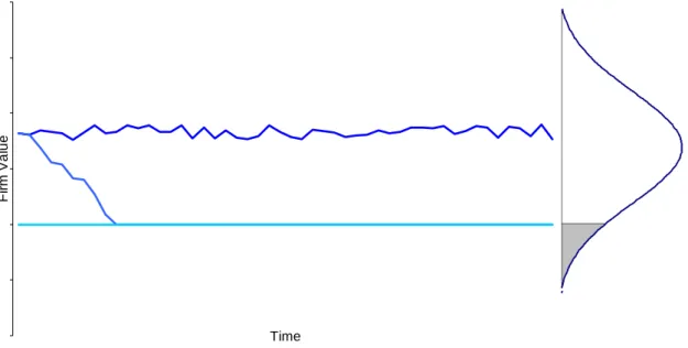
Figure 1. Default vs. no default
Time Fi rm V a lu e
Firm Value: No Default Firm Value: Default Debt Value = Asset Value = Default Barrier
The firm could face two different outcomes. First, there is no default and the value of the firm remains above the debt value. The equity value is the difference between the firm’s value and the debt value. Second, there is default and the value of the firm goes below the debt value, i.e. bondholders receive the remaining value of the firm and the equity holder receives the residual value, if there is any. The probability distribution of the firm’s value is shown to the right in Figure 1. The lower grey area describes the probability of default and the larger that area is, the larger the credit spread.
The logic behind the boundaries could also be illustrated with option pricing theory. The payoff from the equity holder to the bondholder could be replicated by a short put option on the firm value. The debt holder can receive the face value of debt, at most, but do not gain anything in excess of that. If the firm goes below the default point (grey line) the debt holder only receive a fraction
The Merton model
of the face value, i.e. the remaining value of the firm if there is no residuals value (see Figure 2).
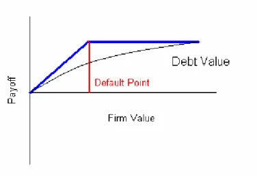
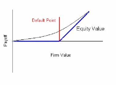
Figure 2. Short put on firm value
The equity holder only receives the upside of the debt value in contrast to the debt holder. In the event of default the equity holders are not expecting to receive anything unless the firm’s value is higher than the debt value. The equity holders are entitled to the residual value, i.e. the value above the debt value. In terms of option theory, this could be explained as a long position in a call option on the firm’s value owned by the equity holders (see Figure 3).
The Merton model
Figure 3. Call on firm value
This example of how the equity and debt could be explained by option theory is the groundwork in Merton’s model for valuing defaultable debt (see Appendix 1). It is also the link between equity and debt since they both could be expressed in relation to the firm value. This relationship has been known for a long time and the two markets are becoming more and more interlinked (Kassam, 2003). One of the easiest ways to verify this relationship is by examining the credit spreads and the implied equity volatility in the market. The two values have moved together for a long period, and it reveals that both markets discount the risk of the firm similarly. As an illustration, an example of
the credit spread for Ericsson and equity implied volatility11 is shown in Figure
4.
The Merton model
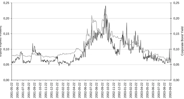
Figure 4. Implied volatility and the bond yield
0,00 0,05 0,10 0,15 0,20 0,25 2001 -0 5 -22 2001 -0 6 -22 2001 -0 7 -22 2001 -0 8 -22 2001 -0 9 -22 2001 -1 0 -22 2001 -1 1 -22 2001 -1 2 -22 2002 -0 1 -22 2002 -0 2 -22 2002 -0 3 -22 2002 -0 4 -22 2002 -0 5 -22 2002 -0 6 -22 2002 -0 7 -22 2002 -0 8 -22 2002 -0 9 -22 2002 -1 0 -22 2002 -1 1 -22 2002 -1 2 -22 2003 -0 1 -22 2003 -0 2 -22 2003 -0 3 -22 2003 -0 4 -22 2003 -0 5 -22 2003 -0 6 -22 2003 -0 7 -22 2003 -0 8 -22 2003 -0 9 -22 E q ui ty I m p li ed V o la ti li ty 0,00 0,05 0,10 0,15 0,20 0,25 C o rp o rat e B ond Y ie ld
Equity Implied Volatility (ATM Eric B) Corporate Bond Yield (LMETEL 6 3/8 06/06)
Figure 4 is intuitive: the greater the uncertainty in the market (higher implied volatility) the larger the discount factor is in the bond market (higher credit spread). Hence, the investors discount the prices similarly independent on whether it is in the equity market or in the bond market (Kassam, 2003). Valuable insights could be obtained by using both markets in the analysis, which is captured in our model.
Data
4
Data
Data was gathered in order to test the Merton model on ABB and Ericsson during different time periods. The criteria for choosing the time period were that the markets should not be stable and that the value of the bond and the equity should fluctuate. There should also be suitable outstanding bonds during the same time period for both companies. It allows us to draw conclusions based on different scenarios and examine the model in detail. In our case, the
time period was from 31st of December 2001 to June 28th 2003 and the data was
obtained on a daily basis. Daily data is important in a trading perspective, since trading can take place on any single day. Furthermore, the study is supposed to test the practical use of the Merton model and daily application is necessary to get reliable results. The sections below describe the data in detail divided into three different sections: Firm Data, Bond Data, and Market Data.
4.1
Firm Data
The individual firms were chosen based upon four requirements. First, the firm must have issued one outstanding bond with similar maturity that would be a good proxy for all debt. Second, changes in leverage over the time period are desirable to determine how the model works. Third, they should be among the largest firms on the Stockholm Stock Exchange (“A-listan, Mest Omsatta”). Fourth, a downgraded in the rating is desirable since that will imply that the company is facing a higher probability of default. The companies chosen are Ericsson and ABB, which fulfilled the requirements. Both companies have outstanding corporate bonds in Euros and stocks traded on the Stockholm Stock Exchange. The rating of the two companies have changed during the period of study, and was at the end of the period B1 (Moody’s) and BB (S&P) for
Ericsson and B1 (Moody’s) and BB- (S&P) for ABB (Bloomberg)12.
Data
The most important firm specific information needed was the capital structure. The capital structure is a major component in the Merton model and it was obtained from quarterly and annual reports (book values), which were available at the School of Economics library. More specifically, the balance sheet was examined and the focus was the debt and equity proportion.
4.2
Bond Data
The bond data is the information about the bond itself. There are several factors that are important for valuing the bond: time to maturity, coupon rate, face
value, annual or semiannual coupons. Indentures13 were also examined and
callable/putable and floating bonds were excluded, since the Merton model does not accurately incorporate them. The prices (in Euro) and the yield were also obtained and downloaded on a daily basis. The prices that were used were the end of the day mid-prices. The information was obtained from Bloomberg terminals and downloaded into Excel spreadsheets. The two bonds chosen
were: ABB Intl Finance ABB 5 1/8 01/11/06 and Ericsson LM Tel LMETEL 6
3/8 05/06. The bond issue for Ericsson is EUR 2,000 million and EUR 475 million for ABB.
4.3
Market Data
In addition to the firm data and the bond data, three complementary parameters were needed in order to use the Merton model. First, the risk-free interest rates are needed in order to discount the cash flows. The interest rates were extracted
from the zero-coupon yield curve (constructed by Nelson-Siegel14) and
downloaded from Nordea Analytics. Second, the exchange rates were needed in
13 Indenture is a written agreement between the issuer of a bond and his/her bondholders, usually specifying
interest rate, maturity date, convertibility, and other terms
14 Nelson-Siegel is an interpolation function to estimate the yield curve
Data
order to convert the capital structure into Euros, and were downloaded from DataStream. Third, the number of share outstanding and the share prices were downloaded from Bloomberg.
Model Implementation
5
Model Implementation
This section will discuss the adjustments we have done to the original Merton model and the data that has been applied. The data was not always in correspondence to the model, and had to be modified as described in this chapter.
5.1
Model Implementation
Merton’s model involves many assumptions and simplifications and some of them need to be changed to apply the model on market data. Merton made the assumption that the whole firms debt consist of one bond with no coupons. Equation 2 is Merton’s formula for valuation of debt assuming a zero-coupon bond.
( )
( )
⎭ ⎬ ⎫ ⎩ ⎨ ⎧ + = − 1 2 1 h N d h N Be D rτ (2) where B = face value D = value of debtThe expression within the brackets is the option feature in the valuation of the corporate bond. If the expression is equal to one the nominal value is discounted with the risk-free rate and considered risk-free. The option feature in this equation also contains the asset volatility, which is of interest to us in the analysis (see Appendix 2).
This equation is not applicable for our testing and therefore we used Merton’s
model for each coupon and the sum is the total value of the debt (see Appendix
Model Implementation - 20 -
( )
( )
∑
∑
= − = ⎭ ⎬ ⎫ ⎩ ⎨ ⎧ + = n i i n t t r t N h C d h N e c D t 1 1 2 1 τ (3) where tc = coupon size at time t (at maturity the face value is added to the coupon)
The reformulation of the model is not completely accurate since the default risk and therefore the probability of the coupons being paid out are dependent on each other, i.e. if one coupon defaults all the other also defaults. In the analysis it means that we would get a lower estimate of the risk than we otherwise would. However, the approach is not unique, and has been done before in research (for example Eom, et. al., 2002) and is a feasible approach of taking the coupons into consideration.
5.2
Firm Data
To estimate the fluctuations of the value of debt in the firms we assume that all debt could be replicated by one outstanding corporate bond. The assumption is made that the total value of the debt has the same volatility as the outstanding corporate bond and that the value will change as the bond price changes. However, some of the debt does not vary with the changes in prices of the corporate debt, such as pension liabilities (“provisions”), which we therefore held constant between the quarterly reports. The debt fluctuated on a day-to-day basis with the price changes of the outstanding corporate bond. Since we can obtain the market value of equity, the total value of the firms and its fluctuations over time can be identified. The procedure for estimating market value of assets is:
Equity Book -Provisions -Assets Total Debt Nominal t = t t t
Model Implementation t t t t Provisions 100 Bond of Price Market * Debt Nominal Debt ⎟+ ⎠ ⎞ ⎜ ⎝ ⎛ = t t
t Market Priceof Equity *Number ofShares
Equity = t t t Debt Equity Assets of Value Market = +
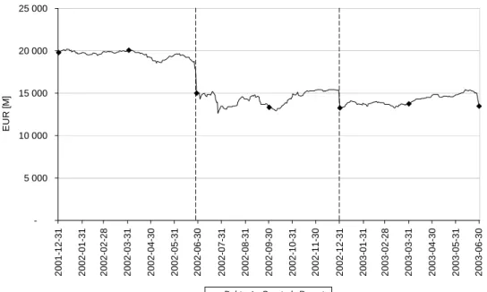
Figure 5 and 6 illustrates the estimated debt values for ABB and Ericsson, and the revised estimates at each quarterly report. The dots represent the quarterly reports when the total assets, current assets and provisions are adjusted. It is only at the quarterly reports that a balance sheet is published and when our estimations can be revised.
As can be seen in Figure 5 and 6 there are some errors in our estimates. For Ericsson at the end of June 2002, there is a large difference between our estimation and the value reported in the quarterly reports, i.e. there is a steep downward slope in Figure 5. The explanation why that occurs is that our proxy for the changes in the debt value (i.e. the bond) does not follow the actual changes accurately. Hence, the proxy provides occasional flaws in estimation. The flaws in estimation occur because of changes in (accounting) depreciation that the firm has decided to make. These errors are not possible to foresee since they are accounting issues and not market related. Hence, errors in our estimates will be present and cannot be avoided. When there are no changes in depreciation, there are no large errors in our estimates.
Model Implementation
Figure 5. Ericsson’s estimated debt value
-5 000 10 000 15 000 20 000 25 000 20 01-1 2 -3 1 20 02-0 1 -3 1 20 02-0 2 -2 8 20 02-0 3 -3 1 20 02-0 4 -3 0 20 02-0 5 -3 1 20 02-0 6 -3 0 20 02-0 7 -3 1 20 02-0 8 -3 1 20 02-0 9 -3 0 20 02-1 0 -3 1 20 02-1 1 -3 0 20 02-1 2 -3 1 20 03-0 1 -3 1 20 03-0 2 -2 8 20 03-0 3 -3 1 20 03-0 4 -3 0 20 03-0 5 -3 1 20 03-0 6 -3 0 EUR [ M ]
Debt Quarterly Reports
Figure 6. ABB’s estimated debt value
10000 15000 20000 25000 30000 35000 40000 2001- 12-31 2002- 01-31 20 02-28 2002- 03-31 2002- 04-30 2002- 05-31 2002- 06-30 2002- 07-31 2002- 08-31 2002- 09-30 2002- 10-31 2002- 11-30 2002- 12-31 2003- 01-31 2003- 02-28 20 03-31 2003- 04-30 2003- 05-31 2003- 06-30 E UR [ M ]
Debt Quarterly Reports
The equity prices that are downloaded from Bloomberg are adjusted for corporate actions, such as equity splits, which mean that the number of shares
Model Implementation
outstanding today can be used in conjunction with the historical prices from Bloomberg.
5.3
Bond data
From the bond indenture for Ericsson’s bond we discovered that the coupons size had changed three times since the bond was issued. This has to be taken into consideration; otherwise our estimation will differ from the market price. The occurrence of the change is due to a decrease in rating. The actual change happened the last day in May the year the coupon changed. One could argue that the market had already incorporated that the coupon would change before May since it is known that a decrease in rating will lead to an increase of yield by 25 basis points. But, since we do not know the day at which the market believes that the coupon will change, we used the last day in May since that is the day it actually happened. The ABB bond does not have this feature in its indenture.
The prices of the bonds downloaded from Bloomberg are clean prices. This means that we need to consider accrued interest in our model for the coupons. To adjust for this we argue that the companies continuously pay out coupons and repay their loans. The logic behind this is our assumption of letting the total value of the debt to be a proxy for the outstanding bond, i.e. because the companies have several bonds and loans. The bonds will payout fractions of coupons and face values and the loans will continuously be paid back. The coupon payment each day is a then a fraction (1/360) of the coupon size. The illustration in Figure 7 describes the process of finding the fractions of the next coupon:
Model Implementation
- 24 -
Figure 7. Coupon value
c1 c2
t1
τ t2
ttoday
If the time today is at tBtodayB the fraction of cB1B that we are entitle to is:
τ* cB1B
This means that at time tBtodayB we are entitling to:
τ* cB1B+ cB2+ cB B3B+…+cBn Bof the coupons.
5.4
Market data
In the original Merton model the yield curve is assumed to be flat, but to get an accurate analysis this has to be adjusted. We change the euro-government interest rates each day. They are obtained from the zero-coupon risk-free yield curve today, 1-year from today, 2-year from today etc, (from Nordea Analytics). They are interpolated to get the correct rates, i.e. the rate from today to the coupon payment as described below:
1 1) ( 365⎟⎠ − − + − ⎞ ⎜ ⎝ ⎛ t t t i i i τ (4) where 1 − t
i = zero coupon risk-free rate one year before from time t
t
i = zero coupon risk-free rate at time t
t T − =
Model Implementation
Huang and Huang (2003) argued that there is a liquidity premium. Therefore, an adjustment of 20 basis points is done, which is an estimation based on Huang and Huang’s conclusion. The new risk-free rate in Merton then becomes: t t l r i + = (5) where l = liquidity premium t
i = zero coupon risk free rate at time t
t
Test Procedure
6
Test Procedure
The first step in the test procedure is to gather data for the different companies. Thereafter, the data is applied in Merton’s model where we want to obtain the volatility of the firms’ assets. We insert the market price of the bond and the only unknown parameter in the model is then the asset volatility. This is achieved by iteration to obtain the volatility of the firms’ assets by minimizing the errors (setting the squared errors to zero) between the market price of the bond and the price from Merton’s model. The procedure is done in Excel where programming in Visual Basic (VBA) allowed for computations and iterations to be done automatically (see Appendix 3).
Once we have the asset volatility we argue that the extreme values that are observable in the market are fundamentally incorrect. Figure 8 and 9 illustrates the asset volatility (black line) and illustrates that there are extreme values present in the data. The risk in a company will not change radically from day to day. However, the risk can, of course, change during the life span of the company but not as drastically as the market implies. This argument is not
remarkable, but already discussed by Shiller (1981), that stated, “asset markets
[do not] in fact generate fundamental valuations. The speculative content of market prices is all too apparent in their excessive volatility”. As can be seen in Figure 8 and 9 the volatility of assets fluctuates significantly over time and there are several drastic changes. These changes are, as mentioned before, not necessarily accurate since the risk in the assets of firms does not drastically change on one trading day. Therefore, our approach is to smooth the volatility over time, which would allow the risk to change, but not as drastic as the market imply.
Test Procedure Figure 8. Ericsson’s estimated asset volatility
0,0 0,1 0,2 0,3 0,4 0,5 0,6 0,7 0,8 0,9 1,0 2 001- 12-3 1 2 002- 01-3 1 2 0 02-2 8 2 002- 03-3 1 2 002- 04-3 0 2 002- 05-3 1 2 002- 06-3 0 2 002- 07-3 1 2 002- 08-3 1 2 002- 09-3 0 2 002- 10-3 1 2 002- 11-3 0 2 002- 12-3 1 2 003- 01-3 1 2 003- 02-2 8 2 0 03-3 1 2 003- 04-3 0 2 003- 05-3 1 2 003- 06-3 0 As s e t Vo la tilit y
Asset Volatility MA 20 Exponential Smoothing MA 40
Figure 9. ABB’s estimated asset volatility
0,0 0,1 0,2 0,3 0,4 0,5 0,6 0,7 0,8 0,9 1,0 2 001- 12-3 1 2 002- 01-3 1 2 0 02-2 8 2 002- 03-3 1 2 002- 04-3 0 2 002- 05-3 1 2 002- 06-3 0 2 002- 07-3 1 2 002- 08-3 1 2 002- 09-3 0 2 002- 10-3 1 2 002- 11-3 0 2 002- 12-3 1 2 003- 01-3 1 2 003- 02-2 8 2 0 03-3 1 2 003- 04-3 0 2 003- 05-3 1 2 003- 06-3 0 As s e t Vo la tilit y
Asset Volatility MA 20 Exponential Smoothing MA 40
There are many different techniques for smoothing values over time (for example, moving average, exponential smoothing, and regressions). Moving average 20, 40, and an exponential smoothing are presented in Figure 8 and 9.
Test Procedure
We chose a moving average of 20 days (MA20) technique that is simplistic, but provides a smoothing of the volatility compared to the original curve. We argue that the smoothed curve from MA20 is a reasonable asset volatility without the overreactions that occur on some days. The discrepancies in the market are found when the model’s asset volatility diverges too much from the smoothed asset volatility.
In order to find the discrepancies we need to use Merton’s model again and insert the estimated (smoothed) asset volatility in the model to obtain a new bond price. In other words, all variables are unchanged except asset volatility, and a new bond price is estimated for each day. This is also done using Excel and programmed in Visual Basic. The new price is the price of the bond without overreactions that are present some days, which now could easily be compared with the market value of the bond. An indication whether the bond is under or overvalued could then be identified. The whole process of how the test procedure works is illustrated in Figure 10. The arrows illustrate the process flow and the boxes different data or operations.
Test Procedure
Figure 10. Diagram of test procedure
Input Data
Merton Model (iteration to find Asset Volatility)
Trading Strategies Estimated Asset
Volatility
Moving Average to find Estimated Asset Hedge Ratio Bond Price Merton Model Result: Strategy 1 Result: Strategy 2 Result: Strategy 3 Result: Strategy 4 Result: Strategy 5 Equity & Bond Price
Risk-free Rate Bond Indenture
Leverage
Framework for Trading Simulation
7
Framework for Trading Simulation
Before proceeding to the trading simulation the buy/sell indicator from the model had to be established and the hedge ratio that is necessary for two of the strategies has to be derived.
7.1
Implementation of Trading Simulation
This section will discuss the implementation of the trading simulation and the assumptions and restrictions imposed.
An indication of when the model would signal, “buy” or “sell” had to be determined, i.e. when the market value of the bond is too high in relation to the estimated model price and vice versa. The market bond prices and the estimated bond prices are plotted in Figure 11 and 12.
Figure 11. Ericsson - Market bond price and estimated bond price
65 70 75 80 85 90 95 100 105 110 115 2001-1 2 -3 1 2002-0 1 -3 1 2002-0 2 -2 8 2002-0 3 -3 1 2002-0 4 -3 0 2002-0 5 -3 1 2002-0 6 -3 0 2002-0 7 -3 1 2002-0 8 -3 1 2002-0 9 -3 0 2002-1 0 -3 1 2002-1 1 -3 0 2002-1 2 -3 1 2003-0 1 -3 1 2003-0 2 -2 8 2003-0 3 -3 1 2003-0 4 -3 0 2003-0 5 -3 1 2003-0 6 -3 0 Pri c e
Framework for Trading Simulation
- 32 -
Figure 12. ABB - Market bond price and estimated bond price
40 50 60 70 80 90 100 110 200 1-1 2 -3 1 200 2-0 1 -3 1 200 2-0 2 -2 8 200 2-0 3 -3 1 200 2-0 4 -3 0 200 2-0 5 -3 1 200 2-0 6 -3 0 200 2-0 7 -3 1 200 2-0 8 -3 1 200 2-0 9 -3 0 200 2-1 0 -3 1 200 2-1 1 -3 0 200 2-1 2 -3 1 200 3-0 1 -3 1 200 3-0 2 -2 8 200 3-0 3 -3 1 200 3-0 4 -3 0 200 3-0 5 -3 1 200 3-0 6 -3 0 Pr ic e
Estimated Bond Price Bond Price
The ratio is the relation between the two prices. The “signaling-points” should not be too narrow since it would then indicate an action (buy or sell) when the potential profit is rather small, and when the transaction costs would eliminate all potential profits. Given that the spread varies over time the signaling should be adjusted to fit the bid-ask spread. Hence, if there is a large bid-ask spread there needs to be a larger mispricing otherwise the trading costs would eliminate all potential profits. We are not including the bid-ask spread in our research, and therefore a static signaling point was assumed. We decided to only consider large errors and not try to trade on smaller mispricings, since it is more difficult to determine if smaller changes are profitable (when the bid-ask spread is not included). A difference between the market price and the new estimated price of 5% was considered a large error and therefore the boundaries are 1.05 and 0.95. The procedure is explained below:
Bond of Value Estimated Bond of Value Market Bond of Value Estimated Bond of Value Market f f1+0.05=1.05 ⇒
Framework for Trading Simulation
This result from the analysis means that the market value of the bond is overvalued and therefore “sell” is indicated. The position is kept until the market value of the bond is equal to the estimated value of the bond, or if a different indication is detected.
Bond of Value Estimated Bond of Value Market Bond of Value Estimated Bond of Value Market p p1−0.05=0.95 ⇒
When this result is indicated in the analysis, the market value of the bond is undervalued, and therefore the model indicates, “buy”. Again, the position is kept until the market value of the bond is equal to the estimated value of the bond, or if a different indication is detected. Figure 13 illustrates the ratio between the market price of the bond and the estimated bond price. The two horizontal lines in the graphs indicate when the models signals either buy or sell. For Ericsson there are 28 buy and 64 sell signals (7 periods) and for ABB there are 74 buy and 85 sell signals (11 periods). A period is characterized by a new indication (either buy or sell), but can consist of one signal or several adjacent signals.
Framework for Trading Simulation
Figure 13. ABB and Ericsson - Ratio between market bond price and estimated bond price 0,70 0,75 0,80 0,85 0,90 0,95 1,00 1,05 1,10 1,15 1,20 200 1-1 2 -3 1 200 2-0 1 -3 1 200 2-0 2 -2 8 200 2-0 3 -3 1 200 2-0 4 -3 0 200 2-0 5 -3 1 200 2-0 6 -3 0 200 2-0 7 -3 1 200 2-0 8 -3 1 200 2-0 9 -3 0 200 2-1 0 -3 1 200 2-1 1 -3 0 200 2-1 2 -3 1 200 3-0 1 -3 1 200 3-0 2 -2 8 200 3-0 3 -3 1 200 3-0 4 -3 0 200 3-0 5 -3 1 200 3-0 6 -3 0 ABB Ericsson Sell Buy
Since there is only one observation per day, the assumption is that the trade can be executed the same instance as the model indicates that a transaction should be made, i.e. when the (closing) price indicate “sell” the transaction is immediately executed. This is the most realistic assumption that we could make since in reality the trading is continuous, and the sell or buy signal could occur any second as long as the trading is open. Third, the evaluation of the different strategies were done using initial investment/portfolio of 1 (or 100%) and this initial portfolio was accumulated with the daily return, explicitly the value of the portfolio fluctuated daily with the performance of the different strategies. This approach was used since it allows us to compare the different strategies at any point during the time period and evaluating the strategies while they are still active and not only when they are finalized and a realized profit/loss has occurred. Borrowing money to increase the position was not allowed, since it would make the comparison more difficult.
Framework for Trading Simulation
There are some simplifications that have been made in the evaluation. The simplifications are not affecting the results substantially, and are excluded since they do not add value to the analysis. The first simplification is that the portfolio does not have any return (not even risk-free rate) when no security is held. The effect of that would be that the trading strategies that do not have a position for long periods would increase their performance compared to the strategies that are fully invested most of the time.
Another simplification is that the coupons and dividends are not reinvested or compounded at the risk-free rate. In other words, it is not “total return” that is of interest, but the return that can be generated by trading.
In the trading simulation, there are four possible positions to take in different combinations (see Appendix 4). They are; short bond, long bond, short equity, and long equity. The change in value of the position in relation to a change in asset volatility is shown in Table 1.
Table 1. Changes in value of a position when asset volatility increases
Position Value of position
Short Bond (Put on firm value) Increase
Long Equity (Call on firm value) Increase
Long Bond (Put on firm value) Decrease
Short Equity (Call on firm value) Decrease
If Asset Volatility Increases
The positions in Table 1 provide examples that will be used to test the model and provide insight to when it is useful. However, there are many other positions that can be taken, but the four above provide a good range of different trades. Other, more complex strategies could possibly provide additional profits/losses, but are outside the scope of this study.
Framework for Trading Simulation
- 36 -
7.2
Hedging
Two of the trading strategies will involve a hedge ratio, which is explained in this section. The hedge is set up by the link between equity and corporate bond, which implies that the value change of both equity and bonds could be expressed in relation to the change in firm value. The relationship can be derived from Merton’s work, and is explained and derived in Appendix 5. In brief, the hedge ratio is how many stocks you need to hold in order replicate the price change of one bond (see Appendix 6).
( )
( )
(
)
( )
( )
(
)
∑
∑
∑
∑
= = = = − = − = ∂ ∂ = ∂ ∂ ∂ ∂ n i i n i i i n i i i n i i h N h N h N C h N C E D V E V D 1 1 1 1 1 1 1 1 1 1 (6)The risk in equity is always higher than the risk in the bond, and therefore the hedge ratio is always less than one. A higher ratio indicates that the risk in equity and bond market is becoming more interlinked. As said before, when the leverage is higher the bond will behave more like equity. In Figure 14 the hedge ratios for both Ericsson and ABB are shown.
Framework for Trading Simulation Figure 14. Graph of hedge ratios - Ericsson and ABB
0,00 0,05 0,10 0,15 0,20 0,25 0,30 0,35 0,40 200 1-1 2 -3 1 200 2-0 1 -3 1 200 2-0 2 -2 8 200 2-0 3 -3 1 200 2-0 4 -3 0 200 2-0 5 -3 1 200 2-0 6 -3 0 200 2-0 7 -3 1 200 2-0 8 -3 1 200 2-0 9 -3 0 200 2-1 0 -3 1 200 2-1 1 -3 0 200 2-1 2 -3 1 200 3-0 1 -3 1 200 3-0 2 -2 8 200 3-0 3 -3 1 200 3-0 4 -3 0 200 3-0 5 -3 1 200 3-0 6 -3 0
Hedge Ratio ABB Hedge Ratio Ericsson
To verify that our hedge ratios were reasonable and that the two markets discount the risk similarly, i.e. that the prices move in tandem, the price changes were plotted. As can be seen in Figure 15 and 16 there is a linear relationship and on average the ratios are 0.0858 and 0.0523 over the whole period. A higher value for ABB than Ericsson is expected, since the hedge ratio shown in Figure 14 is higher for most of the period. The conclusion is that the hedge ratios are reasonable and a fundamental relationship between the two securities exists.
Framework for Trading Simulation Figure 15. ABB - Price changes in equity vs. bond
y = 0.0858x -8% -6% -4% -2% 0% 2% 4% 6% 8% -10% -8% -6% -4% -2% 0% 2% 4% 6% 8% 10%
Price change in Equity [%]
P ric e c h an ge i n B o n d [% ] ABB
Figure 16. Ericsson - Price changes in equity vs. bond
y = 0.0523x -8% -6% -4% -2% 0% 2% 4% 6% 8% -10% -8% -6% -4% -2% 0% 2% 4% 6% 8% 10%
Price change in Equity [%]
P ric e c h an ge i n B o n d [% ] Ericsson - 38 -
Trading Simulation
8
Trading Simulation
In order to test the model and the practical usefulness of it, five different trading strategies were developed and tested during the specified time period. The common argument for all of them is that they can be implemented by portfolio managers and provides information about the usefulness of the model. The equity, fixed income, and mixed fund do not isolate the asset volatility, i.e. is not delta hedged. Hence, there are several other factors that might be of more importance than the asset volatility to the value of the fund. Still, testing the strategies can provide insight of how, if at all, important the asset volatility is for funds of this type. The hedge funds are delta hedged, and therefore exposed solely to the asset volatility. Therefore, the strategy is most important when trying to establish if the Merton model is useful or not.
The different trading strategies were tested and evaluated against a benchmark. For the first strategy (the hedge fund approach), the benchmark is zero. The approach includes two offsetting positions, which results in no sensitivity to price changes, and therefore the return is expected to be zero. For two strategies (the mixed fund approach and fixed income approach) the benchmark is holding the bond, which is applicable since the risk and return in the portfolios are similar to holding the bond. For the last strategy (the equity fund approach) the benchmark is to hold the equity, which is most applicable when only the equity is traded. Then, a comparison could be made in terms of risk and return. The volatility was presented as the standard deviation (sigma). Additionally, a Sharpe-ratio was calculated that creates a ratio for comparing the different strategies in relation to their benchmark’s return and risk. The ratio is:
Trading Simulation - 40 - P B P R R Ratio Sharpe σ − = (7) where P
R = return on the portfolio
B
R = return on the benchmark
P
σ = standard deviation of portfolio
8.1
Time Period
The comparisons of the results are divided into three different periods. The
whole period is examined, which is the period from December 31P
st P 2001 to June 28P th P
2003. Then a division of the periods is done so that the comparisons can be made on semiannual basis (20011231-20020628, 20020628-20021231, and 20021231-20030630).
8.2
Ericsson - Bond and Equity
The bond had the largest price decrease in the first semiannual period, and it then improved its performance significantly. There is a u-shape in the bond returns that shows that the bond has clearly recovered and that the valuation is back to were it started at the beginning of the period.
When examining the equity, the most interesting conclusion that can be drawn from Figure 17 is that the equity had an extreme performance in all periods. The first two periods the equity value decreased significantly, while the third period had an increase.
8.3
ABB - Bond and Equity
The pattern for the bond, and equity in ABB, are similar to the results for Ericsson. The equity had a long decrease in value, while the bond presented the
Trading Simulation
same u-shaped pattern as the bond for Ericsson did. The similarity in return patterns is dependent on that both companies experienced crisis during this period.
Figure 17. Ericsson - Market bond price and equity price
40 50 60 70 80 90 100 2001 -1 2 -31 2002 -0 1 -31 2002 -0 2 -28 2002 -0 3 -31 2002 -0 4 -30 2002 -0 5 -31 2002 -0 6 -30 2002 -0 7 -31 2002 -0 8 -31 2002 -0 9 -30 2002 -1 0 -31 2002 -1 1 -30 2002 -1 2 -31 2003 -0 1 -31 2003 -0 2 -28 2003 -0 3 -31 2003 -0 4 -30 2003 -0 5 -31 2003 -0 6 -30 B ond P ri c e - 1 2 3 4 5 6 E qui ty P ri c e
Market Bond Price Equity Price
Figure 18. ABB - Market bond price and equity price
40 50 60 70 80 90 100 2001 -1 2 -31 2002 -0 1 -31 2002 -0 2 -28 2002 -0 3 -31 2002 -0 4 -30 2002 -0 5 -31 2002 -0 6 -30 2002 -0 7 -31 2002 -0 8 -31 2002 -0 9 -30 2002 -1 0 -31 2002 -1 1 -30 2002 -1 2 -31 2003 -0 1 -31 2003 -0 2 -28 2003 -0 3 -31 2003 -0 4 -30 2003 -0 5 -31 2003 -0 6 -30 B ond P ri c e 0 2 4 6 8 10 12 14 E qui ty P ri c e
Trading Simulation
Table 2. Bond return
Time Period 011231-020628 020628-021231 021231-030630 011231-030630 Ericsson Period Return -19.33% 6.17% 16.23% -0.45% ABB Period Return -10.99% -20.41% 31.29% -6.99% Bond Return
Table 3. Equity return
Time Period 011231-020628 020628-021231 021231-030630 011231-030630 Ericsson Period Return -75.03% -39.75% 40.50% -78.86% ABB Period Return -17.83% -69.67% 6.08% -73.57% Equity Return
8.4
Strategy 1: Hedge Fund Approach
The first strategy is the most active one, where the trading takes place as soon as the model signals “buy” or “sell”. The positions taken are long and short positions simultaneously in equities and bonds. The reasoning behind the strategy is that when the model indicates “buy” or “sell” a bet on that the market volatility is incorrect is taken. Hence, the relation of sigma is inversed between holding the bond and the equity, shorting one and holding the other creates a bet on volatility. However, at the same time a long-short position eliminates the credit risk since the long-short position will offset the changes in value between the two. This strategy is an alternative for portfolio managers that want to find discrepancies in the market, but that are not necessary interested in holding the bond for a longer time period.
Trading Simulation
Table 4. Illustration of the hedge fund approach
Indication from Merton model
Expected movement
of Asset Volatility Position Expected value
“Sell” Increase Short Bond and Long
Equity Increase
“Buy” Decrease Long Bond and Short
Equity Increase
No indication 0 No Position 0
8.4.1 Ericsson - Hedge Fund Approach
The hedge fund approach simulation resulted in several trades that were executed and held for a number of days. There were a total of 7 periods where there were indications of “buy” or “sell”. There are many trades that are necessary for this strategy since both the equity and bond is traded simultaneously. Hence, a total of 28 transactions had to be carried out (14 bond transactions and 14 equity transactions). The most significant characteristic of this approach is that there are long periods when no trading takes place (especially in the first and third period), which means that the fund has no position and no market risk exists (see Figure 19). Hence, regardless of what happens to the corporate bond and the equity, the fund will keep its value in absolute terms. The first period has a negative Sharpe-ratio and was the result of trading with negative return in the end of the period. The negative trades occur at the very end of the period, which prevents the fund from having a possibility to recover. The two other periods had positive Sharpe-ratios and the trades provided positive returns.
8.4.2 ABB - Hedge Fund Approach
There were 11 periods with buy and sell signals for the hedge fund, and resulted in a total of 44 trades (since transactions in both the equity and bond
Trading Simulation
are necessary each time). Again the hedge fund approach is very active and involves a lot of trading. However, there are long periods when no actual position is taken, and when the there is no return (see Figure 20). The best performance is achieved in the first two periods, while the last period has the negative return. Although, when considering the whole period the performance is positive.
Figure 19. Ericsson - Hedge fund approach
0,80 0,90 1,00 1,10 1,20 1,30 1,40 1,50 1,60 1,70 2001-1 2 -3 1 2002-0 1 -3 1 2002-0 2 -2 8 2002-0 3 -3 1 2002-0 4 -3 0 2002-0 5 -3 1 2002-0 6 -3 0 2002-0 7 -3 1 2002-0 8 -3 1 2002-0 9 -3 0 2002-1 0 -3 1 2002-1 1 -3 0 2002-1 2 -3 1 2003-0 1 -3 1 2003-0 2 -2 8 2003-0 3 -3 1 2003-0 4 -3 0 2003-0 5 -3 1 2003-0 6 -3 0 Re tu rn
Hedge Fund Buy / Sell Indication
Benchmark
Trading Simulation Figure 20. ABB – Hedge fund approach
0,80 0,90 1,00 1,10 1,20 1,30 1,40 1,50 1,60 1,70 2001- 12-31 2002- 01-31 20 02-28 2002- 03-31 2002- 04-30 2002- 05-31 2002- 06-30 2002- 07-31 2002- 08-31 2002- 09-30 2002- 10-31 2002- 11-30 2002- 12-31 2003- 01-31 2003- 02-28 20 03-31 2003- 04-30 2003- 05-31 2003- 06-30 Re tu rn
Hedge Fund Buy / Sell Indication
Benchmark
Table 5. Results – Hedge fund
Time Period 011231-020628 020628-021231 021231-030630 011231-030630
Ericsson
Period Return -5.62% 15.20% 2.11% 11.03%
Benchmark Return 0.00% 0.00% 0.00% 0.00%
Yearly Sharpe Ratio -1.54 1.45 1.11
-ABB
Period Return 11.20% 24.86% -7.44% 28.52%
Benchmark Return 0.00% 0.00% 0.00% 0.00%
Yearly Sharpe Ratio 1.60 0.78 -1.43
-Hedge Fund
8.5
Strategy 2: Mixed Fund Approach
The second strategy is to hold the bond as long as it is priced correct or too low, i.e. when the market volatility is above the “sell” indication. If the indication becomes “sell” the strategy changes to not having a position in the bond, and instead enters a position in the equity. Hence, the position in the equity will increase as the volatility increases and the portfolio will increase in value as sigma increase. Only holding the bond would have resulted in a decrease in
value, ceteris paribus. This strategy is attractive for the portfolio managers that
Trading Simulation
benefit from the specific characteristics of each market. The risk involved in this strategy is higher than for the hedge fund, since positions are taken and not hedged.
Table 6. Illustration of the mixed fund approach
Indication from Merton model
Expected movement
of Asset Volatility Position Expected value
“Sell” Increase Long Equity Increase
“Buy” Decrease Long Bond Increase
No indication - Long Bond
-8.5.1 Ericsson - Mixed Fund Approach
The mixed fund approach resulted in less trades than the hedge fund approach, since the indication “sell” only appeared in five different periods and the strategy then is to sell the bond and buy the equity. This resulted in a total of 10 transactions during the whole period since we need to buy or sell both equity and the bond. As can be seen in Figure 21, this approach follows the performance of the bond very well. There are a few trades, but they do not improve the results significantly. Also, the low Sharpe-ratios support that argument.
8.5.2 ABB - Mixed Fund Approach
The mixed fund actually performed worse than the bond itself, and had a negative Sharpe-ratio for two periods. As can be seen in Figure 22 the trading results for this strategy is rather poor with negative Sharpe-ratios and better performance by the benchmark. Also, there are five periods were there are sell signals. It means that the fund will change its exposure from bond to equity five times, which involves 10 equity transactions and 10 bond transactions.
Trading Simulation
Figure 21. Ericsson - Mixed fund approach
0,60 0,70 0,80 0,90 1,00 1,10 1,20 1,30 1,40 2001- 12-31 2002- 01-31 20 02-28 2002- 03-31 2002- 04-30 2002- 05-31 2002- 06-30 2002- 07-31 2002- 08-31 2002- 09-30 2002- 10-31 2002- 11-30 2002- 12-31 2003- 01-31 2003- 02-28 20 03-31 2003- 04-30 2003- 05-31 2003- 06-30 Re tu rn
Bond Return Mixed Fund Buy / Sell Indication
Figure 22. ABB – Mixed fund approach
0,20 0,40 0,60 0,80 1,00 1,20 1,40 2001- 12-31 2002- 01-31 20 02-28 2002- 03-31 2002- 04-30 2002- 05-31 2002- 06-30 2002- 07-31 2002- 08-31 2002- 09-30 2002- 10-31 2002- 11-30 2002- 12-31 2003- 01-31 2003- 02-28 20 03-31 2003- 04-30 2003- 05-31 2003- 06-30 Re tu rn
Trading Simulation Table 7. Results – Mixed fund
Time Period 011231-020628 020628-021231 021231-030630 011231-030630
Ericsson
Period Return -19.33% 13.09% 16.23% 6.03%
Benchmark Return (Bond) -19.33% 6.17% 16.23% -0.45%
Yearly Sharpe Ratio 0.00 0.50 0.00
-ABB
Period Return -9.14% -23.59% 21.15% -15.89%
Benchmark Return (Bond) -10.99% -20.41% 31.29% -6.88%
Yearly Sharpe Ratio 0.13 -0.06 -0.98
-Mixed Fund
8.6
Strategy 3: Fixed Income Fund Approach
An alternative approach is to hold the bond as long as it is valued fair or undervalued, but sell it as soon as the model indicates that it is overvalued. The objective of the fund is to hold bonds. The portfolio is rather simple since it consists of the bond or of nothing at all. It is the typical trading of a portfolio consisting of only bonds, no equities or other instruments.
Table 8. Illustration of the fixed income fund approach
Indication from Merton model
Expected movement of
Asset Volatility Position Expected value
“Sell” Increase No Position 0
“Buy” Decrease Long Bond Increase
No indication - Long Bond
-8.6.1 Ericsson - Fixed Income Fund Approach
The fixed income approach is the strategy that is most comparable to only holding the bond. However, the risk is somewhat lower since there are actually time periods when there are no positions at all. For three different periods the model gives indication of selling the bond, which means that we need to make 6 different transactions with the bond. Higher return of the fund in comparison
Trading Simulation
to the bond occurs since the fund manages to block some of the large decreases in price that occurs, more specifically in period two (see Figure 23). The result is very similar to the result for the mixed fund.
8.6.2 ABB - Fixed Income Fund Approach
The fixed income fund presented similar results as the mixed fund: the fund did not outperform the benchmark. As can be seen in Figure 24, there are five periods when a sell indication occurs, that results in selling and then buying back the bond five times (10 transactions).
Figure 23. Ericsson - Fixed income fund approach
0,60 0,70 0,80 0,90 1,00 1,10 1,20 1,30 1,40 2001- 12-31 2002- 01-31 20 02-28 2002- 03-31 2002- 04-30 2002- 05-31 2002- 06-30 2002- 07-31 2002- 08-31 2002- 09-30 2002- 10-31 2002- 11-30 2002- 12-31 2003- 01-31 2003- 02-28 20 03-31 2003- 04-30 2003- 05-31 2003- 06-30 Re tu rn
Trading Simulation
Figure 24. ABB – Fixed income fund approach
0,20 0,40 0,60 0,80 1,00 1,20 1,40 2001 -1 2 -31 2002 -0 1 -31 2002 -0 2 -28 2002 -0 3 -31 2002 -0 4 -30 2002 -0 5 -31 2002 -0 6 -30 2002 -0 7 -31 2002 -0 8 -31 2002 -0 9 -30 2002 -1 0 -31 2002 -1 1 -30 2002 -1 2 -31 2003 -0 1 -31 2003 -0 2 -28 2003 -0 3 -31 2003 -0 4 -30 2003 -0 5 -31 2003 -0 6 -30 Re tu rn
Bond Return Fixed Income Fund Buy / Sell Indication
Table 9. Results – Fixed income fund
Time Period 011231-020628 020628-021231 021231-030630 011231-030630
Ericsson
Period Return -19.33% 18.98% 16.23% 11.56%
Benchmark Return (Bond) -19.33% 6.17% 16.23% -0.45%
Yearly Sharpe Ratio 0.00 0.97 0.00
-ABB
Period Return -9.30% -22.43% 33.52% -6.06%
Benchmark Return (Bond) -10.99% -20.41% 31.29% -6.88%
Yearly Sharpe Ratio 0.12 -0.04 0.26
-Fixed Income Fund
8.7
Strategy 4: Equity Fund Approach
This strategy is to only trade the equity, and ignores the bond. This is an alternative that shows if the volatility in assets is useful for equity funds. This is an additional dimension to the portfolio management approaches that has been described above.
Trading Simulation Table 10. Illustration of the equity fund approach
Indication from Merton model
Expected movement
of Asset Volatility Position Expected value
“Sell” Increase Long Equity Increase
“Buy” 0 No Position 0
No indication - Long Equity
-8.7.1 Ericsson - Equity Fund Approach
The equity fund approach has a very low average annual return. However, it is important to realize that the time period is one of the worst in Ericsson’s history with poor stock performance. Considering the relative performance, the strategy had higher return than the benchmark. This strategy involves only trading with equity and a transaction is made when the model indicate a buy signal of the bond. The model signals a total of four periods of buy and it results in eight transactions of buying and selling equity. It is noteworthy that the return of the fund is extremely low for the first two periods, while the return for the last period is extremely high. The same performance characteristics were displayed for the equity itself. The performance of the fund for the whole periods is approximately 2 percent better than the benchmark.
8.7.2 ABB - Equity Fund Approach
The equity fund performed better than holding the bond and improved the trading results. The fund managed to withstand a few decreases, and therefore outperformed the benchmark (see Figure 26). However, in the first period the return of the fund was much lower than the benchmark. There are 6 buy indications that resulting in the fund withdrawing its equity position, and holding no position. There are 12 transactions in the equity market.