Graph Powers: Hardness Results, Good Characterizations and Efficient Algorithms. Dissertation

(1)

Hardness Results,

Good Characterizations and

Efficient Algorithms

Dissertation

zur

Erlangung des akademischen Grades

Doktor-Ingenieur (Dr.-Ing.)

der Fakult¨at f¨

ur Informatik und Elektrotechnik

der Universit¨at Rostock

Vorgelegt von

MSc. Ngoc Tuy Nguyen

Rostock, November 2009

(2)

Universit¨at Rostock. Institut fu¨r Informatik

Gutachter: Prof. Dr. Egon Wanke

Heinrich- Heine- Universit¨at D¨usseldorf. Institut fu¨r Informatik

Gutachter: Prof. Dr. Ekkehard K¨ohler

Brandenburgische Technische Universit¨at Cottbus. Institut fu¨r Mathematik

Tag der ¨offentlichen Verteidigung: 30. Oktober 2009

(3)

Abstract

Given a graphH= (VH, EH) and a positive integer k, the k-th power ofH, written

Hk_{, is the graph obtained from} _H _{by adding new edges between any pair of vertices}

at distance at most k inH; formally,Hk _{= (V}

H,{xy |1≤dH(x, y)≤k}).

A graph Gis the k-th power of a graph H if G=Hk_{, and in this case,} _H _{is a} _k_-th

root of G. For the cases of k = 2 and k = 3, we say that H2 _and _H3 _{is the} _square_, respectively, the cube of H and H is a square root of G =H2_{, respectively, a} _cube

root of G=H3_.

In this thesis we study the computational complexity for recognizing k-th pow-ers of general graphs as well as restricted graphs. This work provides new NP-completeness results, good characterizations and efficient algorithms for graph pow-ers. The main results are the following.

• There exist reductions proving the NP-completeness for recognizingk-th pow-ers of general graphs for fixed k ≥ 2, recognizing k-th powers of bipartite graphs for fixedk ≥3, recognizing k-th powers of chordal graphs, and finding k-th roots of chordal graphs for all fixed k ≥2.

• The girth of G, girth(G), is the smallest length of a cycle in G,

– For all fixed k ≥ 2, recognizing of k-th powers of graphs with girth at most 2⌊k

2⌋+ 2 is NP-complete.

– There is a polynomial time algorithm to recognize if G = H2 _{for some} graph H of girth at least 6. This algorithm also constructs a square root of girth at least 6 if one exists.

– There exists a good characterization of squares of a graph having girth at least 7. This characterization not only leads to a simple algorithm to compute a square root of girth at least 7 but also shows such a square root, if it exists, is unique up to isomorphism.

– There is a good characterization of cubes of a graph having girth at least 10 that gives a recognition algorithm in time O(nm2_{) for such graphs.} Moreover, this algorithm constructs a cube root of girth at least 10 if it exists.

(4)

recognition problem in terms of girth of the square roots.

• There is a good characterization of squares of strongly chordal split graphs that gives a recognition algorithm in time O(min{n2_{, m}_log_n_}_{) for such squares.} Moreover, this algorithm also constructs a strongly chordal split graph square root if it exists.

• There exists a good characterization and a linear-time recognition algorithm for squares of block graphs. This algorithm also constructs a block graph square root if one exists. Moreover, block graph square roots in which every endblock is an edge are unique up to isomorphism.

The almost results in thesis have been published in the following papers of journal and proceedings of conferences.

• “Computing Graph Roots Without Short Cycles”, Proceedings of the26th

In-ternational Symposium on Theoretical Aspects of Computer Science(STACS 2009), pp. 397 - 408.

Co-authors: Babak Farzad (Brock University, Canada), Lap Chi Lau (The Chinese University of Hong Kong), Van Bang Le (University of Rostock).

• “Hardness Results and Efficient Algorithms for Graph Powers”, to appear in:

Proceedings of the35th _{International Workshop on Graph-Theoretic Concepts}

in Computer Science(WG 2009).

Co-author: Van Bang Le (University of Rostock).

• “The square of a block graph”, to appear in: Discrete Mathematics (2009), doi:10.1016/j.disc.2009.09.004.

Co-author: Van Bang Le (University of Rostock).

(5)

Acknowledgments

Although a few words do not do justice to their contribution I would like to thank the following people for making this work possible.

First of all I would like to express my sincere gratitude to my advisor Professor Van Bang Le, for his patience, invaluable advice and encouragement throughout. His lectures and advices have been of great value for my research. This work would not have been possible without his support, patience and encouragement.

I wish to express my sincere thanks to Professor Andreas Brandst¨adt for a lot of personal help during the time. I thank Professor Egon Wanke and Professor Ekkehard K¨ohler for their reading and commenting on my thesis.

I am grateful to my co-authors for the joint works and successful discussions, and for allowing me to include the results in this thesis.

I am also grateful to colleagues of the Institute of theoretical informatics for their help and support during my study. Special thanks go to Roswitha Fengler, Katrin Erdmann, Christian Hundt and Ragnar Nevries for a lot of help.

Furthermore, I also would like to express my gratitude to my university, HongDuc, who recommended and encouraged me to study well. Especially, I am truly deeply grateful to all my colleagues at the Department of Computer Science, HongDuc University for their encouragements.

While working on this thesis, financial support by the Ministry of Education and Training, Vietnam (322 Project) by Grant No.3766/QD-BGD&DT is gratefully acknowledged. I am also grateful to DAAD for their support for me in learning German.

Great thanks go to my buddies for their support and encouragement. I also want to thank to all friends in Rostock - ”Rostockers” for everything we shared together over the years of living.

Last but not least, I am indebted to my parents, my sisters and brothers who have given me the best opportunities. All my love and thanks go to my wife Ha.nh and my children Qu`ynh Anh and Minh Lˆo.c. Without their love and gentle encouragement I could not complete this work. Thank you very much!

Rostock, November 4, 2009 Nguyˆe˜_{n Ngo.c T´uy}

(6)

List of Figures

3.1 Tail inH (left) and in G=H2 _(right) _{. . . 16}

3.2 Tail ink-th root H of Gand in G . . . 16

4.1 The graph G for the example instance of set splitting and k = 4 . 20 4.2 The bipartite 4-th root graph H of Gto the solution S1, S2 . . . 21

4.3 A bipartitek-th root H in Lemma 4.1.1 to the example solutionS1, S2 22 4.4 The graph G for the example instance of set splitting and k = 3 . 28 4.5 Cube root graph H to the solution S1,S2. . . 29

4.6 A chordal k-th root H in Lemma 4.2.1 to the example solution S1, S2 31 4.7 The chordal graphGfor the example instance of set splittingand k = 4 . . . 37

4.8 Fourth root graphH to the solution S1, S2 . . . 38

4.9 A k-th root H in Lemma 4.3.3 to the example solution S1, S2 . . . 41

5.1 The graph G for the example instance of set splitting _{. . . 45}

5.2 An example of rootH with girth 4 . . . 46

5.3 The graph G for the example instance of set splitting and k = 4 . 50 5.4 The fourth root graph H with girth six of Gto the solution S1, S2 . . 51

5.5 The graph G for the example instance of set splitting and k = 5 . 52 5.6 The fifth root graphH with girth six of Gto the solution S1, S2 . . . 53

5.7 A k-th root H with girth k+ 2 for even k in Lemma 5.2.1 . . . 54

5.8 A k-th root H with girth k+ 1 for odd k in Lemma 5.2.1 . . . 55

6.1 An input graph G(a), the subgraph F of G(b) and a square root H (c) constructed according to the proof of Theorem 6.2.4 . . . 66

(10)

NG(b); a (C3, C5)-free square root H (b) constructed by Algorithm

6.3.1: c3c5-free . . . 71 8.1 The vertices u, v are maximal vertices in the given graph . . . 84 8.2 An input graph G (a), a clique C in G (b) and a square root H (c)

constructed by Algorithm 8.1 . . . 87 9.1 Two block graphs (a) and (b) with the same square (c) . . . 94 9.2 An input graph G(a), the subgraph F of G(b) and a square root H

(c) constructed by Algorithm 9.3: BlockGraphRoot . . . 96

(11)

Part I

Introduction

(12)

Chapter 1 Overview

1.1 Introduction

In graph theory, graph H is a root of graph G = (V, E) if there exists a positive integerk such that xand y are adjacent inG if and only if their distance inH is at most k. If H is a k-th root of G, then we write G=Hk _{and call} _G_the _{k-th power}

of H. Graph powers and roots are fundamental graph-theoretic concepts and have been extensively studied in the literature, both in theoretic and algorithmic senses; see e.g., [17, 29, 42, 45, 46, 49] for recent results and the numerous references listed there.

The first motivation comes directly from the fact that root and root comput-ing are concepts familiar to most branches of mathematics. Any result on graph roots and powers would be a very valuable contribution in studying graph theory. Graph powers are also very useful in designing efficient algorithms for certain com-binatorial optimization problems. For instance, the papers [2, 1] used a (in linear time constructible) Hamiltonian cycle in the cube T3 _{of the nontrivial tree} _T _in their approximation algorithm for the Traveling Salesman Problem (TSP) with a parameterized triangle inequality. For the same problem, the approximation pro-posed in [9] used a Hamiltonian cycle in the square G2 _{of a 2-connected graph} _G. Note that these graph power-based algorithms are the best known approximations for this variant of theTSP problem. Note also that the square of any 2-connected graph is Hamiltonian is a fundamental and deep theorem in graph theory due to Fleischner [30], and the PhD thesis [44] provided an algorithm that constructs a Hamiltonian cycle in such a square in polynomial time.

Moreover, graph roots and powers are of great interest and have a number of possible applications in different disciplines. For example, in distributed computing (cf. [55, 51]), thek-th power of a graphGrepresents the possible flow of information duringk rounds of communication of a distributed network of processors organized according toG.

(13)

In radio frequency planning, certain situations are closely related to the coloring of the power of the associated radio network; in such applications, the associated radio network is the graph where vertices represent the transmitters and adjacencies between vertices indicate possible interferences. To avoid interference, transmitters which are close (at distance at most k in the graph) receive different frequencies. This problem is exactly the coloring problem onk-th powers of the graph. There are many studies on this problem. For example (cf. [8, 10, 21, 22, 69]), radio frequency planning without direct and hidden collisions in the radio networkG(also known as L(1,1)-labeling problem or distance-2 coloring problem) is equivalent to the coloring of the square G2 _of _{G, and has been well-studied.}

In computational biology, graph powers and roots, in particular tree powers and roots, are useful in the reconstruction of phylogeny (cf. [20, 50, 57, 15]).

Graph powers and roots are fundamental graph-theoretic concepts and have been extensively studied in literature, both in theoretic and algorithmic senses. These investigations considered both characterization and recognition problems, see [13, Sec. 10.6] for a survey and [46, 45] for the most recent papers.

For the characterization problem, in 1960, Ross and Harary [63], first studied the concept of a square of graphs. They characterized squares of trees and showed that tree square roots, when they exist, are unique up to isomorphism. Next, in 1967, Mukhopadhyay [56] provided a characterization of general graphs which have a square root. In 1974, Escalanteet al. [27] characterized graphs and digraphs with a k-th root. However, these characterizations are not good in the sense that they do not lead to a polynomial time recognition algorithms for such as graphs. In fact, such a good characterization may not exist as Motwani and Sudan proved that it is NP-complete to determine if a given graph has a square root [55].

The computational complexity of recognizing ofk-th powers of graphs was unre-solved until 1994 when Motwani and Sudan [55] proved that recognizing of square of graphs is NP-complete. Very recently, in 2006, Lau [45] proved the NP-completeness for recognizing of cubes of graphs. He conjectured that recognizing k-th powers of some graph is NP-complete for all fixed k ≥ 2 (cf. Conjecture 2.2.1, p. 11) and recognizing k-th powers of bipartite graphs is NP-complete for all fixed k ≥ 3 (cf. Conjecture 2.2.2, p. 12).

By the above-mentioned negative results of Motwani and Sudan, and of Lau, a natural way (in theory and in applications) in considering k-th powers of graphs is to restrict the root graphsH.

In this thesis, we study the computational complexity for recognizingk-th powers of general graphs as well as restricted graphs. In particular, the aim of this work is as follows.

• Reductions proving the NP-completeness for recognizingk-th powers of general graphs for fixed k ≥ 2, recognizing k-th powers of bipartite graphs for fixed

(14)

k≥3, recognizingk-th powers of chordal graphs, findingk-th roots of chordal graphs for all fixedk≥2, and recognizing k-th powers of graphs with girth at most 2⌊k

2⌋+ 2 for all fixed k≥2.

• Good characterizations of squares of a graph having girth at least seven and cubes of a graph having girth at least ten. Squares of graphs with girth at least six can be recognized in polynomial time.

• Good characterization of squares of strongly chordal split graphs that leads to a recognition algorithm in timeO(min{n2_{, m}_log_n_}_{) for such squares.}

• Good characterization and a linear-time recognition algorithm for squares of block graphs.

1.2 Contributions of the thesis

There are three parts in this thesis. In Part I after a brief introduction of motivations and overview of thesis (Chapter 1), Chapter 2 provides basic notion and facts used throughout the thesis.

The main results of this thesis appear in Part II and Part III.

Part II includes the NP-completeness results for recognizing k-th powers of graphs. Chapter 3 recalls the NP-completeness results on graph power recogni-tion problems in the literature. This chapter presents also some tools that are used in reductions in Chapter 4 and Chapter 5. Chapter 4 gives reductions proving the Conjecture 2.2.1 and Conjecture 2.2.2 are indeed true. This chapter also shows that recognizingk-th powers of chordal graphs andk-th roots of chordal graphs are NP-complete for all fixedk≥2. Chapter 5 considers the complexity for recognizingk-th powers of graphs with girth conditions. It shows that recognizing ofk-th powers of graphs with girth at most 2⌊k

2⌋+ 2 is NP-complete.

Part III includes four chapters presenting efficient algorithms for recognizing squares and cubes of some restricted graphs. Chapter 6 provides a good charac-terization for graphs that are squares of some graph of girth at least seven. This characterization not only leads to a simple algorithm to compute a square root of girth at least 7 but also shows that such a square root, if it exists, is unique up to iso-morphism. This chapter also shows that squares of graphs with girth at least six can be recognized in polynomial time. Chapter 7 gives a good characterization of graphs that are cubes of a graph having girth at least 10. This characterization leads to the immediate consequence that recognizing cubes of (C4, C6, C8)-free bipartite graphs is polynomial time, whereas recognizing cubes of general bipartite is NP-complete. Chapter 8 shows that there exists a good characterization of squares of strongly chordal split graphs that gives a recognition algorithm in time O(min{n2_{, m}_log_n_}₎

(15)

for such squares. Part III is closed by Chapter 9. This chapter provides good char-acterizations for squares of block graphs and a linear-time recognition algorithm for such squares. This algorithm also constructs a square block graph root if one exists. Moreover, block graph square roots in which every endblock is an edge are unique up to isomorphism.

(16)

Chapter 2 Background

Section 2.1 provides basic notions and definitions which are necessary for under-standing the remaining part of this thesis. In Section 2.2 we recall two fundamental problems on graph powers, and collect several facts that are related to this work.

2.1 Definitions and notation

Notions and definitions not given here can be found in any standard textbook on graph theory or graph algorithms, e.g. [11, 13, 68, 33, 35].

In the following we always consider finite, undirected and simple graphs G = (V, E) whereV is the vertex set ofGand E the edge set ofG. To avoid ambiguities we sometimes use V(G) or VG to refer to V and E(G) or EG to refer to E. The

cardinality of the vertex setV is denoted byn, and the cardinality of the edge setE is denoted by m. A set of graphs is generally called a graph class. Thecomplement

G of a graph G is the graph with vertex set VG defined by uv ∈ EG if and only

if uv 6∈ EG. A graph H = (VH, EH) is a subgraph of G = (V, E) if VH ⊆ V and

EH ⊆ E. A graph H = (VH, EH) is an induced subgraph of G, if it is a subgraph

of G and it contains all the edges uv such that u, v ∈ VH and uv ∈ EG. We say

that H is induced by VH and write G[VH] for H. Given a set of vertices X ⊆V, if

X = {a, b, c, . . .}, we write G[a, b, c, . . .] for G[X]. Also, we often identify a subset of vertices with the subgraph induced by that subset, and vice versa.

Let F denote a set of graphs. A graph G is F −f ree if none of its induced subgraphs is isomorphic to a graph in F.

Gisconnected if for allu, v ∈V,u6=v, there is a pathu, v-path inGconnecting u and v; otherwise, G is disconnected. A maximal connected subgraph of G is a subgraph that is connected and is not contained in any other connected subgraph.

The connected components of a graph are its maximal connected subgraphs.

LetG= (V, E) be a connected graph. A subset S⊂V is a cutset (or separator)

(17)

ofG ifG[V \S] is disconnected. For a positive integer k, ak-connected component

in a graph G is a maximal (induced) k-connected subgraph of G; the 1-connected components ofG are the usual connected components, and the 2-connected compo-nents ofGare also calledblocksofG. Ak-cutin a graph is a cutset withk vertices; a 1-cut is also called a cut-vertex. An endblock in a graph is a block that contains at most one cut-vertex of the graph.

An isomorphism from G to H is a bijection f : VG → VH such that uv ∈ EG if

and only iff(u)f(v)∈EH for all u, v ∈VG. We say “Gis isomorphic to H”.

IfGhas au, v-path, then thedistance fromutov, writtendG(u, v) is the length,

i.e., number of edges, of a shortest path in Gbetween u and v. Thediameter of G, writtendiam(G), is the maximum distance between two vertices (and∞if Gis not connected).

Fork≥1, letPk denote a chordless path withk vertices andk−1 edges, and for

k≥3, letCk denote a chordless cycle withk vertices andkedges. The length of the

cycle is the number k of its edges. An even (odd) path (cycle) is a path (cycle) of even (odd) length. Chordless cycles Ck, k ≥ 5, are holes. Chordless cycles C2k+1,

k ≥ 2, are odd holes. Complements Ck of chordless cycles Ck, k ≥ 5 are antiholes.

ComplementsC2k+1 of odd holes C2k+1, are odd antiholes.

Let G = (VG, EG) be a graph. We often write xy ∈ EG for {x, y} ∈ EG. We

sometimes also write x↔ y for the adjacency of x and y in the graph in question; this is particularly the case when we describe reductions in NP-completeness proofs. For disjoint sets of vertices X and Y, we write X ↔Y, meaning each vertex in X is adjacent to each vertex inY; if X ={x}, we simply write x↔Y.

The girth ofG, girth(G), is the smallest length of a cycle inG; in case G has no cycles, we set girth(G) =∞. In other words,Ghas girthkif and only ifGcontains a cycle of lengthk but does not contain any (induced) cycle of lengthℓ= 3, . . . , k−1. It is quite usual to measure the sparseness of a graph in terms of its girth; a graph is “sparse” if its girth is “large enough”. A girth(G) =∞ if and only ifG is a tree.

Note that the girth of a graph can be computed in timeO(nm) [41].

Definition 2.1.1 (Powers of Graphs)

Let H = (VH, EH) be a graph. Given a positive integer k, the k-th power of H,

written Hk_{, is the graph obtained from} _H _{by adding new edges between any pair of}

vertices at distance at mostk in H; formally, Hk_{= (V}

H,{xy |1≤dH(x, y)≤k}).

A graphG is the k-th power of a graph H if G=Hk_{, and in this case,} _H _{is a} _k-th

root of G.

For the cases of k = 2 and k = 3, we say that H2 _and _H3 _{is the} _square_,

respec-tively, the cube of H and H is a square root of G= H2_{, respectively, a} _{cube root}

(18)

Definition 2.1.2 (Neighborhood)

Let G= (V, E) be a graph and v ∈V.

• N(v) = {u|u∈V, u=6 v and uv∈E} denotes the (open) neighborhood of v,

• N[v] =N(v)∪ {v} denotes the closed neighborhood of v,

• Nk_{(v) =} _{_u_|_u_∈_V _and _{d(u, v) =}_k_} _{denotes the} _k_{-th neighborhood of} _v_,

Definition 2.1.3 (Degree of Vertex)

Let G= (V, E)be a graph and v ∈V. Set degG(v) =|NG(v)|, the degree of v in

G. The maximum degree is denoted ∆(G), minimum degree is denoted δ(G). A

vertex with degree 0 is called an isolated vertex. We call vertices of degree one in G end-vertices of G. A center vertex (or universal vertex) of G is one that is adjacent to all other vertices.

Definition 2.1.4 (Clique and Stable Set)

Let G = (V, E) be a graph. A set of vertices Q ⊆ V is called a clique in G if every two distinct vertices in Q are adjacent; A stable set or an independent set is a set of pairwise non-adjacent vertices.

Amaximal clique (stable set)is a clique (stable set) that is not properly contained in another clique(stable set).

A clique (stable set) is maximum if its cardinality is the maximum possible size of a clique (stable set) in G.

The clique number of graph, written ω(G), is the maximum clique size in G. The independence number of graph, written α(G), is the maximum independent set size inG.

The chromatic numberof graph, written χ(G), is the minimum number of colors needed to label the vertices so that adjacent veritices receive different colors.

The clique cover number of graph, written θ(G), is the minimum number of cliques in G needed to cover VG.

The next definitions give some special graph classes that we need in later chapters.

Definition 2.1.5 (Intersection Graph)

For a given setM of objects (for which intersection makes sense), the intersection graphGM of these objects has M as vertex set, and two objects are adjacent in GM

(19)

Definition 2.1.6 (Some Special Graph Classes)

• A complete graph is one in which every two distinct vertices are adjacent; a complete graph onk vertices is also denoted by Kk.

• A star is a graph with at least two vertices that has a center vertex and the

other vertices are pairwise non-adjacent. Note that a star contains at least one edge and at least one center vertex; the center vertex is unique whenever the star has more than two vertices.

• A graph is a block graph if it is connected and its blocks (2-connected compo-nents) are cliques.

• A graph is a parity graph if for any two induced paths joining the same pair

of vertices, the path lengths have the same parity (i.e., they are both odd or both even).

• A graphG is perfect if χ(H) =ω(H) for every induced subgraph H of G.

• A graphGis Berge graph if it does not contain an odd hole or an odd antihole. A graph is perfect if and only if it is a Berge graph [23].

• A graph G is chordal if it contains no induced cycle of length at least four.

• A graph Gis weakly chordal ifG and G contain no induced cycle of length at

least five.

• A chordal graph is strongly chordal if it does not contain any ℓ-sun as an

induced subgraph; here a ℓ-sun, ℓ ≥3, consists of a stable set {u1, u2, . . . , uℓ}

and a clique {v1, v2, . . . , vℓ} such that for i ∈ {1, . . . , ℓ}, ui is adjacent to

exactly vi and vi+1 (index arithmetic modulo ℓ).

• A graph is a split graph if its vertex set can be partitioned into a clique and stable set. Clearly split graphs are chordal.

• A graph is an interval graph if it has an intersection model consisting of in-tervals on a straight line.

• Aproper interval graph is an interval graph that has an intersection model in which no interval properly contains another.

• A graph is bipartite if there is a partition of its vertex set into two disjoint stable sets called the bipartitionof G. It is well known that a graph is bipartite if and only if its chromatic number is at most 2.

• G is a forest if G contains no cycle. G is a tree if G connected and contains no cycle.

(20)

A vertexvissimplicial if its neighborhood is a clique (equivalently, if it belongs to exactly one maximal clique). Letσ= (v1, v2, . . . , vn) be an ordering of the vertices in

a graphG. We say thatσ is asimplicial elimination ordering (or perfect elimination ordering ) if for all i ∈ {1, . . . , n}, the vertex vi is simplicial in Gi = G[vi, . . . , vn].

It is proven that

Theorem 2.1.7 ([26]) A graph is chordal if and only if it has a simplicial elimi-nation ordering.

Furthermore, a simplicial elimination ordering of a chordal graph can be com-puted in linear time [62].

2.2 Graph powers and related works

Since the power of a graphH is the union of the powers of the connected components of H, throughout this thesis, we assume that all graphs considered are connected.

Graph powers and roots are fundamental graph-theoretic concepts and have been extensively studied in the literature, both in theoretic and algorithmic senses; see e.g., [17, 29, 42, 45, 46, 49] for recent results and the numerous references listed there.

Characterizing and recognizing graph powers are two fundamental problems in the study of graph powers.

For characterization problem, one gives necessary and sufficient properties of graphs that are powers of some graph. In this way, in 1960, Ross and Harary [63] characterized squares of trees and showed that tree square roots, when they exist, are unique up to isomorphism. In 1968, Rao [59] gave a necessary and sufficient conditions for a graph to be the cube of a tree. He further showed that ifG is non-complete and is the cube of a tree, then G has an unique cube root. Furthermore, he also obtained a criterion for a graph to be the fourth power of a tree [60]. In 1967, Mukhopadhyay [56] provided a characterization of graphs which have a square root. He found that a connected undirected graph G with vertices v1, . . . , vn has a

square root if and only ifG contains a collection of n cliques G1, . . . , Gn such that

for all 1≤i, j ≤ n:

1. S

1≤i≤nGi =G,

2. vi ∈Gi,

3. vi ∈Gj if and only if vj ∈Gi.

In 1997, Flotow [31] gave sufficient conditions for graphs whose powers are chordal graphs and graphs whose powers are interval graphs.

(21)

On the other hand, the following recognition problem has attracted much atten-tion in recent years.

k-th power of graph

Instance: A graph G.

Question: Is there a graphH such that G=Hk _?

This is motivated by the fact that all above-mentioned characterizations are not polynomial in the sense that they do not lead to a polynomial time recognition algorithms for such graphs.

The complexity of k-th power of graph was unresolved until 1994 when Motwani and Sudan [55] proved that it is NP-complete to determine if a given graph has a square root. This result implies that good characterizations of graph powers may not exist in general. Moreover, by the negative results of Motwani and Sudan, a natural way (in theory and in applications) in considering graph powers is to restrict the root graphsH. Formally, given a graph class C and an integerk ≥2, the restricted recognition problem is as follows.

k-th power of _C-graph

Question: Is there a graphH in C such that G=Hk _?

The case whenC is the class of all trees is well-studied ([63, 34, 49, 42, 17, 45, 15]). In 1995, Lin and Skiena [49] gave an algorithm that recognizes squares of trees in linear time. In 1998, Kearney and Corneil [42] provided an algorithm to recognize k-th powers of trees in cubic time for all fixed k ≥ 2. Recently, in 2006, Chang

et al. [17] improved Kearney and Corneil’s result by reducing the running time to

linear. New and simpler linear-time algorithms for recognizing squares of trees are given in [15, 45].

Following this line of research, several important graph classes are of great inter-est. In 1995, Lin and Skiena [49] gave a linear-time algorithm to find square roots of planar graphs based on the characterization of Harary, Karp and Tutte [36]. In 2004, Lau and Corneil [46] also studied recognizing powers of proper interval, split, and chordal graphs. They showed that recognizing squares of chordal graphs and split graphs are NP-complete, whereas recognizing squares of proper interval graphs is polynomial time.

Recently, in 2006, Lau [45] showed that recognizing squares of bipartite graphs is polynomially solvable, while cubes of bipartite graphs is NP-complete. He con-jectured that recognizing k-th powers of graphs for all fixed k ≥2 and recognizing k-th powers of bipartite graphs for all fixed k ≥3 are hard.

k-th power of bipartite graph

(22)

Conjecture 2.2.1 ([45]) For all fixed k ≥ 2, k-th power of graph _is

NP-complete.

Conjecture 2.2.2 ([45]) For all fixed k≥ 3, k-th power of bipartite graph

is NP-complete.

Notice that for all fixed k ≥ 3, recognizing k-th powers of split graphs is trivial since k-th powers of split graphs, k ≥ 3, are exactly the complete graphs. How-ever, the computational complexity of recognizing k-th powers of chordal graphs is unknown so far.

Furthermore, we recall that the girth of a graph is the smallest length of a cycle in the graph. Let g be a natural number. Graphs with girth at least g form graph class C(g) that properly contains all trees. In this work, we deal with powers of graphs with girth conditions. In this direction, we have found several results (see Chapters 5, 6, 7).

(23)

Part II

NP-completeness

(24)

Chapter 3 Preliminaries

In this chapter, we first will recall the NP-completeness results on graph power recognition problems in the literature. Then we present some tools that will be used in our reductions in Chapters 4 and 5.

3.1 Introduction

Recently Lau and Corneil [46, 45] have shown that the following problems are NP-complete.

square of chordal graph

Question: Is there a chordal graphH such that G=H2_?

square of split graph

Question: Is there a split graph H such that G=H2_?

square root of chordal graph

Instance: A chordal graph G.

Question: Is there a graphH such that G=H2_?

cube of bipartite graph

Question: Is there a bipartite graphH such that G=H3_?

Furthermore, Lau [45] believed that k-th power of graph and k-th power of bipartite graph are also NP-complete (cf. Conjecture 2.2.1 and Conjec-ture 2.2.2).

Chapter 4 deals with Conjecture 2.2.1 and Conjecture 2.2.2. First, we show that these conjectures are indeed true. Besides, we generalize the problemsquare root of chordal graph_to _k-th of chordal graph _and _k-th root of chordal

(25)

graph_{. In particular, we prove that the following problems are NP-complete.}

k-th power of chordal graph

Question: Is there a chordal graphH such that G=Hk_?

k-th root of chordal graph

Instance: A chordal graph G.

Question: Is there a (perfect) graphH such that G=Hk_?

Finally, in Chapter 5 we will use similar techniques to Chapter 4 to prove the NP-completeness results of the following problems.

square of graph with girth ≤4

Question: Is there a graph H with girth ≤4 such that G=H2 _?

k-th power of graph with girth ≤2⌊k

2⌋+ 2

Question: Is there a graph H with girth ≤2⌊k

2⌋+ 2 such that G=H

k_?

3.2 Preliminaries

In proving NP-completeness results we will consider the well-known NP-complete problem set splitting ([32, Problem SP4]), also known as hypergraph 2-colorability.

set splitting

Instance: Collection D of subsets of a finite setS.

Question: Is there a partition of S into disjoint subsets S1 and S2 such that each subset inD intersects both S1 and S2?

We will consider the following small instance of set splittingto illustrate our reductions in Chapter 4 and Chapter 5.

Example. S ={u1, u2, u3, u4, u5, u6, u7} and D={d1, d2, d3} with d1 ={u2, u3, u4}, d2 ={u1, u5} and d3 ={u3, u4, u6, u7}.

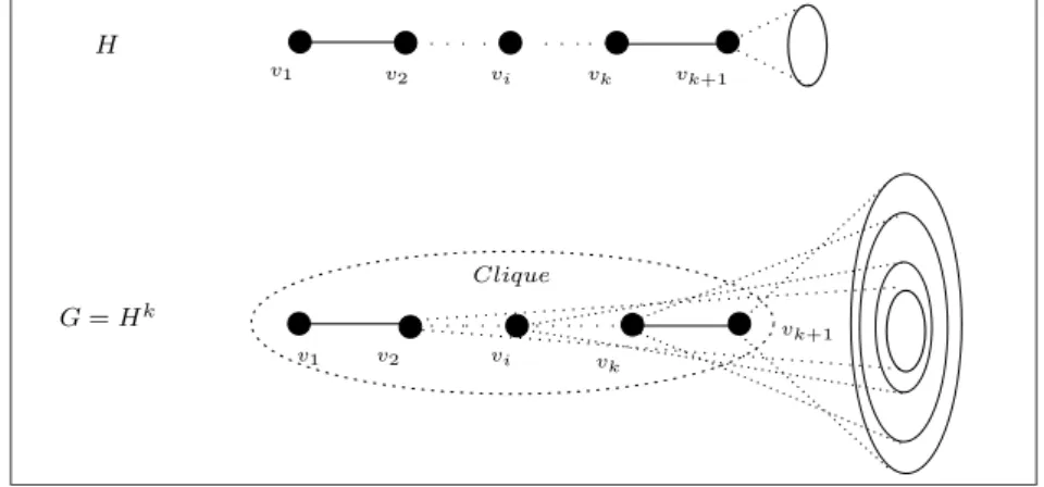
In this example,S1 ={u1, u2, u3} and S2 ={u4, u5, u6, u7} is a possible solution. We also apply the tail structure of a vertex v, first described in [55], and gener-alized later in [45]. The tail structure of a vertex v enables us to pin down exactly the neighborhood ofv in any k-th root H of G.

Lemma 3.2.1 ([55]) Let a, b, c be vertices of a graph G such that

• the only neighbors of a are b and c,

(26)

• cand d are adjacent.

Then the neighbors, in VG− {a, b, c}, of d in any square root of G are the same as

the neighbors, in VG− {a, b, d}, of c in G; see Figure 3.1.

a b c d a b c d

Figure 3.1: Tail inH (left) and in G=H2 _(right)

Lemma 3.2.2 ([45]) Let G= (VG, EG) be a connected graph with {v1, . . . , vk+1} ⊂ VG where NG(v1) = {v2, . . . , vk+1} and NG(vi)⊂ NG[vi+1] for all 1≤ i ≤ k. Then

in any k-th root H of G,

• NH(v1) ={v2},

• NH(vi) ={vi−1, vi+1} for all 2≤i≤k,

• NH(vk+1)−vk =NG(v2)− {v1, . . . , vk+1}.

The vertices v1, . . . , vk are “tail vertices” of vk+1; see Figure 3.2 for an illustration.

vk v1 v2 vi G=Hk v1 H vi v2 vk vk+1 Clique vk+1

Figure 3.2: Tail in k-th rootH of G and in G

We remark that k-th power of _C-graph _{is obviously in NP whenever}

recog-nizingC is polynomially because guessing a k-th root H, verifying if H is in C and checking if G =Hk _{can be done in polynomial time. This is the case for all graph}

(27)

In our reductions we say that vertex u reaches v in k steps if u has a path in H of length at mostk tov. Moreover, we say also that ureaches v inexactly k steps, meaning u has a path inH of length k to v.

(28)

Chapter 4 Powers of Bipartite and Chordal

Graphs

In this chapter, we first prove that both Conjectures 2.2.1 and 2.2.2 are indeed true. Next, in Section 4.2 we show that recognizing k-th powers of chordal graphs is NP-complete.

Finally, in Section 4.3 we provide a reduction to prove the NP-completeness of findingk-th roots of chordal graphs.

4.1 Powers of bipartite graphs

This section shows that the following are NP-complete. k-th power of bipartite graph

Question: Is there a bipartite graphH such that G=Hk_?

k-th power of graph

Question: Is there a graphH such that G=Hk_?

We prove that for fixedk ≥3,k-th power of bipartite graphis NP-complete by reducing set splitting _{to it.}

Our reduction generalizes the one in [45] for cube of bipartite graph. Let S={u1, . . . , un},D={d1, . . . , dm}wheredj ⊆S, 1≤j ≤m, be an instance of set

splitting, and letk≥3 be a fixed integer. We construct an instance G=G(D, S) fork-th power of bipartite graph as follows.

The vertex set ofG consists of:

• Ui, for all 1 ≤i ≤n. Each ‘element vertex’ Ui corresponds to the element ui

(29)

inS.

• Dj, for all 1≤ j ≤ m. Each ‘subset vertex’ Dj corresponds to the subset dj

inD.

• D1

j, . . . , Djk, for all 1≤j ≤m. k ‘tail vertices’Dj1, . . . , Dkj of the subset vertex

Dj.

• P1

1, . . . , P1k−2 and P21, . . . , P2k−2 are k−2 pairs of ‘partition vertices’.

• Connection vertex: X.

The edge set ofG consists of:

• Edges of tail vertices:

(E1) Dj, D1j, . . . , Djk form a clique;

(E2) For all 1 ≤t≤k−1: Dt

j ↔ {Ui |ui ∈dj,1≤i≤n};

j ↔X, Djt ↔ {Dj′ |d_j∩d_j′ 6=∅}, Dt j ↔ {P1h |1≤h ≤k−t−1} and Dtj ↔ {P2h |1≤h≤k−t−1}; (E4) For all 1 ≤t≤k−3: Djt ↔ {Ui |1≤i≤n}, Dt j ↔ {Dhj′ |1≤h≤k−t−2, dj∩dj′ 6=∅};

j ↔ {Dj′ |1≤j′ ≤m};

j ↔ {Djh′ |1≤h≤k−t−4,1≤j′ ≤m}.

• Edges of subset vertices:

(E7) Dj ↔ {X, P11, . . . , P1k−2, P21, . . . , P2k−2},

Dj ↔ {Ui |1≤i≤n}, Dj ↔ {Dj′ |dj ∩dj′ 6=∅}.

(E8) If k ≥4: Dj ↔ {Dj′ |1≤j′ ≤m}.

• Edges of element vertices:

(E9) U1, . . . , Un form a clique, andUi ↔ {X, P₁1, . . . , P₁k−2, P₂1, . . . , P₂k−2}.

• Edges of partition vertices:

(E10) P1

1, . . . , P

k−2

1 , X, U1, . . . , Un form a clique;

P1

2, . . . , P2k−2, X, U1, . . . , Un form a clique.

(E11) For all 1≤t≤k−3,P1t↔ {P2h |1≤h≤k−t−2}, Pt

(30)

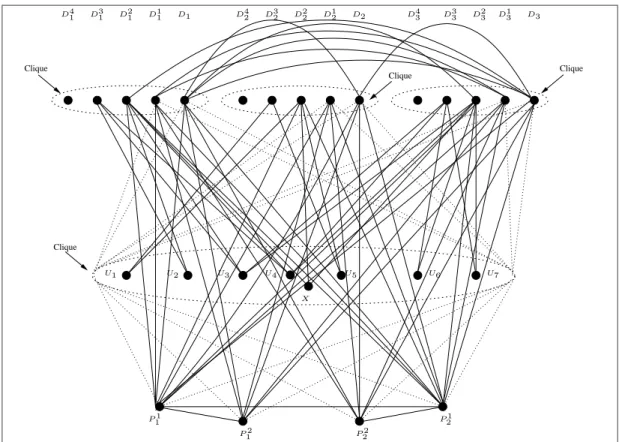
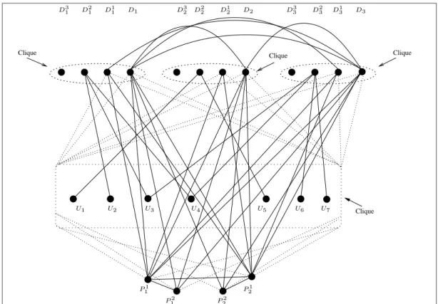
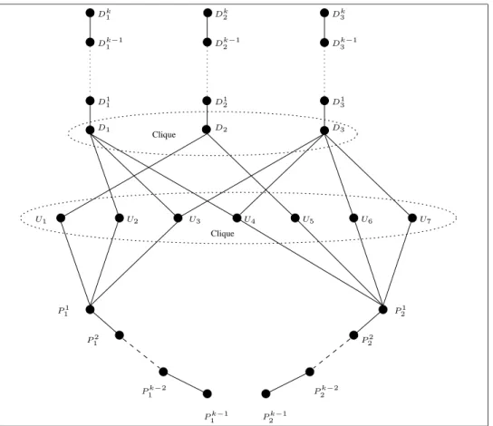
Clique Clique Clique Clique P1 1 P2 1 P22 P1 2 X D3 2 D4 2 D22 D43 D33 D23 D13 D3 D4 1 D31 D21 D11 D1 U₁ U₂ U₃ U₄ U₅ U₆ U₇ D1 2 D2

Figure 4.1: The graphG for the example instance of set splitting _and _k _{= 4}

Clearly, Gcan be constructed from D, S in polynomial time. For an illustration, in case k= 4, the example instance yields the graph G depicted in Figure 4.1. In this and other figures in this chapter, each ellipse corresponds to a clique and we omit the clique edges to keep the figures simpler. The two dotted lines from a vertex to the cliques mean that the vertex is adjacent to all vertices in those cliques. The 4-th root graph H of Gto the solution S1, S2 is shown in Figure 4.2.

Lemma 4.1.1 If there exists a partition of S into two disjoint subsets S1 and S2

such that each subset in D intersects both S1 and S2, then there exists a bipartite

graphH such that G=Hk_.

Proof.LetH have the same vertex set asG. The edges ofH are as follows; see also Figure 4.3.

• Edges of subset vertices and their tail vertices: For all 2≤t ≤k, Dt j ↔D

t−1

j

and D1

j ↔Dj, and Dj ↔ {Ui |ui ∈dj,1≤i≤n}.

• Edges of partition vertices: P1 1 ↔ {Ui |ui ∈S1,1≤i≤n} and P21 ↔ {Ui |ui ∈S2,1≤i≤n}, and for all 2≤t ≤k−2, Pt 1 ↔P t−1 1 and P2t↔P t−1 2 .

(31)

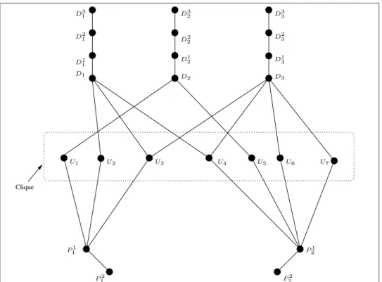
• Edges of connection vertex: X ↔ {U1, . . . , Un}. D4 1 D3 1 D1 1 D4 2 D3 2 D1 2 D4 3 D3 3 D1 3 U2 U4 U5 U6 D1 D2 D3 U1 U3 X P₂1 P₁1 D2₁ D2₂ D2₃ P2 1 P 2 2 U7

Figure 4.2: The bipartite 4-th root graph H of G to the solution S1, S2 Now we verify that the edge set ofHk _{is equal to the edge set of}_{G. We do this by}

following the order of the presentation of the edge set of G; cf. (E1) – (E11). For Dk

j, it is clear that Dj, D1j, . . . , Djk form a clique in Hk for all j, hence

NHk(D_jk) =N_G(Dk_j).

For 1 ≤ t ≤ k−1, the vertex Dt

j reaches Dj in t steps. By the construction of

H, Dj ↔ Ui whenever ui ∈ dj. Thus within t+ 1 steps, Dtj reaches Ui whenever

ui ∈ dj, therefore Djt ↔ Ui in Hk whenever ui ∈ dj. By comparing with (E2), NHk(D_jt) =N_G(D_jt).

For 1≤t≤k−2, the vertex Dt

j reaches Dj int steps. Since Dj ↔Ui whenever

ui ∈dj and for alli,Ui ↔XinH, so withinksteps,DjtreachesUiwheneverui ∈dj,

and Dt

j reaches X. Also, in H, Dj reaches Dj′ in two steps whenever d_j ∩d_j′ 6=∅,

thus within k steps, Dt

j reaches Dj′ whenever d_j ∩d_j′ 6= ∅. Furthermore, since

we have a solution for set splitting, every Dj has a common neighbor with P11 and a common neighbor with P1

2. So Djt reaches P11, . . . , P k−t−1 1 and Dtj reaches P1 2, . . . , P k−t−1

2 withink steps. By comparing with (E3), NHk(D_jt) =N_G(D_jt). For 1 ≤ t ≤ k−3, the vertex Dt

j reaches Dj in t steps. Moreover, Dj reaches

Ui within three steps for all i. So Dtj reaches Ui within k steps for all i. Also,

(32)

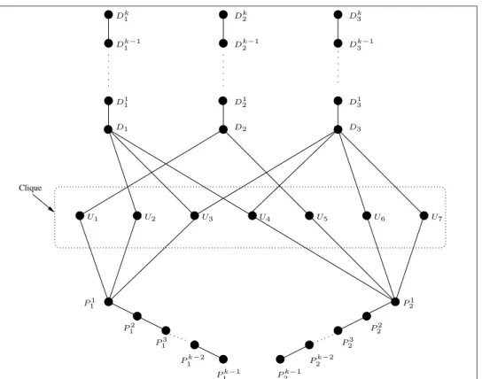
Dk₁ Dk−1 1 D1 1 Dk₂ Dk−1 2 D1 2 Dk₃ Dk−1 3 D1 3 U4 U5 U6 P₁1 P₂1 P2 2 P3 2 Pk−2 2 Pk−2 1 P₁k−3 P₂k−3 P3 1 P2 1 D1 D2 D3 U1 U3 X U2 U7

Figure 4.3: A bipartite k-th rootH in Lemma 4.1.1 to the example solution S1, S2

D1

j′, . . . , D

k−t−2

j′ wheneverdj∩dj′ 6=∅. By comparing with (E4), for all 1≤t ≤k−3,

NHk(D_jt) =N_G(D_jt).

For 1 ≤t≤ k−4, the vertex Dt

j reaches Dj int steps. Also, Dj reaches Dj′ for

allj 6= j′ _{in only four steps, thus within} _k _steps, _Dt

j reaches Dj′ for all j 6=j′. By

comparing with (E5), for all 1≤t≤k−4,NHk(Dt_j) =N_G(Dt_j). For 1 ≤t≤ k−5, the vertex Dt

j reaches Dj int steps. Also, Dj reaches D1j′ for

allj 6= j′ _{in only five steps, thus within} _k _steps, _Dt

j reaches D1j′, . . . , D

k−t−4

j′ for all

j 6=j′_{. By comparing with (E}

6), for all 1≤t ≤k−5, NHk(D_jt) =N_G(D_jt).

Next, the vertex Dj reaches Ui in one step whenever ui ∈ dj. In H, X ↔ Ui,

so within k steps, Dj reaches X and Dj reaches Ui for all i. Moreover, since we

have a solution forset splitting, every Dj has a common neighbor withP11 and a common neighbor with P1

2. In H, {P11, . . . , P

k−2

1 } and {P21, . . . , P

k−2

2 } are paths of lengthk−3. Thus, within k steps, Dj reaches P11, . . . , P1k−2, P21, . . . , P2k−2. Also, it is clear thatDj reaches Dj′ in only two steps whenever d_j∩d_j′ 6=∅. Furthermore,

if k ≥ 4, Dj and Dj′ reach X in two steps, therefore Dj is adjacent to Dj′ for all

j 6=j′_{. By comparing with (E}

7) and (E8),NHk(D_j) =N_G(D_j).

Now consider Ui. In H, Ui ↔ X, hence U1, . . . , Un form a clique in Hk.

(33)

and {P11, . . . , P1k−2} and {P21, . . . , P2k−2} are paths of length k −3 in H. Thus, within k steps Ui reaches P11, . . . , P1k−2, P21, . . . , P2k−2. By comparing with (E9), NHk(U_i) =N_G(U_i) for all i.

Finally, for partition vertices, it is clear that P1

1, . . . , P1k−2, X, U1, . . . , Un form

a clique in Hk _and _P1

2, . . . , P2k−2, X, U1, . . . , Un form a clique in Hk. Moreover,

for all 1 ≤ t ≤ k−3, since P1

1 and P21 have at least one neighbor Ui in H. Also,

since Ui ↔ X in H, P1t reaches P21, . . . , P2k−t−2 and P2t reaches P11, . . . , P1k−t−2. By comparing with (E10) and (E11),NHk(Pt

1) = NG(P1t) and NHk(Pt

2) = NG(P2t) ∀t. We have checked that the edge set of Hk _{is equal to the edge set of} _G.

Now we will show thatH is a bipartite graph. We do this by showing a 2-coloring of H. The vertices get color 1 consist of Dj, Dj2, . . . , D

2⌊k 2⌋ j , X, P11, . . . , P 2⌊k−3 2 ⌋+1 1 , P1 2, . . . , P 2⌊k−3 2 ⌋+1

2 . The other vertices of H get color 2. It is easy to check that vertices in the same color class are not adjacent. This completes the proof of

Lemma 4.1.1.

For the example instance, the k-th root graph H corresponds to the solution S1, S2 is shown in Figure 4.3.

Now we show that if G has a k-th root H (not necessarily bipartite), then there is a partition of S into two disjoint subsets S1 and S2 such that each subset in D intersects both S1 and S2. We first need:

Proposition 4.1.2 If H is a k-th root of G, then, in H:

(i) For all i, j: Dj is only adjacent to Ui whenever ui ∈dj;

(ii) Dk

j is only adjacent to Djk−1, Dj1 is only adjacent to Dj and D2j, and Dtj is

only adjacent to Dtj−1 and D t+1

j , 2≤t≤k−1;

(iii) If k ≥4, P_ℓk−2 is only adjacent to P_ℓk−3, and for all 2≤t≤k−3: Pt

ℓ is only

adjacent to Pℓt−1 and P t+1

ℓ , ℓ= 1,2.

Proof. By the construction of G, we have for all j: NG(Djk) = {Dj, D1j, . . . , D k−1

j },

NG(D1j)⊂NG[Dj] andNG(Djt)⊂NG[Djt−1] for all 2≤t ≤k−1. Thus, (i) and (ii)

follow immediately from Lemma 3.2.2.

For (iii), we only verify forℓ = 1; the caseℓ= 2 is similar. Since G=Hk _{and by}

the construction ofG, and by (i), (ii), we have for all i, j: dH(Dkj−2, P

h

1)> k for 2≤h ≤k−2. (4.1)

dH(P1k−2, X)≥k−3, dH(P1k−2, Ui)≥k−2. (4.2)

(34)

Since NG(P1k−2) =NHk(Pk−2 1 ) ={P11, . . . , P1k−3, X, U1, . . . , Un, D1, . . . , Dm, D11, . . . , D1m} and NHk−3(Pk−2 1 ) = NH1(P k−2 1 )∪NH2(P k−2 1 )∪. . .∪N k−3 H (P k−2 1 ), it follows from (4.2) and (4.3):

{P11, . . . , P1k−3} ⊆NHk−3(P₁k−2)⊆ {P₁1, . . . , P₁k−3, X}. Case 1: NHk−3(Pk−2 1 ) ={P11, . . . , P k−3 1 }. That is, N1 H(P k−2 1 )∪NH2(P k−2 1 )∪. . .∪NHk−3(P k−2 1 ) = {P11, . . . , P1k−3}. Note that Nt H(P k−2

1 ) 6= ∅ for 1 ≤ t ≤ k−3: Otherwise, let u be a vertex in G such that dH(u, P₁k−2) > k, then there is no path between u and P₁k−2 in H and thus there

is also no path between u and Pk−2

1 in G which contradicts to the fact that G is connected. Therefore,

N_Ht (P₁k−2)

= 1 for 1≤t ≤k−3. Thus, P₁1, . . . , P₁k−3 form

a path of length k−4 in H, say PA. Also, we have the following claims.

Claim 1: P1

1 must be the end-vertex of PA, and P11 must be adjacent to Ui for

some 1≤i≤n.

Proof of Claim 1: Otherwise, let Pt

1 be end-vertex of PA, for t 6= 1. Then, by

NHk₋3(P₁k−2) = {P₁1, . . . , P₁k−3}, hence in H,P₁1 6↔ {X, U1, . . . , U_n, D_j, D1_j, . . . , D_jk},

therefore dH(P1t, Djk−2) ≤ dH(P11, Djk−2) ≤ k (as in G, P11 ↔ Djk−2), which

contra-dicts to (4.1). It is clear that P1

1 must be adjacent to Ui for some 1 ≤ i ≤ n: Otherwise, by in

H, P1

1 6↔ {Dj, D1j, . . . , Djk} and X 6↔ {Dj, Dj1, . . . , Dkj}, hence P11 6↔ Djk−2 in G,

contradicting to the construction of G.

Claim 2: Pk−3

1 must be the end-vertex of PA, and P1k−3 must be adjacent to P₁k−2.

Proof of Claim 2: Otherwise, let Pt′

1 be end-vertex of PA, for t′ 6=k−3. Then, by

the Claim 1, dH(P1k−3, Dj3) ≤ dH(P1k−3, P11) +dH(P11, D3j) ≤ (k−5) + 5, therefore,

Pk−3

1 ↔D3j in G, contradicting to the construction of G.

It is clear that Pk−3

1 must be adjacent to P1k−2: Otherwise, then dH(P1k−2, P11) ≤ k − 4, hence dH(P₁k−2, D2j) ≤ k, which contradicts the fact that, in G, P

k−2 1 is non-adjacent toD2

j.

Claim 3: Pt

1 is only adjacent to P1t−1 and toP1t+1 for all 2≤t ≤k−3.

Proof of Claim 3: By the Claim 2, N1

H(P k−2

1 ) = {P1k−3} and NHk−3(P k−2

1 ) = {P11}. Next, P₁k−3 must be adjacent to P₁k−4: Otherwise, dH(P₁k−3, P₁1) ≤ k − 5, hence

dH(P1k−3, D3j) ≤ (k−5) +dH(P11, Dj3)≤ k, contradicting the fact that, in G, P k−3 1 is non-adjacent toD3

j.

By the same argument, we can show that Pk−4

1 must be adjacent to P1k−5, . . ., P12 must be adjacent to P1

1, i.e., for all 2≤t ≤ k−3,P1t is only adjacent to P

t−1

1 and

(35)

Case 2_: _N_Hk−3(P₁k−2) ={P₁1, . . . , P₁k−3, X}. Then by (4.2), dH(P1k−2, X) = k −3, hence X ∈ B := NHk−3(P k−2 1 ). Set A := S 1≤t≤k−4N t H(P k−2

1 ), and note that NHt(P k−2

1 )6= ∅ for 1 ≤ t ≤ k−3, hence |A| ≥ k−4, and 1 ≤ |B| ≤2.

Subcase 2.1: B = {X, P1t0} for some 1 ≤ t0 ≤ k−3. In this case, A contains the k−4 vertices Pt

1, for 1≤t ≤k−3, t6=t0. Similar to Case 1, it can be shown that P1

1, . . . , P

k−2

1 form a path of length k−3 in H with end-vertices P11 and P

k−2 1 .

Subcase 2.2: B = {X}. That is, N1

H(P k−2 1 )∪. . .∪N k−4 H (P k−2 1 ) = {P11, . . . , P k−3 1 }. Note that, Nt H(P k−2

1 ) 6= ∅ for 1 ≤ t ≤ k −3, therefore there is uniquely a set N_Ht0(Pk−2

1 ) for some 1 ≤ t0 ≤ k −4 such that N

t0 H(P k−2 1 ) = {Pt a 1 , P tb 1 } for some 1≤ta, tb ≤k−3. LetC := S 1≤t≤k−4,t6=t0N t H(P k−2

1 ) containingk−5 vertices exactly of {Pt 1 | 1 ≤ t ≤ k −3, t 6∈ {ta, tb}}. By NHt(P k−2 1 ) 6= ∅ for 1 ≤ t ≤ k − 3, hence N_Ht(P₁k−2)

= 1 for 1 ≤ t ≤ k − 3 and t 6∈ {ta, tb}. Therefore, P1t for all 1 ≤ t ≤ k − 3 and t 6∈ {ta, tb}, form a path of length k −6 in H. Since

Pta 1 , P tb 1 ∈N t0 H(P k−2

1 ) for some 1≤t0 ≤k−4, hencedH(P₁1, P₁k−2)≤k−4. Therefore,

dH(P1k−2, D2j) ≤ dH(P1k−2, P11) +dH(P11, D2j) ≤ (k−4) + 4, this contradicts to the

fact that, in G, Pk−2

1 is non-adjacent toD2j.

Thus, Subcase 2.2 cannot occur.

Now we are ready to prove the reverse direction.

Lemma 4.1.3 If H is a k-th root of G, then there exists a partition of S into two disjoint subsets S1 and S2 such that each subset in D intersects both S1 and S2.

Proof. From Proposition 4.1.2 and the fact that, in G, P1 1 6↔ P k−2 2 , P21 6↔ P k−2 1 , it follows that, in H, P1

1 are not adjacent to P21, . . . , P

k−2

2 and P21 are not adjacent toP1

1, . . . , P1k−2. Also, since, in G, P11 6↔ Djk−1 and P21 6↔ Dkj−1, it follows that, in

H, P1

1 and P21 are not adjacent to the tail vertices and the subset vertices. Thus, S1 =NH(P₁1)\ {X, P₁2, . . . , P₁k−2} and S2 =NH(P₂1)\ {X, P₂2, . . . , P₂k−2} consist of

element verticesonly. We will show thatS1 and S2 define a desired partition of the element set S.

Claim 1: S1∩S2 =∅.

Proof of Claim 1: In case k = 3, by the construction of G, P1

1 is non-adjacent to P1

2 in G, therefore P11 and P21 have no common element neighbor in H, thus S1∩S2 =∅.

Let k ≥ 4, by Proposition 4.1.2 (iii), {P1

ℓ, . . . , P k−2

ℓ } form an induced path in H

of length k−3, ℓ = 1,2. Thus, if P1

1 and P21 have a common neighbor in H then Pk−2

2 reaches P11 ink−3 + 1 + 1 steps, which contradicts to the fact that, in G,P11 is non-adjacent toPk−2

2 .

(36)

Proof of Claim 2: Since the partition vertices P11 and P21 are adjacent to all subset verticesDk−2

j inG, and by Proposition 4.1.2,Dk−2 reachesDj in exactlyk−2 steps,

P1

1 and P21 must reachDj inexactly two steps and thus each ofP₁1, P₂1 must have a

common neighbor withDj in the element set for all j, i.e., NH(P11)∩NH(Dj)6=∅

and NH(P21)∩ NH(Dj) 6= ∅ for all 1 ≤ j ≤ m. That means, each subset in D

intersects both S1 and S2.

By Claim 1 and Claim 2, S1 and S2 are actually the desired partition of S. Notice that in the Lemma 4.1.3, we did not use the property thatH is a bipartite graph. In fact, any k-th root of G would tell us how to do set splitting. In particular,any bipartitek-th rootH ofGwill do. Hence, by Lemmas 4.1.1 and 4.1.3, we conclude

Theorem 4.1.4 For any fixed k ≥3, k-th power of bipartite graph is NP-complete.

By the same reason, k-th power of C-graph is NP-complete for all fixed k ≥ 3 wheneverC contains all bipartite graphs (such as triangle-free graphs, parity graphs, perfect graphs, etc.). In particular, applied for the class of all graphs, this observa-tion and the NP-completeness of square of graph [55] together give

Theorem 4.1.5 For all fixed k ≥2, k-th power of graph is NP-complete.

4.2 Powers of chordal graphs

Lau and Corneil [46] shown that square of chordal graph is NP-complete. In this section we extend that result by showing that k-th power of chordal graph is NP-complete for all fixed k ≥ 3. We will reduce set splitting to it as follows.

Let S = {u1, . . . , un}, D = {d1, . . . , dm} where dj ⊆ S, 1 ≤ j ≤ m, be an

instance of set splitting_{, and let} _k _≥ _{3 be a fixed integer. We construct an}

instance G=G(D, S) for k-th power of chordal graph as follows. The vertex set ofG consists of:

• Ui, 1≤i≤n. Each ‘element vertex’ Ui corresponds to the element ui inS.

• Dj, 1≤j ≤m. Each ‘subset vertex’ Dj corresponds to the subsetdj in D.

• D1

j, . . . , Djk, 1≤j ≤m. k ‘tail vertices’ D1j, . . . , Djk of the subset vertex Dj.

• P1

1, . . . , P

k−1

1 and P21, . . . , P

k−1

2 are k−1 pairs of ‘partition vertices’. The edge set ofG consists of:

(37)

• Edges of tail vertices: (T1) Dj, D1j, . . . , Djk form a clique. (T2) For all 1≤t≤k−1,Dt j ↔ {Ui |ui ∈dj,1≤i≤n}. (T3) For all 1≤t≤k−2,Dt j ↔ {Ui |1≤i≤n}, Djt ↔ {Dj′ |d_j∩d_j′ 6=∅}, Dt j ↔ {P1h |1≤h ≤k−t−1} and Dtj ↔ {P2h |1≤h≤k−t−1}. (T4) For all 1≤t≤k−3,Dt j ↔ {Dj′ |1≤j′ ≤m}; Dt j ↔ {Dhj′ |1≤h≤k−t−2, dj∩dj′ 6=∅}. (T5) For all 1≤t≤k−4,Dtj ↔ {Dhj′ |1≤h≤k−t−3,1≤j′ ≤m}.

• Edges of subset vertices:

(T6) Dj ↔ {P11, . . . , P1k−1, P21, . . . , P2k−1},Dj ↔ {Ui |1≤i≤n}, and

Dj ↔ {Dj′ |1≤j′ ≤m}.

• Edges of element vertices:

(T7) U1, . . . , Un form a clique, andUi ↔ {P11, . . . , P1k−1, P21, . . . , P2k−1}.

• Edges of partition vertices:

(T8) P11, . . . , P1k−1, U1, . . . , Un form a clique,

P1

2, . . . , P

k−1

2 , U1, . . . , Un form a clique.

(T9) For all 1≤t≤k−2,Pt

1 ↔ {P2h |1≤h≤k−t−1} and Pt

2 ↔ {P1h |1≤h≤k−t−1}.

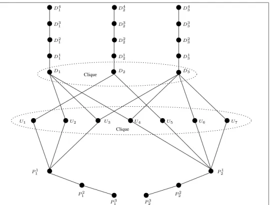
Clearly, Gcan be constructed from D, S in polynomial time. For an illustration, in case k = 3, the example instance yields the graph G is depicted in Figure 4.4. While the corresponding cube root graph H to the solution S1, S2 is shown in Figure 4.5.

Lemma 4.2.1 If there exists a partition of S into two disjoint subsets S1 and S2

such that each subset in D intersects both S1 and S2, then there exists a chordal

graphH such that G=Hk_.

Proof.LetH have the same vertex set asG. The edges ofH are as follows; see also Figures 4.6.

• Edges of subset vertices and their tail vertices: For all 2≤t ≤k, Dt j ↔D

t−1

j

and D1

j ↔Dj, and Dj ↔ {Ui |ui ∈dj,1≤i≤n}.

• Edges of element vertices: U1, . . . , Un form a clique.

• Edges of partition vertices: P1 1 ↔ {Ui |ui ∈S1,1≤i≤n}, and P21 ↔ {Ui |ui ∈S2,1≤i≤n}, and for all 2≤t ≤k−1, Pt 1 ↔P t−1 1 and P2t↔P t−1 2 .

(38)

Clique

Clique _Clique Clique

P₂1 P₁1 P₁2 P₂2 U3 U1 U2 U4 U5 U6 U7 D3 1 D12 D11 D1 D32 D22 D12 D2 D33 D32 D13 D3

Figure 4.4: The graphG for the example instance of set splitting and k = 3

Similar to the proof of Lemma 4.1.1 we can show that Hk ₌ _G _{by following the}

order of the presentation of the edge set ofG; cf. (T1) – (T9), as follows. For Dk

j, it is clear that Dj, Dj1, . . . , Dkj form a clique in Hk for all j, hence

NHk(D_jk) =N_G(Dk_j).

j reachesDj inH int steps. By the construction

of H, Dj ↔Ui whenever ui ∈dj. Thus within t+ 1 steps, Djt reaches Ui whenever

ui ∈ dj, therefore Djt ↔ Ui in Hk whenever ui ∈ dj. By comparing with (T2), NHk(D_jt) =N_G(D_jt).

j reaches Dj int steps. Since Dj ↔Ui whenever

ui ∈ dj and U1, . . . , Un form a clique in H. Thus within t + 2 steps, Djt reaches

Ui for all i, therefore Dtj ↔ Ui in Hk for all i. Also, in H, Dj reaches Dj′ in two

steps whenever dj ∩dj′ 6=∅, thus within t+ 2 ≤k steps, D_jt reaches D_j′ whenever

dj ∩dj′ 6= ∅. Furthermore, since we have a solution for set splitting, every D_j

has a common neighbor to P1

1 and a common neighbor to P21. Moreover, in H,

{P1

1, . . . , P1k−1} and {P21, . . . , P2k−1} are induced path of length k−2, therefore Dtj

reachesP1

1, . . . , P1k−t−1 andDjtreachesP21, . . . , P2k−t−1withinksteps. By comparing with (T3),NHk(Dt_j) = N_G(Dt_j).

For 1 ≤ t ≤ k−3, the vertex Dt

(39)

Clique D₁3 D2 1 D₁1 P1 1 P21 P2 1 P 2 2 U6 U5 U3 U2 U1 D1 D3₂ D2 2 D1₂ D2 D3₃ D2 3 D1₃ D3 U7 U4

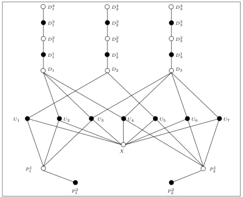
Figure 4.5: Cube root graph H to the solution S1,S2.

Dj′ within three steps for all j′. So within t+ 3≤k steps, Dt_j reaches Dj′ for all j′,

thereforeDt

j ↔Dj′ for allj′. Furthermore, as D_j reachesD_j′ in two steps whenever

dj∩dj′ 6=∅, thus withink steps, D_jt reaches D_j1′, . . . , D

k−t−2

j′ wheneverdj∩dj′ 6=∅.

By comparing with (T4), NHk(D_jt) =N_G(D_jt). For 1 ≤t≤ k−4, the vertex Dt

j reaches Dj int steps. Also, Dj reaches Dj′ for

allj′ _{in three steps, therefore within} _k _steps, _Dt

j reaches Dj1′, . . . , D

k−t−3

j′ for all j

′_.

By comparing with (T5), NHk(D_jt) =N_G(D_jt).

Next, the vertex Dj reaches Ui in one step whenever ui ∈ dj. In H, U1, . . . , Un

form a clique, so within k steps, Dj reaches Ui for all i and Dj reaches Dj′ for

all j′_{. Moreover, since we have a solution for} _{set splitting}_{, every} _D

j has a

common neighbor to P1

1 and a common neighbor toP21. In H, {P11, . . . , P1k−1} and

{P1

2, . . . , P2k−1} are induced path of length k−2. Thus, within k steps, Dj reaches

P1 1, . . . , P k−1 1 , P21, . . . , P k−1 2 . By comparing it with (T6),NHk(D_j) = N_G(D_j). For Ui, U1, . . . , Un form a clique in H, hence U1, . . . , Un form also a clique in

Hk_{. In} _H, _U

i ↔ P₁1 whenever ui ∈ S1, and Ui ↔ P₂1 whenever ui ∈ S2.

More-over, P1

1, . . . , P1k−1 form an induced path of length k −2 in H and P21, . . . , P2k−1 form an induced path of length k − 2 in H. Thus, within k steps Ui reaches

P1 1, . . . , P k−1 1 , P21, . . . , P k−1 2 .

(40)

Finally, for partition vertices, it is clear that P11, . . . , P1k−1, U1, . . . , Un form a

clique in Hk _and _P1

2, . . . , P2k−1, U1, . . . , Un form a clique in Hk. Moreover, for all

1 ≤ t ≤ k −2, since P1

1 and P21 have at least one neighbor Ui in H. Also, since

U1, . . . , Un form a clique in H, P1t↔ {P21, . . . , P2k−t−1} and P2t↔ {P11, . . . , P1k−t−1}. By comparing with (T8) and (T9), NHk(Pt

1) = NG(P1t) and NHk(Pt

2) =NG(P2t) for allt.

We checked that the edge set of Hk _{is equal to the edge set of} _G.

Now to complete the proof we will show that H is a chordal graph. We do this by giving a simplicial elimination ordering ofH.

First of all, allDk

j are simplicial inH and we eliminate them first. Then for each

vertex of Djk−1, . . . , D1j, its neighbors in the remaining vertices of H form a clique.

So we can eliminate Djk−1, . . . , Dj1 for all 1 ≤ j ≤ m. By the same reason, each

partition vertex of sets{Pk−1

1 , . . . , P12}and {P2k−1, . . . , P22}is also simplicial and we eliminate them.

Next, since the element vertices U1, . . . , Un induce a complete subgraph.

More-over, Dj,P₁1 andP₂1 have only neighbors in the element set {U1, . . . , Un}, therefore,

Dj, P11 and P21 are also simplicial in the subgraphs induced by remaining vertices of H and we can eliminate them. Finally, the element vertices U1, . . . , Un are

remaining vertices; they induce a complete subgraph and this completes the proof

that H is chordal.

Now we show that ifG has a k-th root H ( not necessarily chordal ), then there is a partition of S into two disjoint subsets S1 and S2 such that each subset in D intersects both S1 and S2. Similar to the proof of Lemma 4.1.3, we first need:

Proposition 4.2.2 If H is a k-th root of G, then, in H:

(i) For all i, j: Dj is only adjacent to Ui whenever ui ∈dj;

(ii) Dk

j is only adjacent to D

k−1

j , Dj1 is only adjacent to Dj and D2j, and Dtj is

only adjacent to Dtj−1 and D t+1

j for 2≤t≤k−1;

(iii) Pk−1

ℓ is only adjacent to P

k−2

ℓ , and for all 2≤t ≤k−2: Pℓt is only adjacent

to Pt−1

ℓ and P t+1

ℓ for ℓ= 1,2.

Proof. By the construction of G, we have for all j: NG(Djk) = {Dj, D1j, . . . , D k−1

j },

NG(D1j)⊂NG[Dj] andNG(Djt)⊂NG[Djt−1] for all 2≤t ≤k−1. Thus, (i) and (ii)

follow immediately from Lemma 3.2.2.

For (iii), we only verify forℓ = 1; the caseℓ= 2 is similar. Since G=Hk _{and by}

the construction ofG, and by (i), (ii), we have for all i, j: dH(Djk−2, P

t

(41)

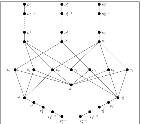
Clique Dk₁ Dk−1 1 D1 1 U1 U2 U3 U4 U5 U6 P₁1 P₂1 P2 2 P3 2 Pk−1 2 Pk−1 1 P₁k−2 P₂k−2 P3 1 P2 1 D1 U7 Dk₂ Dk−1 2 D1 2 D2 Dk₃ Dk−1 3 D1 3 D3

Figure 4.6: A chordal k-th root H in Lemma 4.2.1 to the example solution S1, S2 dH(P1k−1, Ui)≥k−1, dH(P1k−1, Dj)≥k. (4.5) Since NG(P₁k−1) =NHk(Pk−1 1 ) ={P11, . . . , P k−2 1 , U1, . . . , Un, D1, . . . , Dm} and NHk₋2(P₁k−1) = N_H1(P₁k−1)∪N_H2(P₁k−1)∪. . .∪N_Hk−2(P₁k−1), it follows from (4.5): NH1(P k−1 1 )∪NH2(P k−1 1 )∪. . .∪N k−2 H (P k−1 1 ) ={P11, . . . , P k−2 1 }. Note thatNt H(P k−1

1 )6=∅ for 1≤t ≤k−2 (otherwise, let u be a vertex in G such that dH(u, P1k−1) > k, then there is no path between u and P1k−1 in H and thus there is also no path between u and P₁k−1 in G which contradicts to the fact that Gis connected), hence

N_Ht (P₁k−1)

= 1 for 1≤ t≤ k−2. Therefore, P₁1, . . . , P₁k−2

form a path of lengthk−3 in H, say PB. Moreover, we have the following claims.

Claim 1: P1

1 must be the end-vertex of PB, also P11 must be adjacent to Ui for

some 1≤i≤n.

Proof of Claim 1: Otherwise, let Pt

1 be end-vertex of PB, for some 2 ≤

t ≤ k − 2. Then, by NHk−2(P₁k−1) = {P1

1, . . . , P

k−2

(42)

{U1, . . . , Un, Dj, D1j, . . . , Djk}, therefore dH(P1t, Djk−2) ≤ dH(P11, Djk−2) ≤ k (as in

G,P1 1 ↔D

k−2

j ), which contradicts (4.4).

Moreover, it is clear thatP1

1 must be adjacent to Ui for some 1≤i≤n: Otherwise,

by in H, P1

1 6↔ {Dj, D1j, . . . , Djk}, hence P11 6↔ Dkj−2 in G, contradicting to the

construction ofG.

Claim 2: Pk−2

1 must be the end-vertex of PB, also P1k−2 must be adjacent to P₁k−1.

Proof of Claim 2: Otherwise, let Pt′

1 be end-vertex of PB, for some 1≤ t′ ≤ k−3.

Then, by the Claim 1, dH(P1k−2, Dj2) ≤ dH(P1k−2, P11) +dH(P11, D2j) ≤ (k−4) + 4,

therefore,Pk−2

1 ↔Dj2 inG, contradicting to the construction of G; cf. (T3).

Also, it is clear thatP₁k−2must be adjacent toP₁k−1: Otherwise, thendH(P1k−1, P11)≤ k−3, hence dH(P₁k−1, Dj1)≤k, which contradicts the fact that, in G, P

k−1

1 is non-adjacent toD1

j.

Claim 3: Pt

1 is only adjacent to P1t−1 and toP1t+1 for all 2≤t ≤k−2.

Proof of Claim 3: By the Claim 2, N1

H(P k−1

1 ) = {P1k−2} and NHk−2(P k−1

1 ) = {P11}. Next, P₁k−2 must be adjacent to P₁k−3: Otherwise, dH(P₁k−2, P₁1) ≤ k − 4, hence

dH(P1k−2, D2j) ≤ (k−4) +dH(P11, Dj2)≤ k, contradicting the fact that, in G, P k−2 1 is non-adjacent toD2

j.

By the same argument, we can show that Pk−3

1 must be adjacent to P1k−4, . . ., P12 must be adjacent to P1

1, therefore for all 2≤t≤k−2,P1t is only adjacent to P

t−1 1

and toP1t+1.

Now we are ready to prove the reverse direction.

Lemma 4.2.3 If H is a k-th root of G, then there exists a partition of S into two disjoint subsets S1 and S2 such that each subset in D intersects both S1 and S2.

Proof. From Proposition 4.2.2 and the fact that, in G, P1

1 6↔ P2k−1, P21 6↔ P1k−1, it follows that, in H, P1

1 is not adjacent to P21, . . . , P

k−1

2 and P21 is not adjacent to P1

1, . . . , P1k−1. Also, since, in G, P11 6↔ Djk−1 and P21 6↔ Djk−1, it follows that,

in H, P1

1 and P21 are not adjacent to the tail vertices and the subset vertices. Thus, S1 =NH(P₁1)\ {P₁2, . . . , P₁k−1} and S2 =NH(P₂1)\ {P₂2, . . . , P₂k−1}consist of

element verticesonly. We will show thatS1 and S2 define a desired partition of the element set S.

Claim 1: S1∩S2 =∅.

Proof of Claim 1: By Proposition 4.2.2 (iii), {P1

ℓ, . . . , P k−1

ℓ } form an induced path

in H of length k−2, ℓ = 1,2. Thus, if P1

1 and P21 have a common neighbor in H thenP1

1 reaches P2k−1 in k−2 + 1 + 1 steps, this contradicts to the fact that, in G, P1

1 is non-adjacent to P2k−1.

Graph Powers: Hardness Results, Good Characterizations and Efficient Algorithms. Dissertation

Hardness Results,

Good Characterizations and

Efficient Algorithms

Dissertation

zur

Erlangung des akademischen Grades

Doktor-Ingenieur (Dr.-Ing.)

der Fakult¨at f¨

ur Informatik und Elektrotechnik

der Universit¨at Rostock

Vorgelegt von

MSc. Ngoc Tuy Nguyen

Rostock, November 2009

Abstract

Acknowledgments

Contents

I

Introduction

1

II

NP-completeness

13

III

Good Characterizations and Efficient Algorithms

60

List of Figures

Part I

Introduction

Chapter 1

Overview

1.1

Introduction

1.2

Contributions of the thesis

Chapter 2

Background

2.1

Definitions and notation

2.2

Graph powers and related works

Part II

NP-completeness

Chapter 3

Preliminaries

3.1

Introduction

3.2

Preliminaries

Chapter 4

Powers of Bipartite and Chordal

Graphs

4.1

Powers of bipartite graphs

4.2

Powers of chordal graphs