AUSTRALIAN JOURNAL OF BASIC AND
Open Access Journal
Published BY AENSI Publication
© 2016 AENSI Publisher All rights reserved
This work is licensed under the Creative Commons Attribution International License (CC BY). http://creativecommons.org/licenses/by/4.0/
To Cite This Article: S. Gilbert Nancy and S. Appavu Alias Balamurugan for Cancer Classification using Gene Expression Data
Feature Selection Technique Based on Neuro
Classification using Gene Expression Data
1S.Gilbert Nancy and 2S. Appavu Alias Balamurugan
1Department of Computer Science and Engineering, Kalasalingam University,
2Professor, Department of Information Technology, K.L.N.College of Information Technology, Madurai, India.
Address For Correspondence:
S.Gilbert Nancy, Department of Computer Science and Engineering, Kalasalingam University, Krishnancoil, Tamilnadu, India. E-mail: [email protected]
A R T I C L E I N F O Article history:
Received 04 December 2015 Accepted 22 January 2016 Available online 14 February 2016
Keywords:
Feature selection, Neuro- fuzzy-rough. FPRS, ANFIS and Microarray data
Microarrays are new technology
great potential to provide accurate medical diagnostics to help and find right treatment for many diseases. It provides a detailed genome-wide molecular portra
2008) are silicon chips that simultaneously measure the mRNA expression levels of tens of thousands of genes. The expression levels of the same sets of genes under study are normally measured from
eventually recorded in a dataset. In a typical microarray data set, each column represents a gene and each row represents a sample. It has three issues, namely: (1) volume
genes; (2) severely limited amount of samples
expense of obtaining microarray samples; and (3) abundance of redundancy among genes. These issues induce severe challenges to the classification tasks. These p
technique, which can found the genes most strongly related to a particular class. Generally speaking, feature selection
1999) (also known as attribute selection) is a process commonly used in machine learning concept, wherein a subset of the features available in the dataset is used to apply for learning algorithm. The best subset contains the least number of dimensions which contributes to a
unimportant dimensions. This is an important stage of preprocessing technique and it is one of the two ways of avoiding the curse of dimensionality (the other is feature extraction).
AUSTRALIAN JOURNAL OF BASIC AND
APPLIED SCIENCES
ISSN:1991-8178 EISSN: 2309-8414 Journal home page: www.ajbasweb.com
rights reserved
This work is licensed under the Creative Commons Attribution International License (CC BY). http://creativecommons.org/licenses/by/4.0/
S. Gilbert Nancy and S. Appavu Alias Balamurugan., Feature Selection Technique Based on Neuro for Cancer Classification using Gene Expression Data. Aust. J. Basic & Appl. Sci., 10(2): 9-17, 2016
Feature Selection Technique Based on Neuro-Fuzzy-Rough Set for Cancer
Classification using Gene Expression Data
Balamurugan
Science and Engineering, Kalasalingam University, Krishnancoil, Tamilnadu, India. Department of Information Technology, K.L.N.College of Information Technology, Madurai, India.
Department of Computer Science and Engineering, Kalasalingam University, Krishnancoil, Tamilnadu, India.
A B S T R A C T
The study of gene expression in cancer diagnosis is done by microarray technology. The description of microarray technology issues (to select the corrective
and curse of dimensionality) and proposed technique to overcome these issues are the scope of this paper. Proposed technique helps to improve the performance of learning models by removing most irrelevant, redundant and noise features from the through a hybrid feature selection method. In recent days many researches endeavor hybrid feature selection techniques which combined two or more feature selection techniques rather than using a single one. In this paper, we propose Neuro
set based hybrid feature selection (NFR) method, namely FPRS and ANFIS, which extracted top ranked genes and found more relevant genes as well as noisy genes from the microarray gene expression data to get better classification accuracy. This work is applied on four micro array datasets and the experimental results are revealed its efficiency and effectiveness of proposed technique. Finally, obtained salient genes are evaluated with two classification algorithms (kNN and SVM).
INTRODUCTION
Microarrays are new technology (Gregory Piatetsky-Shapiro and Pablo Tamayo;
great potential to provide accurate medical diagnostics to help and find right treatment for many diseases. It wide molecular portrait of cellular states. Gene expression microarrays
are silicon chips that simultaneously measure the mRNA expression levels of tens of thousands of genes. The expression levels of the same sets of genes under study are normally measured from
eventually recorded in a dataset. In a typical microarray data set, each column represents a gene and each row represents a sample. It has three issues, namely: (1) volume - high dimensionality due to tens of thousands of severely limited amount of samples - usually in tens or at most a couple of hundreds due to the expense of obtaining microarray samples; and (3) abundance of redundancy among genes. These issues induce severe challenges to the classification tasks. These problems could be cured by feature (gene) selection technique, which can found the genes most strongly related to a particular class.
selection (Jiawei Han and Micheline Kamber, 2006; Witten, I.H., E. s attribute selection) is a process commonly used in machine learning concept, wherein a subset of the features available in the dataset is used to apply for learning algorithm. The best subset contains the least number of dimensions which contributes to attain classification accuracy and we discard the remaining unimportant dimensions. This is an important stage of preprocessing technique and it is one of the two ways of avoiding the curse of dimensionality (the other is feature extraction).
Based on Neuro-Fuzzy-Rough Set
Rough Set for Cancer
Krishnancoil, Tamilnadu, India.
Department of Computer Science and Engineering, Kalasalingam University, Krishnancoil, Tamilnadu, India.
The study of gene expression in cancer diagnosis is done by microarray technology. The description of microarray technology issues (to select the corrective set of genes and curse of dimensionality) and proposed technique to overcome these issues are the scope of this paper. Proposed technique helps to improve the performance of learning models by removing most irrelevant, redundant and noise features from the datasets through a hybrid feature selection method. In recent days many researches endeavor hybrid feature selection techniques which combined two or more feature selection techniques rather than using a single one. In this paper, we propose Neuro-fuzzy-rough set based hybrid feature selection (NFR) method, namely FPRS and ANFIS, which extracted top ranked genes and found more relevant genes as well as noisy genes from the microarray gene expression data to get better classification accuracy. This work is applied on four micro array datasets and the experimental results are revealed its efficiency and effectiveness of proposed technique. Finally, obtained salient genes are evaluated with two classification algorithms (kNN and SVM).
Wang, Y., 2005) with great potential to provide accurate medical diagnostics to help and find right treatment for many diseases. It it of cellular states. Gene expression microarrays (Motoda, are silicon chips that simultaneously measure the mRNA expression levels of tens of thousands of genes. The expression levels of the same sets of genes under study are normally measured from different samples and eventually recorded in a dataset. In a typical microarray data set, each column represents a gene and each row high dimensionality due to tens of thousands of usually in tens or at most a couple of hundreds due to the expense of obtaining microarray samples; and (3) abundance of redundancy among genes. These issues induce roblems could be cured by feature (gene) selection
The objectives of this feature selection (Martin Sewell, 2007; Guyon, I., 2002) are, to avoid over-fitting and improve model performance, like prediction performance in the case of supervised classification and to provide faster and more cost-effective models, as well as to gain a deeper view into the underlying processes that to be generated in the dataset.
The Feature selection technique has been divided into three methods (Gianluca Bontempi, 2007) like 1) Filter Method, 2) Wrapper Method and 3) Embedded Method. For example, filter methods: These are preprocessing methods which can assess the merits of features from the data, ignoring the effects of the selected feature subset on the performance of the learning algorithm. This method can select variables by ranking the features by compression techniques as well. Wrapper methods: These methods assess subsets of variables according to their usefulness to a given predictor. It conducts a search for a good subset using the learning algorithm and as part of the evaluation function. The problem boils down to one of stochastic state space search. It includes the interaction between feature subset search and model selection, and the ability to take into account feature dependencies. Embedded methods: These methods perform variable selection as part of the learning procedure and are usually specific to given learning machines. In this paper, we proposed neuro-fuzzy-rough based hybrid feature selection (NFR) method, namely FPRS and ANFIS, which are extracted the top ranked genes and found more relevant genes as well as noisy genes from the microarray gene expression data to get better classification accuracy. This work is applied on four micro array datasets as well as the experimental results are revealed with its efficiency and then Neuro-fuzzy technique is also related to wrapper methods. Similarly, Pawlak’s rough set model (Ujjwal Maulik, 2014; Qinghua Hu, 2010) is constructed based on equivalence relations. These relations have one of the main limitations when applying this model to complex decision tasks. On the other hand, fuzzy preference relations can reflect the degree of preference quantitatively making it more powerful in extracting information from fuzzy data than equivalence or dominance relations. This motivates to use the FPRS technique for gene selection. Adaptive Neuro-Fuzzy Inference System (ANFIS) is a type of neuro-fuzzy system which was introduced by Shing and Jang in 1990s. ANFIS has been a brilliant multifunction tool in many fields; however it is widely used for nonlinear mapping function and prediction. Here, we have used ANFIS as a predictor for cancer diagnosis.
This paper also focused the challenges of microarray data issues and it demonstrates an effectiveness and efficiency on some benchmark microarray datasets. Finally, obtained salient genes are evaluated with two classification algorithms (kNN and SVM).
Feature Selection Methods: Rough sets:
An Information System (Ujjwal Maulik, 2014; Qinghua Hu, 2010) is a pair S = (E, F), where E = {e , e , … e } is a finite set of entities and F= {f , f , … f } is a finite set of features used to characterize the entities. For a subset of features B⊆ F, we define a binary relation IND(B), called the B-indiscernibility relation, as follows: IND(B) = {(e, y) ∈ R × R: f(e, a) = f(y, a), ∀a ∈ B}, where f(e, a) is the feature value of entity e. The relation IND(B) is an equivalence relation withIND(B) = ⋂ IND({a})∈ . The indiscernibility relation divides the objects into a family of disjoint subsets. The set !e"B denotes the equivalence class containing e. For
any subset G⊆ R, two subsets of objects, computed as BG = ⋃{ !e"B:!e"B⊆ G} and BG = ⋃{!e" : !e" ⋂ G ≠ ∅},
are called B-lower and B-upper approximations, respectively. G is said to be definable if BG = BG ; otherwise, G is a rough set. We call BN(G) = BG − BG the boundary of G.
Consider a decision table T = (E, F = K ⋃ C), where the set of attributes are divided into condition K and decision C. In classification analysis, we have the problem of using the concepts generated by condition attributes to approximately describe the decision and to improve the performance of learning models by removing the most irrelevant, redundant and noise features from the datasets. Assume that the objects are grouped into N decision classes, denoted by d , d , … d-. Then Bd.= ⋃{!e" ∶ !e" ⊆ d. } and Bd.= ⋃{!e" : !e" ⋂ d.≠ ∅}. Correspondingly, B-lower and B-upper approximations of decision C are defined as BC = ⋃ Bd-.0 . and BC = ⋃ Bd-.0 . respectively.
The approximation quality of C with respect to B is computed by
γ (C) =1⋃ Bd.
-.0 1
|E|
The approximate quality is also called dependency, reflecting relevance between condition and decision.
Fuzzy preference relations and fuzzy preference granules:
In this section, we introduce a technique to compute the fuzzy preference relations. There are two kinds of preference relations widely used in many models: i.e., i) Multiplicative preference relations and ii) Fuzzy preference relations.
be represented by a n× n matrix (l.9) × , where l.9is interpreted as the preference degree of e. over e9 : l.9= 1/2 indicates there is no difference between e. and e9 ; l.9> 1/2 shows e. is preferred to e9 and e.9 = 1 means e. is absolutely preferred to e9 . On the other hand, e.9 < 1/2 indicates e9 is preferred to e. . In this case, the preference matrix is usually assumed to be an additive reciprocal, i.e., l.9 + l9. = 1, ∀i, j ∈ {1,2, … , n}. In applications, preference structures are usually represented with criteria characterized by a set of ordinal discrete values or numerical values.
Example: Table 1 shows 10 manuscript described by two criteria: i.e., 1) originality and 2) writing quality, denoted by a1 and a2, respectively. C is the decision of the manuscripts. The decision values of these manuscripts are accepted, revised and some unwanted data has been rejected as well, denoted by 3, 2 and 1. The task is to analyze the consistency of the decision and to compute the dependency between each criterion and decision.
Table 1: Samples of Multi-Criteria Decision Making.
e1 e2 e3 e4 e5 e6 e7 e8 e9 e10
a1 0.36 0.30 0.52 0.43 0.45 0.58 0.78 0.68 0.80 0.90
a2 0.36 0.34 0.40 0.42 0.44 0.61 0.72 0.75 0.78 0.91
C 1 1 1 2 2 2 2 3 3 3
Given a universe of finite objects E = {e , e , … e }, the attribute value of e is represented by f(e, a) where ‘a’ is a numerical feature which describes the objects. The upward and downward fuzzy preference relations over E are computed by using the relation as follows:
l.9A= 1
1 + eBδ(C(DE, )BCFDG, H) and
l.9I= 1
1 + eδ(C(DE, )BCFDG, H)
where δ is a positive constant.
The function f(e, a) = 1/(1 + eBδD) is the Logsig sigmoid transfer function applied in neural networks. The resulting fuzzy preference relations induced by the originality a1 and writing quality a2 for δ=10. This
generates two fuzzy preference relation matrices of order 10 × 10 as follows: Fuzzy preference relation computed with respect to originality a
J0.50 0.43 … 1.000.55 0.50 … 1.00… 0.00 0.00… …… 0.50… N
and fuzzy preference relation computed with respect to writing quality a2
J0.50 0.56 … 1.000.41 0.50 … 1.00… 0.00 0.00… …… 0.50… N
It is to be noted that l..A= l..I= 0.50. l.9= 0.5 shows that there is no difference between e. and e9. On the other hand l.9A=1 shows that e. is much dominant over e9.
Now, the approximate capability and conditional significance can be defined as follows:
Given 〈E, K, C〉, LA and LI are two fuzzy preference relations generated by B ⊆ K, the capability of B to approximate C are defined by:
Upward approximate capability
γA(CR) =∑ ∑ L
Ad
.
R(e)
D∈TEU .
∑ |d.R| .
and downward approximate capability
γI(CV) =∑ ∑ L
Id
.
V(e)
D∈TEW .
∑ |d. .V|
Given 〈E, K, C〉, LA and LI are two fuzzy preference relations generated by B ⊆ K and SA and SI are two fuzzy preference relations generated by B ∪ a, the conditional significance of a relative to B to approximate C are formulated as:
Upward conditional significance
SIGA(a, B, CR) =∑ ∑. D∈TEUYSAd.R(e) − LAd.R(e)Z
∑ |d.R| .
SIGI(a, B, CV) =∑ ∑. D∈TEWYSId.V(e) − LId.V(e)Z
∑ |d.V| .
Based on the above definitions of criterion significance, the forward greedy search algorithm based on fuzzy preference rough set can be written as:
Input: Preference decision table T = (E, K, C). Output: An ordinal reduct red
Step 1: Initialize red to an empty set //red is the pool containing the selected attributes. Step 2: For each attribute a.∈ F − red, compute SIG(a, B, C)
Step 3: Select the attribute a\ which satisfies SIG(a\, red, C) = max.FSIG(a., red, C)H. Step 4: If SIG(a\, red, C) > 0, add a\to red.
Step 5: Repeat Steps 2-4 to obtain red.
In the first round, the algorithm starts with an empty set. Consequently, it calculates all of the rest attributes at each iteration process based on hybrid fuzzy preference based rough set, and Feature selection maximal significance aspect. The algorithm terminates when adding any of rest attributes does not result in degree of preference. The output of the algorithm is a reduced decision table. The above algorithm is used to select different definitions of attribute significance resulting in upwards reduct, as well as downwards reduct. In our work, we adopted upwards reduct in experiments.
ANFIS:
Zadeh proposed the fuzzy set theory in the 1960s (Sina Mahmoudi, 2013; Jang, J.S.R., C.T. Sun, 1995). He developed new concepts based on fuzzy sets theory such as Fuzzy Inference System (FIS) (Zhenyu, Z., X. Yongmo, 1996). Different FISes are used for components like fuzzifiers for inputs, defuzzifiers for outputs, fuzzy knowledge base contained fuzzy if-then rules and inference engine. FISes generate crisp or fuzzy outputs by a wide variety of crisp or fuzzy input. Inference engine in FIS maps fuzzy inputs to a fuzzy output by fuzzy if-then rules. Takagi, Sugeno and Kang proposed a fuzzy inference method in the 1980s (known as TSK). Format of TSK type fuzzy if-then rules is like this:
If x is A and y is B , then f = p x + q y + r ,
Where A and B are fuzzy sets or linguistic labels and x and y are corresponding values and subsequently f is a crisp function.
Another concept has been introduced by many researchers in artificial intelligence field based on an input-output pair. Therefore, Artificial Neural Networks (ANNs) which have the capability of the different kinds of learning methods and developed before several decades. These networks are composed from 3 layers (input layer, hidden layer and output layer) within some nodes. There are some weighted links with interconnection roles among nodes of layers. Every node has a firing threshold to generate an output depends on sum of inputs of nods. Furthermore, there are some various architectures of ANN for similar and different functions.
Jang combined the capability of soft transitions between concepts and uncertain data in fuzzy logic with the available learning potentialities of neural networks in a new concept, called neuro-fuzzy system. However, it is widely used for nonlinear mapping function and prediction. ANFIS composed from five layers. First layer compute membership degrees for real number input values. Every node i output is computed such as:
O. =μc
E(x), i = 1,2, … . n
Where de represents degrees of f input that is applied to membership function of ge . Every continuous and piecewise differentiable function which results between closed interval [0, 1] is acceptable in this layer as membership function. Thus in this paper we use double sigmoid function (dsgf) which calculate from the difference between two sigmoid functions, as membership function of our designed ANFIS classifier.
h(f) = ijklmn(f, o , p , o , p ) = h (f, o , p ) − h (f, o , p )
=
Y qrstFBuv∗(sBxv)HZ− Y qrstFBuy∗(sBxy)HZ
{o , p , o , p } in this layer called premise parameters.
Number of membership functions is not a fix number. There is not any clear approach to find optimal number of nodes in hidden layers in the same way as neural networks. In this work, we assign two membership functions for each input.
Inputs of nodes in second layer are multiplied to each other. In other words, nodes of this layer capture their inputs from first layer and pass their products as firing strength.
de = ze= { h|}(f), k = 1,2, … . ~
•
Whereas zerepresents the firing strength for m input in second layer. Every T-Norm can be used in this equation as a multiple operators.
The third layer plays normalization role in ANFIS Architecture. Normalized weight would be computed from the firing strength of all nodes of second layer, relation is:
O.•= w. =∑ ww. 9
90 i = 1,2, … . n
Every node in the fourth layer has a function f. which represents by some parameters called consequent parameters. The normalized weights from third layer would multiply by corresponding parametric functions. For linear function contained two inputs x and y, output is computed by following equation:
O.ƒ= w.f. = w.(p.x + q.y + r.)
Furthermore, different types of functions in this layer are possible. Though constant functions delay convergence in nonlinear mapping, they improve prediction and ANFIS is needed as a predictor in cancer diagnosis. So we choose constant function in this work for each rule.
Final output in layer fifth is sum of total outputs of layer fourth:
O.„= … w.f. .
=∑ w∑ w. f. .
There are many possible learning methods for training ANFIS like any other artificial neural networks, however researchers often use classical back propagation or hybrid learning rule. Shing and Jang introduced by hybrid learning rule together with ANFIS. In this paper, we used Hybrid learning rule for training our ANFIS classifier because of its advantage such as high speed and high performance in computing versus back propagation method.
Classification Methods: 1. kNN classifier:
In pattern recognition, the k-Nearest Neighbors algorithm (or k-NN for short) (Jiawei Han and Micheline Kamber, 2006; Witten, I.H., E. Frank, 1999; Ghosh, A.K., 2006) is a non-parametric method used for classification and regression. In both cases, the input consists of the k closest training examples in the feature space. The output depends on whether k-NN is used for classification or regression. In k-NN classification, the output is a class membership. An object is classified by a majority vote of its neighbors, with the object being assigned to the class most common among its k nearest neighbors (k is a positive integer, typically small). If k = 1, then the object is simply assigned to the class of that single nearest neighbor. In k-NN regression, the output is the property value for the object. This value is the average of the values of its k nearest neighbors.
k-NN is a type of instance-based learning, or lazy learning, where the function is only approximated locally and all computation is deferred until classification. The k-NN algorithm is among the simplest of all machine learning algorithms. Both for classification and regression, it can be useful to weight the contributions of the neighbors, so that the nearer neighbors contribute more to the average than the more distant ones. For example, a common weighting scheme consists in giving each neighbor a weight of 1/d, where d is the distance to the neighbor. The neighbors are taken from a set of objects for which the class (for k-NN classification) or the object property value (for k-NN regression) is known. This can be thought of as the training set for the algorithm, though no explicit training step is required. A shortcoming of the k-NN algorithm is that it is sensitive to the local structure of the data. The training examples are vectors in a multidimensional feature space, each with a class label. The training phase of the algorithm consists only of storing the feature vectors and class labels of the training samples.
In the classification phase, k is a user-defined constant, and an unlabeled vector (a query or test point) is classified by assigning the label which is most frequent among the k training samples nearest to that query point. A commonly used distance metric for continuous variables is Euclidean distance. For discrete variables, such as for text classification, another metric can be used, such as the overlap metric (or Hamming distance). In the context of gene expression microarray data, for example, k-NN has also been employed with correlation coefficients such as Pearson and Spearman. Often, the classification accuracy of k-NN can be improved significantly if the distance metric is learned with specialized algorithms such as Large Margin Nearest Neighbor or Neighborhood components analysis.
center) of a cluster of similar points, regardless of their density in the original training data. K-NN can then be applied to the SOM.
2. SVM classifier:
Support vector machine (Vapnik, V.N., 1998) is one of the newest approaches to the problem of classification. This is a classifier used to separate the data into different classes based upon their attributes. It finds the maximum margin hyper plane that separates the two classes in the original space or higher dimensional space through the use of kernel function. Classification of data in the higher dimensional space using kernel functions is often known as kernel trick.
Different types of kernel functions can be used based upon needs. Support vector machine which uses small quantity of labeled data provides better accuracy. It uses the concept of maximal margin hyper plane. There are many hyper planes available but we have to find the hyper plane that have maximum margin. The maximum margin hyper plane has less generalization errors. It finds the maximal margin hyper plane and thus it often called the maximal margin classifier.
Proposed Work:
This proposed paper first perform FPRS on various four microarray datasets in order to select the top ranked genes and to remove the irrelevant as well as redundant features. Simultaneously, we also focused the ANFIS for removing noise from the datasets. Then, this NFR hybrid feature selection method generated the feature subset with salient features. Next, it is applied in the classification algorithms (KNN and SVM) for evaluating the existing with the new one of the feature selection methods. At the end, in comparing with other methods our NFR method reveals that the feature selection has been developed in the classification accuracy.
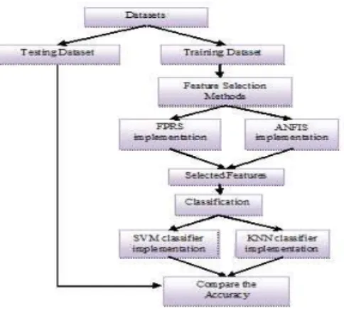
System Architecture:
Description of dataset:
The proposed work has been evaluated by experiments on various microarray data from UCI repository (UCI machine learning repository). The four datasets used to test the NFR method. The following table shows the summary of the microarray datasets.
Table 2: Summary of The Microarray Datasets.
Sl.No Dataset No. of Classes No. of Samples No. of Features
1 Leukemia 2 72 7129
2 Prostate 2 136 12600
3 Colon 2 62 2000
4 Breast 2 97 24481
Result And Findings:
The set of experiments designed to evaluate the performance of the NFR method by comparing the results among the kNN and SVM. The feature subset selection and classification processes have been shown in the following Fig 1, 2, 3 and 4 and the performance of our proposed work has been explained in Fig 5and 6. Similarly, Figure 7 and 8 show measure of number of features selected between NFR and existing feature selection methods and the accuracy of the NFR method.
In our work, we find that the important genes met our goal to diagnose the cancer. It helps to predict the cancer disease easily and give quick treatment.
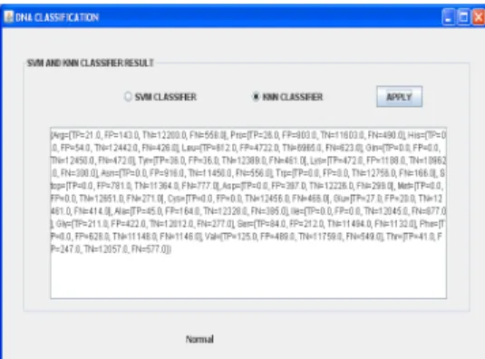
After feature subset selection, it is applied into KNN and SVM for Classification is defined by this Fig 2 and 3,
The comparison results are shown in fig7 and fig8,
Fig. 1: Feature selection.
Fig. 2: Selected Feature Subset.
Fig. 3: Selected features are applied into SVM Classifier for Classification.
Fig. 5: Accuracy Result for SVM Classifier.
Fig. 6: Accuracy Result for kNN Classifier.
Fig. 7: Comparison for accuracies of FPRS, ANFIS and FPRS+ANFIS with SVM Classier.
Conclusion And Future Work:
To conclude, a modest attempt has been made in this paper we analyzed the microarray data sets’ issues (to select the corrective set of genes and curse of dimensionality), by using the wrapper method of Neuro-fuzzy based feature selection technique. We also focused the FPRS and ANFIS for removing noise from the datasets. Then, this NFR hybrid feature selection method generated the feature subset with salient features. Finally, it’s applied in the classification algorithms (KNN and SVM) for evaluating the existing with the new one of the feature selection methods. Finally, obtained salient genes are evaluated with two classification algorithms (kNN and SVM).
In our future work, we may concentrate an in-depth study of multiclass cancer classification in an effective way.
REFERENCES
Cristianini, N. and J. Shawe-Taylor, 2000. “An introduction to Suport Vector Machines and other kernel-based learning methods”, Cambridge University press.
Farzana Kabir Ahmad, Dr. Safaai Deris, Dr. Norita Md. Norwawi, Dr. Nor Hayati Othman, 2008. “A Review of Feature Selection Techniques via Gene Expression Profiles”, IEEE.
Ghosh, A.K., 2006. “On optimum choice of k in nearest neighbor classification”, Computational Statistics & Data Analysis, 50: 3113–3123.
Gianluca Bontempi, 2007. “A Blocking Strategy to Improve Gene Selection for Classification of Gene Expression Data”, IEEE/ACM transactions on computational biology and bioinformatics, 4-2.
Gregory Piatetsky-Shapiro and Pablo Tamayo, “Microarray Data Mining: Facing the Challenges”, SIGKDD Explorations, 5: 2-1.
Guyon, I., J. Weston, S. Barnhill, V. Vapnik, 2002. “Gene selection for cancer classification using support vector machines,” Mach. Learn., 46(1–3): 389–422.
Jang, J.S.R., C.T. Sun, 1995. “Neuro-fuzzy modeling and control”, Proceedings of the IEEE, 83(3): 378– 406.
Jiawei Han and Micheline Kamber, 2006. “Data Mining Concepts and Techniques”, Second Edition. Jyh-Shing Roger Jang, 1993. “ANFIS: Adaptive-Network Based Fuzzy Inference System”, IEEE Transaction on system, Man, and Cybernetics, 23-3.
Martin Sewell, 2007. “Feature Selection”, <http://www.machine-learning.martinsewell.com/feature-selection/feature-selection/>.
Motoda, Hiroshi and Liu Huan, 2008. “Computational methods of Feature Selection”, Chapman & Hall/CRC Taylor & Francis Group, LLC. New York.
Qinghua Hu, Daren Yu, and Maozu Guo, 2010. “Fuzzy preference based rough sets”, Information Sciences, 180: 2003–2022, Elsevier Inc.
Sina Mahmoudi, Biyuk Sadeghi Lahijan, Hamidreza Rashidy Kanan, 2013. “ANFIS-Based Wrapper Model Gene Selection for Cancer Classification on Microarray Gene Expression Data”, 13th Iranian Conference on Fuzzy Systems (IFSC), IEEE.
UCI machine learning repository, <http://www.archive.ics.uci.edu/ml/>.
Ujjwal Maulik, 2014.“Fuzzy Preference based Feature Selection and Semi supervised SVM for Cancer Classification”, IEEE transactions on nanobioscience, 13-2.
Vapnik, V.N., 1998. ”Statistical Learning Theory”, Wiley.
Wang, Y., I.V. Tetko, M.A. Hall, E. Frank, A. Facius, K.F.X. Mayer, H.W. Mewes, 2005. “Gene selection from microarray data for cancer classification—a machine learning approach”, Computational Biology and Chemistry, 29: 37–46.
Witten, I.H., E. Frank, 1999.” Data Mining: Practical Machine Learning Tools and Techniques with Java Implementations”. Morgan Kaufmann.
Yvan Saeys1, Inaki Inza and Pedro Larranaga, 2007. “A review of feature selection techniques in bioinformatics”, Bioinformatics, Published by Oxford University Press, 23(19): 2507–2517.