A New Localization Algorithm
for Underwater Acoustic Sensor Networks
1
Farzaneh Famoori,
2Reza Javidan
1
Department of Computer Engineering, Arak Branch, Islamic Azad University
2
Department of Computer Engineering, Beyza Branch, Islamic Azad University
Abstract: Localization is one of most important technologies in Underwater Wireless Sensor Networks (UWSNs) since it plays a critical role in many applications. The variable speed of sound and the long propagation delays under water in addition to bandwidth limitations all pose a unique set of challenges for localization in UWSN. Localization algorithms are divided under two subcategories: range-based and range-free schemes. Range-based scheme uses measure distances or angles for estimating position of unknown node. But Range-free scheme uses stage-count or area-based schemes to estimate position of unknown node and does not need additional hardware. Range-free scheme is less accurate. On the other hand, range-based localization algorithms are not suitable for underwater networks because it needs additional hardware and also it does not act well. In this paper an improved range-free localization method is introduced. First ASP schema is simulated that is a range-free schema. Its drawback is to be less accurate due to its accuracy depends on distance determination. After that an improved method is presented that is based on range-free schema. In the proposed method, average distance between sensor node and connected anchor nodes, position of anchor nodes are given to a neural network. This neural network determinates position of sensor nodes after training. Simulation results in two distributed and centralized techniques are shown that improved algorithm includes high accuracy, fast convergence, wide coverage, low communication costs and good scalability features.
Key words: underwater Acoustic Sensor Network, localization, Range-based, Range-free, ASP algorithm, distributed technique, centralized technique.
INTRODUCTION
A vast portion of the earth surface is covered by water. Underwater Acoustic Sensor Networks are designed for activities such as gathering data related to ocean logy, pollution control, coastal explorations, avoiding disasters and stratagem and seafaring actions. The wireless underwater sensor networks emergence is a new opportunity for oceanic explorations (Akyildiz et al.,2005).
One of the major challenges in underwater localization networks is positioning the node. Localization is vital in applications such as positioning the accident point, helping submarine armada, avoiding disasters and so on. Localization, though in wireless sensor networks on earth is highly matured, still is a challenge in underwater networks as a result of inappropriate function of radio waves under water. And communications under water are through sound waves; hence GPS is not available underwater. In underwater networks positioning the nodes are necessary for a perfect and complete interpretation of the data such as the exact position of an event like a tsunami. Almost all the localization methods need to know the position of some nodes whose positions are determined by nodes called anchor nodes (Han et al., 2012).
Localization algorithms are divided into two: range-based and range-free. Range-based localization methods use techniques such as AOA, TDOA, TOA and RSS which need either the angel or distance and also synchronization among the transmitter and the receiver clocks. A simple method to synchronize is to use the time difference between the two miscellaneous signal entrances; the two signals having different flux speed are released at the same time. But in underwater networks, it is not possible to use radio signals. Flux delay is an important factor in synchronizing time in underwater networks algorithms and localization accuracy depends on the accuracy of the TOA or TDOA methods used. Algorithms using AOA method need the anchor and sensor nodes to be mobilized by special antennas. Also these algorithms make solving complicated nonlinear equations necessary which is not advantageous. Algorithms using RSSI for localization are influenced by multi path due to water surface reflection, water bed reflection and dispersion; hence, do not function perfectly (Chandrasekhar et al.,2012) (PC- Etter, 2003) (Chandrasekhar and Seah, 2006).
example, in geographical routing protocols or tracing the small water creatures (Chandrasekhar et al.,2012) (Bian et al.,2009 ) (Chandrasekhar and Seah, 2006).
Regarding what has been mentioned above, range-based methods do not function well under water. This research aims to introduce an optimized and intellectual algorithm based on the range-free method and to solve the range-free method problem which is inaccuracy and to optimize the localization accuracy. As it has been said before, in range-free method, two methods are used for distance recognition: area based and hop-count. Here a method is used which is a combination of algorithm ASP and overlapping connectivity. This method will be simulated and implemented by neural network.
The remainder of the article is organized as follows. In next Section the ASP algorithm is explained which is from range-free algorithms category. Then, the improved method is described in next section. After that the simulation results are explained. Finally the conclusion and remarks are outlined in end section. Many studies have been done in localization in underwater sensor networks. In this paper, two papers (Merrett and Tan, 2010) and (Yu et al.,2008) are used.
Ad Hoc Positioning System (Asp) Algorithm:
ASP is an example of a distributed connectivity-based localization algorithm that estimates node locations with the support of at least three anchor nodes, where localization errors can be reduced by increasing the number of anchors. Each anchor node propagates its location to all other nodes in the network using the concept of distance vector (DV) exchange, where nodes in a network periodically exchange their routing tables with their one-hop neighbours. Each node maintains a table {Xi, Yi, hi}, where {Xi, Yi } is the location of node iand hi is the distance in hops between this node and node i. When an anchor obtains distances to other anchors, it then determines an average size for one hop (called the correction factor), which too is then propagated throughout the network. The correction factor ci of anchor i is determined as:
(1)
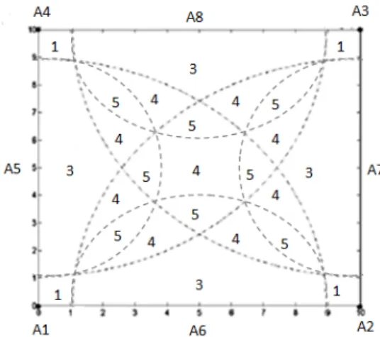
For all landmarks j ( ). Given the locations of the anchors and the correction factor, a node is then able to perform trilateration to estimate its own location. Figure 1 presents an example with three anchor nodes A1, A2, andA3. Anchor A1, knowing its Euclidean distances (50m and 110 m) and hop distances (two hops and six hops) to the other two anchor nodes, computes a correction of (50 + 110)/(2 + 6) = 20, which represents the estimated distance of a hop in meters. In a similar fashion, A2 computes a correction factor of 18.6 and A3 computes a correction factor of 17.3. Corrections are propagated via controlled flooding (i.e., once a node receives a correction, it ignores subsequent ones) to ensure that each node will only use one correction factor, typically from the closest anchor. For example, sensor node S in Figure 1 uses the correction factor obtained fromA2, that is, 18.6, to estimate its distances to the three anchors by multiplying the correction factor with the hop counts (leading to distances 3 × 18.6 to A1, 2 × 18.6 to A2, and 3 × 18.6 to A3). Given these distances, triangulation can be used to determine the position of S (Dargie and Poellabauer, 2010).
Fig. 1: Example of ASP localization.
• Problems of ASP Algorithm:
As previously it was said, Range-based localization methods do not function perfectly in underwater and range-free localization methods are more suitable in underwater. But range-free localization methods accuracy in comparison to Range-based localization methods is lower. These methods do not need any extra hardware and regarding the expenses are much more profitable than the range-based methods and energy usage is lower.
The problem with ASP method is that since the distance between sensor nodes and anchor nodes are presented as average distance, the estimated peculiarities are not accurate. And also it is possible that the sensor node is not placed at the intersection of all circles, hence the peculiarities achieved are not accurate and the error level is high.
should be fast so that it reports the actual location when data is sensed, wide coverage, low communication costs and good scalability features.
The Proposed Method:
Generally, we think of localization as an issue and by creating a neural network from all the received data from anchor nodes, a general map of the node position is estimated. This method uses neural network for achieving the real position of the node. In this section first the neural network is explained and then the improved method is presented.
• Neural Network Definition:
Neural networks are composed of simple elements which act parallel. These elements are inspired by biological neural systems. In nature, neural networks function is defined by the way they are connected. As a result, we can create an artificial structure subordinated to natural networks and by adjusting the amount of each connection under the title connection weight, determine the way its elements are related. After adjusting or neural network education, applied to a particular input leads to a particular response is received. The network will be compatible to accordance and hegemony of input and aim, until the network output and the aim output overlap. The composing elements of the network include neurons, transfer functions and layers. A neuron or some neurons next to each other form a layer. A network can be composed of either one or multiple layers. This network has an entrance layer which is not linear and an exit layer which is linear. In the entrance layer each neuron receives a single signal. This layer’s neurons only do the entering signal transfer action to the next layer which is a hidden layer. The network can have either one or multiple hidden layers which include neurons performing the main function. Each entering signal is passed to each neuron of this layer and the output of each neuron in this layer is transferred to neurons in the final layer which is the exit layer. The exit layer is responsible for the last phase of processing and sends out the outgoing signals. This network is called forward network since the data from incoming to outgoing are pushed forward. In this article the back propagation model of this network is used (fausett, 1994) (Coppin, 2006 ) (Kia, 1390).
• Overlapping Connectivity method:
In this way each node obtains its location as regards in common areas have been covered multiple node reference. References send their transition specification to periodic which can also include their location coordinates. Each node with receiving these signals of references determines that is located at the intersection of which node reference. And by taking the arithmetic mean of their distances to the node references, estimates its position (Bulusu et al.,2000).
• Improved Method Description:
The network structure in the improved method is as following:
-
This network includes eight anchor nodes. These anchor nodes are of DNA kind which is placed first above the water and after receiving their own peculiarities from GPS and updating they merge into water. And after a period under the water come to surface once again and this operation is repeated. In order to increase the DNA velocity, a DET is used which can increase and reduce the velocity.-
Nodes are stable in this network.-
This method does the fiscal operation of positioning in distributed and centralized manners.-
Different distance counting methods such as AOA, TDOA, RSS are available which do not function accurately under water. Hence, in order to achieve the distance, the average step (scale) is used.-
This method divides the network area into multiple areas (Merret and Tan, 2010). In order to do this, the overlapping connectivity method is used, according to which each 8 anchor nodes can send data up to a defined range. Nodes 1, 2, 3 and 4 are placed in the corners of the area which send data up to a specific range (90 meters) and nodes 5, 6, 7 and 8 are placed on the edge of the network also send data up to a specific range (40 meters). According to this a frame is achieved which looks like figure 2:Fig. 2: The achieved area regarding the sending range of reference nodes A1 to A8.
Each sensor node obtains its own position as following:
• Positioning the neighbor anchor nodes. Here the overlapping connectivity method is used in order to position the connected anchor nodes. Regarding the area the anchor nod is placed in the number of the connected anchor nodes is determined.
• Selecting anchor nodes positions and calculating the average step length. In order to determine the average step length, ASP method is used which is as following:
-
First, each anchor node calculates its distance with the neighbor anchor nodes through the steps connected between them and also calculated the number of the steps.-
Then, each anchor node calculates its own correction factor through the following formula and sends to the other nodes in the network.--
Each sensor node uses the anchor node’s correction factor which has the shortest step from it. Hence, it can achieve its distance from the anchor nodes by multiplying the correction factor into number of the steps.• Having the position of anchor nodes and the achieved average distance, a node can calculate its own exact position using the neural network. Calculating the real position of the sensor node by NN according to average step length which has been calculated in the last phase is as following:
In which K is the number of neural network inputs and D is the resultant which include the sensor node’s average step length to connected anchor nodes and the anchor nodes position. Shows the accurate calculated position of the sensor node and NN is the same neural network. Here, average step length between the sensor node and the connected anchor nodes and the connected anchor nodes position is presented as an input to a neural network.
Regarding the area the node is placed in another calculation is done. Figure 3 shows the neural network structure. For example if the sensor node is placed in area 3, NN3 is used.
Simulation Results:
• Simulation adjustments:
Stimulation takes place in Matlab environment. In this simulation the area is 100*100 meters and 8 anchor nodes are placed in each corner and edges. Each anchor node which is placed in a corner of the area can send sound signals up to the range 90 meters. And each node placed on the edges of the area can send sound signals up to the range 40meters. And this simulation takes place in shallow water.
Then 30 sensor nodes are distributed accidentally in this area. Figure 4 shows the network area.
Fig. 4: Sensor nodes distribution for stimulation
In order to evaluate the improved and the main methods two following parameters are used:
1. Localization error: the difference between the estimated position and the real position X from the node which is calculated through the following formula:
(5)
2. Average localization error: the average difference between the estimated position and the real position from all nodes which is calculated through the following formula:
(6)
• Results of simulation:
In this section simulation ASP algorithm and the improved method are applied in Matlab environment. In order to stimulate the improved method, this method is implemented through neural network. In order to train the neural network the back propagation network is used and the education dependent is Trainrp. The input and hidden layer function is Logsig and the output layer function is Pureline function. Figure 5, 6 and 7 in order of appearance show the result of the ASP method simulation and the method.
Concusions:
In this article, an intellectual range-free localization method is introduced for sound sensor networks under water. In the improved method, the sensor nodes do not need extra hardware in order to achieve the distance or data such as AOA, TOA, RSS. The sensor nodes can achieve their position through the resulted average step and the connected anchor nodes. A neural network plays a main role in the improved method. In this method localization in considered as an issue and by neural network the accurate position of the sensor node is achieved. The method is stimulated in Matlab environment. During the simulation it was clarified that the improved method has a much better function than the available method ASP and decreases the localization error in a considerable manner and raises the accuracy of localization. Simulation results in two distributed and centralized techniques are shown that improved algorithm include high accuracy, fast convergence therefore, since nodes may drift due to water currents, the localization procedure should be fast so that it reports the actual location when data is sensed, wide coverage, low communication costs and good scalability features because all the network nodes are localized.
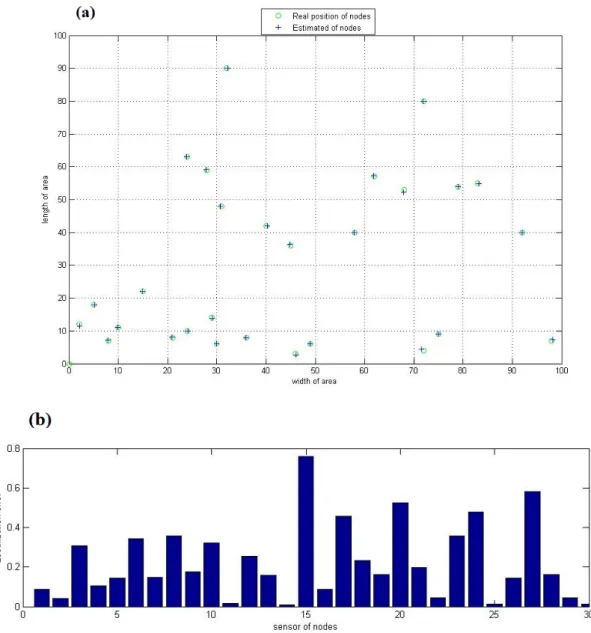
Fig. 6: Result of simulation of the improved method by NN in centralized localization: (a) result of location estimation; (b) error result.
Table 1: The simulation results of ASP method and the improved method
Maximum error Minimum error
Average error
60 0.1
9.1 ASP method
0.7 0.008
0.3 improved method in centralized localization
0.14 0.01
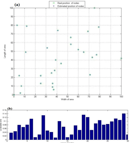
Fig. 7: Result of simulation of the improved method by NN in distributed localization: (a) result of location estimation; (b) error result.
REFERENCES
Akyildiz, IF., D. Pompili, T. Melodia, 2005. Underwater acoustic sensor networks: research challenges. Ad Hoc Networks 3, Elsevier.
Han, G., J. Jiang, L. Shu, Y. Xu and F. Wang, 2012. Localization Algorithms of Underwater Wireless Sensor Networks: A Survey. Sensors, no. 2: 2026-2061.
Chandrasekhar, V., W. KG Seah, Y. Choo, H. Voon Ee, 2006. Localization in Underwater Sensor Networks :Survey and Challenges. WUWNet’06, September 25, 2006, Los Angeles, California, USA.
Etter, P.C., 2003. Underwater Acoustic Modeling and Simulation. 3rd Edition, Spon Press, New York, 2003. Bian, T., R.Venkatesan, and C. Li, 2009. Design and Evaluation of a New Localization Scheme for Underwater Acoustic Sensor Networks. in Global Telecommunications Conference, GLOBECOM, Nov. 30 2009.
Chandrasekhar, V. and W.K.G. Seah, 2006. Area Localization Scheme for Underwater Sensor Networks. Proc. IEEE OCEANS Asia Pacific Conf., pp: 1-8.
Merrett, G.V. and Y.K. Tan, 2010. Wireless Sensor Networks: Application - Centric Design. ISBN 978-953-307-321-7, Published: December 14, 2010, chapter 17.
Yu, S., J. Lee, W. chung, E. kim, S. kim, 2008. A soft computing approach to localization in wireless sensor networks. elsevier Ltd.
Dargie, W., C. Poellabauer, 2010. Fundamentals of Wireless Sensor Networks, Theory and Practice. copyright 2010 John Wiley & Sons Ltd, ISBN: 978-0-470-99765-9.
Hereman, W. Trilateration, The Mathematics Behind a Local Positioning System. PDF fausett, L., 1994.Fundamentals of Neural Networks: Arquitectures, Algorithms, and Application. ISBN 8131700534, 9788131700532.
Coppin, B., 2006. Artificial Intelligence Illuminated. ISBN 0-7637-3230-3, 2004, publisher Pearson Education,