Vorren_unc_0153D_17010.pdf

A DIRECT SEARCH FOR DARK MATTER WITH THE MAJORANA DEMONSTRATOR

Kristopher Reidar Vorren

A dissertation submitted to the faculty at the University of North Carolina at Chapel Hill in partial fulfillment of the requirements for the degree of Doctor of Philosophy in the

Department of Physics.

Chapel Hill 2017

c 2017

ABSTRACT

Kristopher Reidar Vorren: A Direct Search for Dark Matter with the Majorana Demonstrator

(Under the direction of Reyco Henning)

ACKNOWLEDGEMENTS

The work presented here was only possible because of the support provided by so many people over the last several years. My gratitude is not limited to those specifically acknowl-edged here–there are simply too many people that deserve thanks.

I want to first thank everyone on the Majoranacollaboration. Despite the great stress that comes along with doing good science, the collaboration stayed focused and achieved significant milestones over the last several years. It has been a great pleasure to work with everyone involved, even when that work took place in a cleanroom, one mile underground. This dissertation would never have been written without the overwhelming support from my collaborators.

I am grateful to have been a part of the UNC community and especially the Experimen-tal Nuclear and Astroparticle Physics (ENAP) group. Special thanks goes to my advisor, Reyco Henning, who helped me navigate my way through the unending obstacles that arose throughout graduate school. I have to thank John Wilkerson who always seemed to ask the tough questions that ultimately kept me on course for graduation. The other students and the postdocs that have come and gone also deserve thanks; their support and advice was extremely helpful.

here to read this.

TABLE OF CONTENTS

LIST OF TABLES . . . x

LIST OF FIGURES . . . xi

LIST OF ABBREVIATIONS AND SYMBOLS . . . xiv

1 Introduction . . . 1

1.1 The Case for Dark Matter . . . 1

1.1.1 Indirect Observational Evidence . . . 3

1.1.2 Cosmological Models with Dark Matter . . . 10

1.2 Particle Dark Matter Candidates . . . 14

1.2.1 Weakly Interacting Massive Particles . . . 15

1.2.2 Axions . . . 17

1.2.3 Bosonic keV-Scale Dark Matter . . . 22

1.3 Outline of Dissertation . . . 25

2 Semiconductor Detectors and the P-type Point-Contact Germanium De-tector . . . 26

2.1 Properties of Semiconductor Detectors . . . 26

2.1.1 Introduction . . . 26

2.1.2 The Band Gap Model . . . 27

2.1.4 Semiconductor Junction . . . 30

2.2 High Purity Germanium Detectors . . . 32

2.2.1 Crystal Fabrication . . . 33

2.2.2 Conventional Ge Detector Configurations . . . 35

2.3 PPC Detectors . . . 36

2.3.1 Noise Characteristics . . . 36

2.3.2 Detector Resolution . . . 41

2.3.3 Charge Collection in PPC Detectors . . . 43

2.3.4 Slow Pulses . . . 45

2.4 Summary and Discussion . . . 47

3 The Majorana Demonstrator . . . 48

3.1 Experiment Overview . . . 48

3.1.1 Neutrinoless Double-Beta Decay . . . 48

3.1.2 Experiment Goals . . . 51

3.2 Experiment Infrastructure and Hardware . . . 56

3.2.1 The Majorana Lab Infrastructure . . . 56

3.2.2 Detector, String, and Cryostat Assembly . . . 59

3.2.3 Detector Shielding . . . 62

3.3 Module 1 . . . 63

3.3.1 Configuration . . . 64

3.3.2 Electronics Readout and Performance . . . 66

3.3.4 Anticipated backgrounds . . . 69

4 Characterization of Data and Systematics . . . 71

4.1 Data Selection . . . 71

4.1.1 Data Description . . . 71

4.1.2 Analysis Live-time and Exposure Determination . . . 72

4.2 Low-Energy Calibration . . . 76

4.2.1 MJD Energy-Scale Calibration . . . 76

4.2.2 Correcting the Low-Energy Calibration . . . 78

4.2.3 The DS0 Low-Energy Spectrum . . . 83

4.3 Resolution Measurement . . . 83

4.3.1 Fitting the Resolution below 100 keV . . . 84

4.3.2 Resolution Fit Parameters . . . 86

4.4 Summary of Systematic Parameters . . . 86

5 Data Cleaning . . . 88

5.1 Surface Event Removal . . . 88

5.1.1 The T /E parameter . . . 88

5.2 Electronic Noise Removal . . . 92

5.2.1 Tagging and Removing Pulser-Retriggering Events . . . 92

5.2.2 Transient Pulse Identification and Removal . . . 95

5.3 Data Cleaning Efficiency . . . 98

5.3.1 Acceptance Efficiency of the Multiplicity Cut . . . 98

5.3.3 The T /E-Cut Acceptance Efficiency . . . 100

5.4 Data Cleaning Summary . . . 104

6 Profile Likelihood Analysis and Results . . . 106

6.1 The Profile Likelihood Method . . . 106

6.1.1 Constructing the Profile Likelihood Function . . . 107

6.1.2 Building the Signal and Background Model . . . 110

6.2 Results . . . 114

6.2.1 Search for keV-scale bosonic pseudoscalar DM . . . 115

6.2.2 Vector bosonic dark matter results . . . 119

6.2.3 Solar axions produced in the57FeM1 transition . . . 120

6.2.4 Pauli Exclusion Violating Decay . . . 123

6.2.5 Electron Decay . . . 126

7 Conclusion . . . 127

7.1 Overview . . . 127

7.2 Outlook . . . 128

LIST OF TABLES

1.1 Parameters from the CMB . . . 14

3.1 List of select double-beta decaying isotopes . . . 51

4.1 Detectors’ Active Mass . . . 76

4.2 Cosmogenic Background Isotopes . . . 79

4.3 Low-Energy 228Th Peaks . . . 83

4.4 Systematic Parameters . . . 87

5.1 Data Cleaning Parameters . . . 105

6.1 Likelihood Analysis Parameters . . . 115

LIST OF FIGURES

1.1 Doppler shift in NGC 7531 . . . 6

1.2 Rotation Curve of NGC 6503 . . . 7

1.3 The Bullet Cluster . . . 9

1.4 Anisotropy in the CMB . . . 12

1.5 CMB Power Spectrum . . . 13

1.6 Predicted WIMP ionization spectrum . . . 17

1.7 WIMP exclusion plot . . . 18

1.8 Light shining through wall experiment . . . 21

1.9 Constraints on vector dark matter . . . 23

2.1 Band Gap Model in Solids . . . 28

2.2 Semiconductor Impurities . . . 30

2.3 Semiconductor Junction Physics . . . 31

2.4 Germanium zone refinement . . . 33

2.5 Simplified Czochralski process . . . 34

2.6 Germanium Detector Configurations . . . 37

2.7 Noise curve and components . . . 39

2.8 Detector Drift paths . . . 44

2.9 PPC Weighting Potential . . . 45

2.10 PPC Pulse Timing . . . 46

3.1 Overview of the Majorana Demonstrator . . . 49

3.2 A=76 Decay Scheme . . . 50

3.3 2νββ and 0νββ . . . 52

3.4 0νββ sensitivity limit . . . 53

3.5 0νββ discovery potential . . . 54

3.7 Majorana Lab Space . . . 58

3.8 Detector and String Assemblies . . . 60

3.9 MJD Shield Outline . . . 63

3.10 Module 1 orientation . . . 64

3.11 Module 1 . . . 65

3.12 Detector readout electronics . . . 66

3.13 Module 1 DAQ Overview . . . 68

3.14 Background rate in 0νββ ROI . . . 69

4.1 Operable Detectors . . . 73

4.2 Run vs Energy . . . 74

4.3 228Th calibration spectrum . . . 79

4.4 Detector Energy Offset Errors . . . 80

4.5 Natural Detector Spectrum (corrected offset) . . . 81

4.6 Attenuated vs Unattenuated Energy . . . 82

4.7 Calibrated Low-Energy Spectra . . . 84

4.8 Resolution Fit Function . . . 85

5.1 Effect of the triangle filter . . . 90

5.2 Triangle Filtered Waveforms . . . 90

5.3 T/E vs E . . . 91

5.4 Examples of Electronic Noise . . . 92

5.5 Comparison of Tail Minimum Parameters . . . 93

5.6 Comparison of Tail Minimum Parameters . . . 94

5.7 Transient Event Tagging with Waveform Minima . . . 96

5.8 The T /E vs E parameter with electronic noise removed. . . 97

5.9 Tail min cut rejection . . . 100

5.11 PulserT /E Tuning . . . 102

5.12 T /E acceptance curves . . . 103

6.1 Profile Curve for a 14.4 keV peak signal . . . 109

6.2 Germanium Photoelectric Absorption Cross Section . . . 117

6.3 Axio-Electric coupling upper limit (90% confidence limit) . . . 118

6.4 Vector-Electric coupling upper limit (90% confidence limit) . . . 120

6.5 Solar axion coupling limit . . . 122

6.6 Model best fit for 14.4 keV solar axion signal . . . 122

LIST OF ABBREVIATIONS AND SYMBOLS

0νββ Neutrinoless Double-beta Decay 2νββ Double-beta Decay

BEGe Broad Energy Germanium C.I. Confidence Interval

CMB Cosmic Microwave Background

DFSZ Dine, Fischler, Srednicki, and Zhitnitsky Axion Model DM Dark Matter

GAT Germanium Analysis Toolkit HPGe High Purity Germanium

KSVZ Kim, Shifman, Vainstein, and Zakharov Axion Model PDF Probability Distribution Function

PEP Pauli Exclusion Principle PPC P-type Point Contact

Q End-point Energy ROI Region of Interest SBC Single Board Computer

SURF Sanford Underground Research Laboratory WIMP Weakly Interacting Massive Particle

CHAPTER 1: Introduction

Roughly 80% of the matter density in the universe is hypothesized to be non-baryonic ‘dark matter.’ While the evidence for dark matter is well-established, it’s based upon indirect observation resulting from its gravitational interactions. The exact nature of dark matter remains unknown, though cosmologists tend to favor a cold, exotic, non-Standard Model particle as the dominant dark matter candidate. A direct discovery via a particle interaction would confirm its identity as a new type of particle and help elucidate its fuller complexion. Several experiments are currently attempting to directly detect dark matter interactions. This dissertation focuses on direct dark matter detection efforts with the Majorana De-monstrator.

Section 1.1: The Case for Dark Matter

The concept of dark matter is neither neither new nor astounding. In its earliest usage, ‘dark matter’ referred to any mass whose existence had been inferred, yet remained unde-tected by (traditionally optical) observation or experimentation. Examples included cold, non-luminous objects such as dead stars, planets, or clouds of gas. Towards the latter half of the 20th century–as the field of astroparticle physics emerged–the term dark matter became more synonymous with exotic, extra-Standard Model mass. Since then, direct detection of particle dark matter has become an active field of research and the main focus of multi-ple experiments. While the constitution of dark matter is the subject of much debate, it’s existence is well-established by virtue of the multitude of indirect evidence.

of gravitationally anomalous motion often provided clues of unobserved objects, leading to important discoveries in astrophysics. Notable examples include the discovery of a compan-ion star orbiting Sirius (known as ‘Sirius B’) and the discovery of Neptune [1]. Almost two decades before Alvan Graham Clark first observed Sirius B, Friedrich Bessel deduced its presence based on its irregular motion, claiming that such motion would not be surprising if it were a double star system [2]. Similarly, John Galle first observed Neptune after Urbain Le Verrier precisely predicted its location based on observations of Uranus [3]. Historical examples like these coupled with modern observations of anomalous motion of galactic and larger scale structures motivate searches for dark matter.

To avoid being disingenuous, another case of unusual motion worthy of cognizance is the anomalous precession of Mercury’s perihelion, with discovery credited to Le Verrier. The perihelion precesses roughly 43 arcseconds/century faster than predicted by Newtonian gravitational dynamics. The fast precession led astronomers to believe that a hypothetical protoplanet, named Vulcan, was perturbing the orbit. Numerous claims of the observation of Vulcan were made throughout the latter half of the 19thcentury. With each claim, Le Verrier would attempt to correct Vulcan’s orbital parameters to predict its next transit by the sun. Many in the astronomy community at the time doubted Vulcan’s existence after Le Verrier’s calculations did not correctly predict further sightings. The resolution to this conundrum had to wait until 1915 when Albert Einstein demonstrated that Mercury’s precession could be explained within the framework of General Relativity.

the scope of this dissertation.

The case for dark matter is built from indirect observational evidence and successful integration into the standard cosmological framework, i.e ΛCDM. Some well-known examples that lend credence to the dark matter hypothesis include:

• Unaccounted mass found via virial theorem audit

• Galaxy mass distributions inconsistent with rotational curves • Gravitational lensing of distant galactic clusters

• X-ray observation of hot gas within clusters • Cosmic microwave background anisotropy

• Deuterium abundance via primordial nucleosynthesis Further discussion expanding on these considerations follows.

1.1.1: Indirect Observational Evidence

By the end of the 19th century, searches for dark objects within the Milky Way were underway. Dynamical models were used as a tool to set upper limits on the amount of dark matter within the galaxy. Lord Kelvin conceptualized a uniformly dense gaseous model of stars in the galaxy with gravity acting as the inter-particle force mediator. Using variations of this model, Kelvin, Henri Poincar´e, Ernst ¨Opik, Jacobus Kapteyn, and Jan Oort were able to estimate the total mass within the solar neighborhood, i.e. within roughly 3000 light years of the sun [1, 5–8]. Noting that the predicted velocity dispersion is similar to that of the observed matter, they concluded that the density of non-luminous matter within the neighborhood cannot exceed the luminous density.

Virial Theorem

analysis of galaxy cluster observations made by Edwin Hubble and Milton Humason [9]. A galaxy cluster is large scale structure consisting of hundreds or thousands of galaxies that are gravitationally bound. The majority of baryonic mass in galaxy clusters is found in the intra-cluster medium, consisting of extremely hot, O(106 _{K), gas. Zwicky particularly}

focused on the Coma cluster, noticing that galaxies within it exhibited large differences in velocity, upwards of 2000 km/s. With the measured velocity dispersions, he was able to apply the virial theorem to estimate the total mass of the cluster [10, 11].

The virial theorem provides an expression for the time averaged kinetic energy of a system of particles (entire galaxies in this case). If the intra-particle potential is of the form

V(r) = arn, then the virial theorem can be stated as,

hTi=nhVtoti (1.1)

where T is kinetic energy, Vtot is the potential energy of the system, and h·i denotes time

averaging. Gravitation has a 1/r potential, son =−1. Inserting the gravitational potential yields the result,

σ2 ≈ GM

R (1.2)

whereσis the velocity dispersion,Gis the universal gravitation constant, andM is the mass within a spherical volume of radius R.

Zwicky estimated the total mass of the Coma cluster to be the product of the roughly 1000 observed galaxies and the average galactic mass, about 109 M. The radius was

characterization of the distribution of dark matter in the Coma cluster and other galaxy clusters is ongoing [12, 13].

Galactic Rotation Curves

Galactic rotation curves describe the average rotational velocity1 of visible objects as a function of distance from the galactic center. Typically, the center of a galaxy is its most luminous feature, motivating the conclusion that the central region encompasses a plurality of the galactic mass. From the density profile, it is possible to predict the rotational velocity of stars or gases in galaxies at varying distances. For many galaxies, the predicted rotation curves do not match the measured curves, particularly for large radii. Dark matter provides an explanation for the disparity amongst the measured and predicted galactic rotation curves. Using a spectrogram, the rotation of a galaxy is measured by analyzing the doppler shift along its major axis. If the galaxy is rotating, light from the arm approaching the observer will be blue shifted while light from the receding arm will be red shifted. A transition signa-ture would be noted at the galactic center. Figure 1.1 shows an example of the doppler shift for NGC 7531. Precursory spectrographic measurements of the Andromeda Galaxy (M31, NGC 224) taken in 1914 by Max Wolf and Vesto Slipher [1, 14] provided evidence of nebular rotation: a linear correlation between wavelength and position along the major axis was apparent.

Over the next few decades several additional rotational profiles for M31 were measured out to increasing distances as technology improved, e.g. [8, 16]. At the time, it was deter-mined that the mass-to-light ratio of Andromeda agreed well with the solar-neighborhood M/L ratio. In the late 1930s, Horace Babcock [17] measured increasing rotational veloci-ties up to distances of 1.5◦ from the galactic center, which suggests the existence of a large amount of mass at extreme distances. Extra mass affects the M/L ratio, but Babcock

ar-1_{For this discussion, the rotational velocity refers to the transverse orbital speed in dist/time, not the angular}

1987ApJS

...

64

....

IB

26 BUTA Vol. 64

Fig. 32.—Phases of the even Fourier terms with respect to the line of nodes in the galaxy plane, for both the B and the / passband

Fig. 33.—Emission-line rotation curve of NGC 7531. Note slight asymmetry between the northeast (negative radii) and southwest (positive radii) sides, and also how the inner ring lies very close to the “turnover radius” on each side. Points based on only a single spectrum are indicated by open circles.

Least-squares fits to the observed rotation curve were then made, allowing spheroid and disk to have different values of M/L. It was found that, for both passbands, best fits are obtained if the bulge either is ignored or has a much smaller M/L than the disk. In either case the light distribution provides a poor representation of the rotation curve. The inner ring causes a large effect even in the I band which is not

observed, while the inner regions predict too steep a rise and the outer regions predict a decline where the rotation velocity is mostly constant.

The decline in the outer parts is similar to that predicted by light distributions in NGC 753, NGC 1085, and NGC 2998 observed by Kent (1986), and suggests that NGC 7531 has a massive halo of dark matter. However, at least some of the

© American Astronomical Society • Provided by the NASA Astrophysics Data System Figure 1.1: Effect of doppler shifting on the measured velocities as a function of distance (measured in arcseconds). The red shifted arm at positive angles shows above average velocities, while the blue shifted arm on the left exhibits below average velocities. Figure from [15].

gued that the ratio was biased due to intra-galactic light absorption. By the mid 1950s, larger telescopes had been deployed as the field of radio astronomy was becoming more prominent. These telescopes were capable of observing the 21 cm hydrogen-one (Hi) line, facilitating an additional method of measuring galactic rotation curves that could probe very large distances. See for example, [18] and [19].

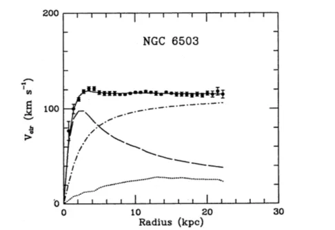
It wasn’t until the 1970s that astronomers were convinced that rotation curves were al-luding to the presence of large quantities of mass missing from galactic mass estimates. In 1970, Rubin and Ford [20] published their oft-cited paper that presented optical measure-ments of M31 rotation curves out to ∼ 2◦ of arc using an image-tube spectrograph. They noted similarities between their measured rotation curves and previous M31 curves obtained from Hi observations [18, 21]. It was the flattening of rotation curves far from the galactic center that was confounding to astronomers, see figures 1.1 and 1.2. By the late 1970s, many results from additional galaxies had been published with similar findings; see [1] and references therein.

Figure 1.2: Rotation curve of NGC 6503. The dotted, dashed, and dash-dotted lines are the contributions from gas, disk (visible), and dark matter respectively. Figure from [22].

mechanics if a constant M/L ratio for the considered galaxy is assumed. At large distances, the expected rotational velocity, v, as a function of radius is roughly given by,

v(r) =

r

GM(r)

r , (1.3)

whereM(r) is the total mass within a spherical radius randGis the universal gravitational constant. From luminosity profiles, the expectation for spiral galaxies such as M31 is that most of the mass resides at the center, and so Eqn. 1.3 would predict that the velocity should fall off asv ∝ r−1/2. Rubin and Ford attempted to correct for the large quantity of hydrogen far from the center of M31, but determined that the gas only accounted for 4-8% of the mass at large radii. The non-luminous mass required to explain the flat rotation curves lays the groundwork for the ‘missing mass problem.’

with density given by the Navarro-Frenk-White profile [23], envelopes the galaxy:

ρ(r) = ρ0 r Rs

1 + _Rr

s

2 . (1.4)

Here ρ0 is a normalization parameter, and Rs is a radial scale parameter that characterizes the halo. Note that evaluating the spherical volume integral to O(Rs) and dividing by the radius (as per equation 1.3) reproduces a dark matter velocity profile similar to the curve in figure 1.2. Navarro, Frenk, and White used n-body simulations to inspire the NFW profile, assuming a standard cold dark matter (CDM) cosmology. Section 1.1.2 will further discuss the ΛCDM model.

Gravitational Lensing & X-ray Observations of Galactic Clusters

Further evidence of dark matter can be inferred from gravitational lensing. General Relativity states that the presence of mass curves space-time [24], thereby altering the tra-jectory of nearby particles. This includes photons, meaning that nearby sources of mass can effectively refract light rays. Massive objects between an observer and a distant light source can thus produce a lensing effect. From the shear of the lensing field, it’s possible to extract the distribution of the lensing mass. The effect is usually weak and typically requires that several distant sources are analyzed to determine their preferred distortion direction, from which one can determine the direction to the center of the lens. The invisible dark matter in galaxy clusters can often produce strong lensing effects that enhance the apparent ellipticity of luminous galaxies. The total mass estimate from the gravitational lens can be compared with luminous mass estimates to provide a lower limit of the dark matter content. Typical clusters are comprised of roughly 80% dark matter and 20% baryonic matter. For a comprehensive review of DM gravitational lensing see [25].

Figure 1.3: Left: Color image from the Magellan images of the merging cluster 1E 0657-558. The white bar indicates 200 kpc at the distance of the cluster. Right: Chandra x-ray image of the colliding clusters. The green contours in both panels represent weak gravitational lensing reconstructions of the distribution of mass. Figure from [28].

the 10-100 MegaKelvin range. Hot gas accounts for between 50-90% of the baryonic mass in most clusters, with larger fractions found in the more massive clusters. As hydrogen is the most abundant element in the universe, the intra-cluster plasma consists of mostly protons and electrons, however trace amounts of helium and other heavier nuclei are found in minuscule abundance. The gravitational potential due to stars and galaxies within a cluster is not strong enough to bind the hot gas to the system. Dark matter is required to ensure that the gas does not disperse away from the cluster [26]. Kravtsov and Borgani provide a review of galaxy cluster formation in [27].

baryonic gas particles from both clusters caused turbulence during the collision, effectively impeding the bulk momenta of the gas. The distribution of matter in the bullet cluster can be used to constrain the self interaction of dark matter particles [29, 30].

1.1.2: Cosmological Models with Dark Matter

Dark matter can explain many artifacts in models stemming from big bang cosmol-ogy [31]. The standard model of cosmolcosmol-ogy is the ΛCDM paradigm because it’s the simplest model capable of accounting for observed cosmological phenomena. ΛCDM describes a uni-verse undergoing accelerated expansion, described by a cosmological constant (Λ), and cold dark matter (CDM) [32, 33]. The standard cosmological model explains observations such as the anisotropy in the cosmic microwave background (CMB), the abundance of light elements synthesized in the nascent universe, and the formation of large scale structures, i.e galaxy distribution (discussed more in section 1.2). A dark matter component is required in each of these examples to explain their observed features. Universal expansion requires dark energy (see for example [34]), which is not discussed here.

Cosmic Microwave Background

Primordial radiation in the microwave region of the electromagnetic spectrum can be detected from all directions in the sky [35]. The cosmic microwave background (CMB) radiation is the oldest in the universe, dating back to the period of recombination2 when the universe was roughly 380,000 years old. Prior to recombination, the temperature and the density of the early universe was much greater than it presently is. Baryonic matter existed in an opaque (blackbody) plasma state; Thompson scattering prevented photons from freely traveling through space. As the universe cooled, protons and electrons combined to form neutral atoms. The abundance of free charge in the universe dropped by many orders of

2_{The term recombination can be misleading since there were no neutral atoms prior to this epoch. The usage}

magnitude resulting in a transparent universe. This drop in the rate of photon scattering is called photon decoupling. Since decoupling, expansion of the universe (and thus photon wavelength) has cooled the CMB temperature to about 2.7 K. As the name implies, the relic CMB radiation now permeates the sky as an irreducible, highly isotropic microwave background.

Although the temperature of the CMB is mostly isotropic, well-documented O(10−5 _K)

thermal angular anisotropies have been measured. Since the accidental discovery of the CMB by radio astronomers Penzias and Wilson, increasingly advanced telescopes have sought to characterize the angular anisotropies. RELIKT-1 [36, 37], launched by the Soviet Union in 1983, was the first space based telescope to map the CMB. In 1989 the COBE [38, 39] satellite was launched by NASA. Both experiments reported their findings in 1992, confirming the blackbody frequency distribution and slight anisotropy of the background predicted by ΛCDM. Succeeding COBE was the WMAP [40] telescope, which provided improved angular resolution enabling the characterization of multiple peaks in the multipole power spectrum. WMAP was retired in 2010 after the launch of the current generation spacecraft, PLANCK [33, 41]. A map of the temperature anisotropy is shown in figure 1.4. The multipole power spectrum is also shown in figure 1.5.

Analyzing anisotropies in the CMB via the temperature power spectrum can help cos-mologists infer important parameters such as the curvature of the universe, the expansion rate of free space, the abundance of baryonic and dark matter, and the sum of the neutrino masses. The most current cosmological parameters are fit from the PLANCK CMB survey and a subset of the parameters is shown in table 1.1.

Figure 1.4: Map of the anisotropy in the cosmic microwave background. The CMB tem-perature is fairly uniform averaging 2.7260 K and varying by ∼600 µK. Figure from [42].

Space-time quantum fluctuations perturbed the plasma, generating acoustic oscillations. The peaks in the spectrum are the result of various phenomena: the location of the first peak in the multipole spectrum is impacted by space-time curvature, the second peak is evidence of plasma acoustics and gauges the abundance of baryonic matter. The prominence of the third peak, along with the dampening of peaks at higher multipoles, indicates the presence of non-baryonic dark (i.e electrically neutral) matter during recombination. For an accessible, qualitative overview of the CMB power spectrum by Wayne Hu, see [44].

Primordial Nucleosynthesis

The lightest metallic (i.e. not 1H) isotopes in the universe were produced during primor-dial, or big bang nucleosynthesis (BBN). The duration of this epoch covers∼10 s to∼1 hour after the big bang. The abundances of 2H, 3He, 4He, and 7Li are characterized by the ratio of baryons to photons. BBN is capable of explaining the large abundance of 4He in the universe, ∼25% of baryonic matter. While 4_{He is produced in stars, stellar production}

Planck Collaboration: Cosmological parameters 0 1000 2000 3000 4000 5000 6000 D TT [ µ K 2 ]

30 500 1000 1500 2000 2500

-60 -30 0 30 60 D TT 2 10 -600 -300 0 300 600

Fig. 1.Planck2015 temperature power spectrum. At multipoles` 30 we show the maximum likelihood frequency-averaged temperature spectrum computed from thePlikcross-half-mission likelihood, with foreground and other nuisance parameters de-termined from the MCMC analysis of the base⇤CDM cosmology. In the multipole range 2`29, we plot the power spectrum estimates from theCommandercomponent-separation algorithm, computed over 94 % of the sky. The best-fit base⇤CDM

theoreti-cal spectrum fitted to thePlanckTT+lowP likelihood is plotted in the upper panel. Residuals with respect to this model are shown

in the lower panel. The error bars show±1 uncertainties.

The large upward shift inAse2⌧reflects the change in the

abso-lute calibration of the HFI. As noted in Sect.2.3, the 2013 analy-sis did not propagate an error on thePlanckabsolute calibration through to cosmological parameters. Coincidentally, the changes to the absolute calibration compensate for the downward change in⌧and variations in the other cosmological parameters to keep the parameter 8largely unchanged from the 2013 value. This

will be important when we come to discuss possible tensions between the amplitude of the matter fluctuations at low redshift estimated from various astrophysical data sets and thePlanck

CMB values for the base⇤CDM cosmology (see Sect.5.6).

(4) Likelihoods. Constructing a high-multipole likelihood for

Planck, particularly withT E andEE spectra, is complicated and difficult to check at the sub- level against numerical

simulations because the simulations cannot model the fore-grounds, noise properties, and low-level data processing of the realPlanckdata to sufficiently high accuracy. Within the Planckcollaboration, we have tested the sensitivity of the re-sults to the likelihood methodology by developing several in-dependent analysis pipelines. Some of these are described in

Planck Collaboration XI(2016). The most highly developed of

them are theCamSpecand revisedPlikpipelines. For the 2015

Planckpapers, thePlikpipeline was chosen as the baseline. Column 6 of Table1lists the cosmological parameters for base

⇤CDM determined from the Plik cross-half-mission likeli-hood, together with the lowP likelilikeli-hood, applied to the 2015 full-mission data. The sky coverage used in this likelihood is identical to that used for theCamSpec2015F(CHM) likelihood. However, the two likelihoods di↵er in the modelling of

instru-mental noise, Galactic dust, treatment of relative calibrations, and multipole limits applied to each spectrum.

As summarized in column 8 of Table 1, the Plik and CamSpecparameters agree to within 0.2 , except forns, which

di↵ers by nearly 0.5 . The di↵erence innsis perhaps not

sur-prising, since this parameter is sensitive to small di↵erences in

the foreground modelling. Di↵erences innsbetweenPlikand

CamSpecare systematic and persist throughout the grid of ex-tended⇤CDM models discussed in Sect.6. We emphasize that

theCamSpecandPliklikelihoods have been written indepen-dently, though they are based on the same theoretical framework. None of the conclusions in this paper (including those based on the full “TT,TE,EE” likelihoods) would di↵er in any substantive

way had we chosen to use theCamSpeclikelihood in place of . The overall shifts of parameters between the 2015

Figure 1.5: The CMB temperature power spectrum (TT). The red curve shows the best-fit when incorporating parameters from the λCDM model. Residuals are shown in the bottom plot. Error bars cover ±1σ uncertainty. The parameter DT T

l =l(l+ 1)ClT T/2π, where ClT T is the expectation value of the spherical harmonic power coefficient as a function of l [43]. Figure from [33].

Table 1.1: A select list of parameters determined from the anisotropy in the CMB. Most recent values from [33].

Parameter Description Value Unc. Units

H0 Hubble Constant 67.8 0.9 km Mpc−1 s−1

h Reduced Hubble Const 0.678 0.009

Ωm Matter Density Parameter 0.308 0.012

Ωbh2 Baryonic Density 0.02226 0.00023

Ωch2 DM Density 0.1186 0.0020

|Ωk| Curvature Parameter <0.005

Σmν Sum of Neutrino Masses <0.23 eV

simulations of BBN, constrain the baryonic matter abundance to Ωb <5% of the total mass energy density of the universe, independently asserting that baryonic matter alone cannot close the universe.

The universal abundance of deuterium (2H) is a direct and important validation of BBN. Deuterium is burned up in stars in proton-proton chain reactions, and is thus not a product of stellar nucleosynthesis. This implies that all deuterium is of primordial origin. Further-more, the deuterium abundance is a measure of the efficiency of 4He production during BBN [45]. Deuterium abundance is strongly anti-correlated to the baryon-to-photon ratio during nucleosynthesis. The ratio has a correspondence to the total baryon density. This independent measurement is in agreement with the baryonic abundance determined from the CMB power spectrum (table 1.1) [46, 47].

Section 1.2: Particle Dark Matter Candidates

is at least as long as the age of the universe, otherwise it would’ve decayed away. Since cosmological models include dark matter, the candidate particle(s) must exhibit proper relic abundance. Both thermal and athermal production mechanisms have been identified that can properly reproduce the cosmological abundance. A non-exhaustive list of some dark matter candidates (with baryonic DM) includes:

• Weakly interacting massive particles (WIMPs), section 1.2.1 • Massive compact halo objects (MACHOs) [49]

• Robust association of massive baryonic objects (RAMBOs) [50] • Axions, section 1.2.2

• Dark pseudoscalar and vector bosons, section 1.2.3 • Primordial black holes [51]

Several groups are attempting to directly detect various DM candidates. This section will discuss WIMPs, axions, and dark bosons further. WIMPs are a popular class of thermally produced candidates that are the focus of many DM experiments. The Strong CP-problem from quantum chromodynamics (QCD) inspires the axion, described further in section 1.2.2. The main focus in this dissertation however, will be light (keV-scale) bosonic candidates, introduced in section 1.2.3.

1.2.1: Weakly Interacting Massive Particles

WIMPs are a well motivated dark matter candidate because of the so-called ‘WIMP mir-acle’. The relic density of WIMPs, Ω_χ, is approximated by

Ωχh2 '

0.1 pb hσAvi

, (1.5)

wherehis the Hubble constant divided by (100 km s−1 Mpc−1),σAdenotes the total WIMP annihilation cross section, v is the relative WIMP velocity andh...i indicates thermal aver-aging [52]. For Ωχ ∼0.2 and h ∼ 0.7, the above equation implies thatσA is characteristic of weak-scale interactions [53]. WIMPs may be detectable via scattering off the nuclei in a detector of sufficient mass (∼1 tonne) within a reasonable (∼1 year) amount of time.

Eqn. 1.5 is derived from the Boltzmann equation written in terms of the particle number density n:

dn

dt + 3Hn =−hσvi(n 2_−n2

eq), (1.6)

Figure 1.6: Expected WIMP spectrum for WIMPs of varying masses. Figure from [53].

pyWIMP, a tool developed by Mike Marino [52, 55].

The WIMP-nuclear cross section and WIMP mass are the two unknown quantities in the rate derived by Lewin and Smith. When showing their results from a direct search, many experiments choose to present an exclusion plot based on the upper limit of the cross section as a function of mass. A comparison of the WIMP exclusion limits from different experiments is shown in figure 1.7. Regions above the experimental limit are excluded, while regions below are inconclusive. Experiments may soon reach the coherent neutrino scattering limit, which would be an irreducible background in WIMP DM experiments.

1.2.2: Axions

their coupling to ordinary matter, though large uncertainties remain [57]. Their theoretical foundation, long-lifetime (implied from their small mass), and their limited interactions with ordinary matter make them a popular dark matter candidate.

Quantum chromodynamics is the theory that describes the strong force, the fundamental force that binds atomic nuclei together. The theory describes interactions between quarks– the sub-hadronic particles that form either baryons or mesons–and gluons, the mediator of the strong force. In its most compact form, the QCD Lagrangian is given by [48]:

L_QCD = ¯ψ(i /D−m)ψ−1 4G

µνa_G

µνa (1.7)

where D/ is the covariant Feynmann derivative associated with the gluon gauge potential, ψ

is a quark spinor field, and Gµνa is the antisymmetric QCD field strength tensor, analogous to the gauge invariant electromagnetic field tensor that describes EM fields in Minkowski space. The index a∈ {1, ...,8} accounts for the eight different possible gluons.

Symmetries play an important role in field theories in general. For example, weak inter-actions maximally violate parity symmetry. Additionally, charge-parity (CP) violation has been measured in the weak sector. Notable cases include neutral kaon oscillation and the de-cay ofB, B¯ mesons [58, 59]. CP violation in the weak sector naturally leads to the question of whether CP-symmetry is violated in QCD. Experimental results place strict constraints on CP violation in the QCD sector [60]. For example, the measured upper bound on the neutron electric dipole moment, dn has been measured to |dn| < 2.9×10−26e cm, see [61] and references therein. The absence of CP violation in QCD is known as the strong CP problem.

The CP violating term, ¯Θ, is encapsulated within the QCD field strength tensor. Ex-panding the second term in the QCD Lagrangian exposes the CP violating angle [48]:

LQCD⊃Θ¯ αs 8πG

µνa_G˜a

Equation 1.8 is the form that appeared in papers by Peccei and Quinn [62, 63]. Values of ¯Θ are naturally expected to be O(1), though to agree with experimental bounds it’s necessary for ¯Θ < O(10−9_{) [60, 61]. The large discrepancy constitutes a ‘fine-tuning’ problem in}

QCD. Peccei and Quinn proposed a spontaneously broken symmetry to solve the strong-CP problem. The massive axion is the pseudo Nambu-Goldstone boson that results from the symmetry breaking. It appears in the Lagrangian as a field, φA,

L_QCD ⊃( ¯Θ− φA

fA )αs

8πG

µνa_G˜a

µν. (1.9)

where fA is the axion decay constant. It can be shown from QCD that the potential forφA is minimized whenφA=fAΘ [48], canceling the CP-violating term.¯

Experiments attempting to directly detect axions often rely on the axion-two-photon vertex characterized by the coupling constantg_Aγγ. Via the Primakoff effect [64, 65], photons can convert to axions, or vice-versa, in the presence of a large electric or magnetic field. A microwave cavity tuned to a frequency associated with the axion mass may detect a perturbation due to an axion field, as in ADMX [66]. Another experimental concept is the ‘light shining through walls’ or LSW effect. Using strong magnetic fields, a photon could convert to an axion, traverse an opaque barrier, and then be converted back to a photon and be detected. A schematic from the OSQAR [67] collaboration is shown in figure 1.8. The probability of converting a photon to an axion depends on the strength of the magnetic field, the length traveled through the field, and the photon energy. A similar approach can be used to look for solar axions. Helioscope experiments, such as CAST [68] look for axions originating from the sun that convert to x-rays in their detector.

The two photon vertex coupling can be expressed in the following form:

gAγγ =

α

2πfA

E

N −

2 3

4 +z

1 +z

(1.10) = α

2π

E

N −

2 3

4 +z

1 +z

1 +z z1/2

mA

m_πf_π

whereαis the fine-structure constant,fAis the axion decay constant,z is the ratio of the up quark mass to the down quark mass (m_u/m_d),m_Athe axion mass, m_π is the pion mass and

fπ is the pion decay constant. E and N are electromagnetic and color anomalies associated with the axial current of the axion [69]. In GUT models such as DFSZ [72, 73],E/N = 8/3. For hadronic, KSVZ models [74, 75], E/N = 0. In general, a range of values for E/N is possible. These axion models withmA.10 meV have not yet been excluded by experiment. One can also search for more general axion-like particles, where the coupling constants and mass are not related to the Peccei-Quinn symmetry breaking scale, i.e. the mass is independent off_A. These will models will be discussed more in section 1.2.3.

1.2.3: Bosonic keV-Scale Dark Matter

While there is a strong theoretical and cosmological basis for GeV-scale dark matter, current generation experiments have failed to detect a signal attributable to DM, see fig-ure 1.7. Heavier dark matter models also do not fully explain gravitational clustering on both galactic and smaller scales. Bosonic light dark matter (LDM) candidates, with masses down to the keV range, provide alternative DM models that can be explored by existing neutrino and dark matter experiments [76].

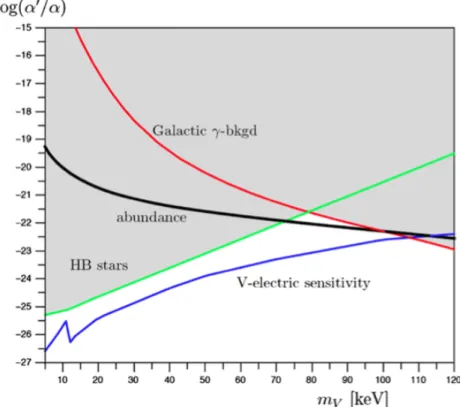
DM candidates with mass at the keV-scale must have a higher number density to compen-sate for their low mass and a correspondingly small, or super-weak interaction cross section to explain their as-yet non-detection. Their small mass and low energy render them difficult to detect via elastic nuclear scattering, as in the case of WIMPs, demotivating searches for fermionic keV-scale candidates such as the sterile neutrino or the gravitino. In contrast, the bosonic LDM detection principle is an inelastic interaction analogous to photoelectric absorp-tion. Assuming the particles are non-relativistic CDM candidates, a detection signal would be a peak with energy equal to the particle rest-mass. Recent LDM searches have focused on pseudoscalar and vector bosons since both existing and next-generation DM experiments could be competitive with astrophysical and cosmic gamma background constraints [76]. Figure 1.9 illustrates these constraints with possible sensitivity in Ge detectors.

For a bosonic pseudoscalar particle to be a viable keV-scale DM candidate, a couple assumptions related to coupling to the Standard Model must be made. The interaction term of the Lagrange density function looks like [76]:

Lint= Cγa

fa

FµνF˜µν−

∂µa

fa ¯

ψγµγ5ψ+... (1.11)

other fermions and gauge bosons. The term on the left in eqn. 1.11 is related to the two photon decay channel (e.g the Primakoff effect), while the term on the right is indicative of an axioelectric coupling. For viable keV-scale pseudoscalar DM without overly restrictive constraints onfA, we assume that the axioelectric coupling dominates while photon coupling is suppressed.

For keV-scale bosonic vector particles, the interaction Lagrange density can be written as [76]:

Lint =eκVµψγ¯ µψ+... (1.12)

which is an elementary vector interaction. Here e is the electronic charge, κ is the vector hypercharge, andVµis the vector field. The producte0 =eκ is analogous to electromagnetic coupling such that α0 = (eκ)2/4π is similar to a vector-electric fine-structure constant. Because it is assumed that the vector mass,mV is O(keV) instead of sub-eV, coupling with photons is suppressed3 [76, 77].

For experimentalists, a key difference between pseudoscalar and vector DM is their decays to photons. Since pseudoscalars are axion-like, their dominant decay mode is via the two photon decay. Vector decay into two photons is strictly forbidden. The dominant vector de-cay mode is to three photons. This has an impact on experimental sensitivity to bosonic DM candidates. Model dependent astrophysical constraints exclude the pseudoscalar parameter space that current experiments can probe, see for example [78, 79] and figure 6.3. For vec-tors, however, current experimental sensitivity is competitive with astrophysical constraints, see figure 1.9.

Bosonic scalar dark matter is not considered in this dissertation. The scalar-electric coupling term, which replaces the second term in eqn. 1.11, depends explicitly on the scalar mass. Scalar keV-scale DM thus requires highly model dependent parameters in order to be viable. Their phenomenology is also quite similar to the pseudoscalar boson.

3_{A more general form of the interaction term of the vector Lagrange density isL=κV}

Section 1.3: Outline of Dissertation

This dissertation will focus on the sensitivity of the MajoranaDemonstrator (MJD) to bosonic dark matter candidates. Since MJD is a P-type point contact (PPC) germanium detector array experiment, chapter 2 will provide an overview of semiconductor properties and PPC Ge detectors. Chapter 3 will discuss the overall Majorana Demonstrator experiment detailing construction, design, and cleanliness requirements. These first three chapters are meant to serve as an introduction, so that the reader becomes familiar with the experimental purpose.

CHAPTER 2: Semiconductor Detectors and the P-type Point-Contact Germanium Detector

This chapter provides an overview of Germanium detectors, with extra focus on p-type point-contact (PPC) detectors. To begin, a review of detection principles in semiconductor detectors1 is provided. The discussion will then shift to Germanium detectors, including some background on conventional detector configurations in order to lead into a discussion of PPC detectors. The remainder of the chapter will focus on PPC detectors, specifically their noise, resolution, and charge collection characteristics. The data presented in this dissertation was all acquired from the Majorana Demonstrator, which employs arrays of Ge PPC detectors.

Section 2.1: Properties of Semiconductor Detectors

2.1.1: Introduction

Ionizing radiation was discovered at the end of the 19th century. Early discoveries were made using photographic plates, commonly used in research during that time. In 1896, Henri Becquerel–after whom the S.I. unit of radiation is named–discovered that it’s possible to image certain phosphorescent materials on photographic plates even when the plates are covered by thick black paper. He concluded that invisible rays were emanating from these materials [80].

Detecting ionizing radiation with a semiconductor detector involves collecting ionized particles and/or liberated charge in a detector medium, usually by applying an electric field.

1_{These may also be referred to as solid-state detectors. While other types of detectors are technically}

Any liberated charge is collected by electrodes, hence a change in voltage or current across the electrodes indicates an ionizing event has taken place. Ideally, the response of the detector is a linear function of the incident energy deposit of the ionizing radiation.

Semiconductor detectors are widely used due to several advantages over other detectors types, such as gas-filled and scintillator detectors. Because semiconductors are made from denser and solid materials, they can more efficiently detect particles of higher energy, re-ducing the physical size of the detector. This includes gamma rays, for which many Ge detectors are optimized to detect. Another major advantage of semiconductor detectors is their superior energy resolution. Typically the energy resolution is limited by the statistical fluctuations in the number of charge carriers produced by incident radiation. In silicon and germanium, the energy required to create an electron-hole pair at 77 Kelvin (liquid nitrogen temperature) is 3.76 and 2.96 eV respectively [81, 82]. A typical Ge detector might have a resolution between 1-2 keV FWHM at 1173 keV (0.09-0.18%) [83], while the FWHM of a NaI scintillator detector might be roughly 60-70 keV (5-6%) [84].

2.1.2: The Band Gap Model

Figure 2.1: The band structure for insulators, semiconductors and conductors are shown. In insulators and semiconductors, the two bands are separated by the band gap energy,Eg. The

size ofEg determines whether a material is an insulator or semiconductor. In the absence of

thermal excitation, electrons in the valence band cannot jump to the conduction band and the material will have no conductivity. Also, in conductors, the conduction and valence bands overlap, allowing for the conduction of electrons.

33

Figure 2.1: A simplified band gap model of solids. The larger energy difference between the two insulator bands (left) prevent most electrons from crossing the gap. In semiconductors (middle), thermal excitation is much more likely to excite an electron into the conduction band. For metals (right), the conduction band overlaps the valence band resulting in some excess of mobile charge. Figure from [53].

If an electron gains sufficient energy to cross the gap a net positive charged vacancy, or hole, will be left in the valence band. This effect is generally referred to as electron-hole pair creation2. Both the electron and the hole will drift under the influence of an electric field in opposite directions and at different drift velocities that depend on the carrier mobility, equation 2.1 [82].

vh =µhE and ve =µeE (2.1)

where E is the electric field strength, v is the drift velocity, and µ is the field-dependent carrier mobility. Equation 2.1 breaks down at higher electric field strength; eventually the drift velocity reaches a saturation value, becoming independent of E.

The probability per unit time is that an electron-hole pair will be thermally generated is

given in equation 2.2 from [82]:

P(T) =CT32exp

− Eg 2kBT

(2.2)

where T is the temperature in Kelvin, Eg is the gap width, kB is the Boltzmann constant (k_B = 8.617×10−5 _{eV/K), andCis a proportionality constant inherent to the material. If no}

electric field is applied, the thermally produced electron-hole pairs will eventually recombine. An equilibrium pair concentration will be established that is proportional to the production rate. In germanium detectors, this concentration is too high at room temperature (293 K) due to the small gap width (0.665 eV), resulting in higher than acceptable leakage currents. For this reason, germanium detectors are commonly operated at LN temperature to reduce the thermal pair creation [85].

2.1.3: Impurities and Dopants

In a completely pure semiconductor there are an equal number of electrons and holes at any given time. Each electron promoted to the conductance band produces a hole in the valence band. The equilibrium concentration of holes and electrons, which depends on temperature and the gap energy width, will be the same. In reality, a 100% pure, or intrinsic, semiconductor is impossible to achieve. There will always be some residual impurities in the semiconductor that affects the intrinsic conductivity of the material.

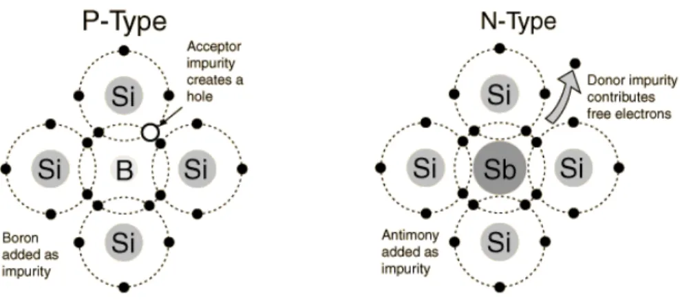
just below the conduction band. Similarly, a trivalent impurity, such as gallium or boron will introduce an additional acceptor site, or hole into the lattice. This manifests as an electron energy level slightly above the valence band. Figure 2.2 shows a simplified model of the effect of impurities in a semiconducting crystal.

Figure 2.2: Simplified model of impurities in a silicon crystal. In the p-type material (left), an acceptor site or hole is created because of the trivalent boron impurity. The antimony impurity in the n-type material (left) contributes a donor electron that is very weakly bound to the lattice site. Figure reprinted with permission from [86].

Doped semiconductors with more donor impurities are referred to as n-type semiconduc-tors while those with more acceptor impurities are designated as p-type. Electrons (Holes) are the majority charge carriers in n-type (p-type) materials. An impure semiconductor can be made to behave more like the intrinsic material by adding a compensating impurity of the opposite type. Heavily doped materials are often referred to with a ‘+’ superscript, e.g. a semiconductor heavily doped with acceptor impurity is p+-type. The importance of considering material type is examined in section 2.1.4.

2.1.4: Semiconductor Junction

immobile space charge (ionized lattice atoms) creates an electric field that opposes the further diffusion of free charge. This region of electric field is called the depletion region. Any negative (positive) charge that forms in the depletion region, e.g from ionizing radiation, is forced towards the n-type (p-type) material. In Ge, the potential difference across this region is roughly 0.4 V [83]. See figure 2.3.

Figure 2.3: Charge distribution at the junction of opposite type semiconductors. Majority carriers from the two types each diffuse into the opposite typed material. At equilibrium, the resulting electric field opposes further diffusion, creating a depleted region (center). Figure originally uploaded by user “TheNoise” to English Wikipedia under the CreativeCommons License.

doped than the p-type material, the depletion width can be estimated as [82],

d'p2µρV , V =V0+Vb.

(2.3)

where d is the depletion width, is the dielectric constant (= 120 in Ge), µ is the carrier

mobility, ρ is the resistivity of the material, and V is the voltage across the junction. Here

V is the sum of the intrinsic junction voltage V0 and the applied bias voltageVb. In practice, the bias voltage will be much larger than the junction voltage (∼1000 V compared to<1 V). The resistivity of the material is given by [82],

ρ= 1

eµN (2.4)

where e is the carrier charge and N is the charge carrier density. This implies that the depletion width increases with the purity of the material. In most applications, a depletion region that spans the length of the detector (∼few cm) while maintaining a reasonable bias voltage (< 5000 V) is desirable. The germanium used in the production of high purity Ge detectors have measured impurity levels as low as 1010 atoms/cm3 to achieve this [83].

Section 2.2: High Purity Germanium Detectors

2.2.1: Crystal Fabrication

Detectors are fabricated from electronic-grade polycrystalline germanium–a raw material of very high purity used by the electronics industry [83]. To further purify the germanium to high-purity grade, the process of zone refining is used. An ingot of germanium is placed in a crucible and heated using radio-frequency (RF) heating coils. The portions of the ingot closest to the coils then melts, increasing the mobility of the impurities. The heating coils are slowly moved down the length of the crucible, resulting in a moving melted zone of the ingot. The impurity concentration remains highest in the melted zone. Eventually the impurities are swept to the end of the ingot, which can then be cut off. Multiple passes through the zone refining coils are usually required to reach the desired concentration. Figure 2.4 show a vertical zone refining setup.

Figure 2.4: Vertical zone refining setup. The heating coil moves down the tube effectively dragging the impurities to the bottom of the crystal. Figure originally from [88], now in public domain.

seed crystal is a small piece of single crystal germanium from which the large crystal boule will grow. The size of the boule will depend on the temperature and how fast the crucible is pulled from molten germanium. The Czochralski crystal growing also serves as the final purification step in HPGe production, as impurities are removed with the excess crystal melt. Various techniques such as rotating the boule may be employed based on the experience of the crystal puller. Many of the parameters such as temperature and pull rate have to be precisely controlled by an experienced operator. For these reasons, the fine procedural details are often a commercial secret [83]. An simplified visualization outlining the process is shown in figure 2.5

Figure 2.5: A simplified figure of the Czochralski process. The end result is a cylindrical single crystal boule. Image from wikimedia commons, entered in public domain.

electric field during detector operation [82, 83].

Finally, the n+ and p+ contacts on the detector must be formed. The n+ contact on a p-type detector is made by diffusing lithium onto the surfaces. This is typically done on all surfaces with the exception of the base surface. Diffusion of lithium creates a dead-layer, a region of virtually constant electric potential in which no charge can be collected and thus no radiation can be detected. Typically this region is roughly 700µm thick. The p+ contact is usually made via boron implantation, and can be much thinner,∼0.3µm thick. Detectors designed for low-energy radiation detection (e.g. O(10 keV), x-ray) will have a larger p+

contact surface area that acts as a window for less penetrating radiations [83, 90].

2.2.2: Conventional Ge Detector Configurations

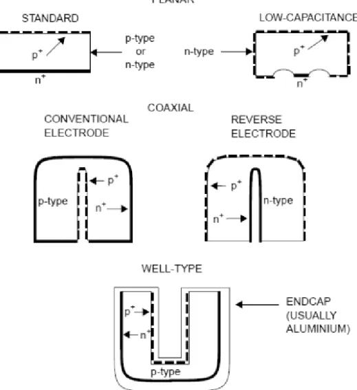
Two geometries are generally considered when configuring germanium detectors, the pla-nar geometry and the coaxial geometry. The detector configuration has a direct effect on important detector characteristics including resolution and charge collection. For reference, a brief description of the two types is given. A simple schematic of different detector config-urations is show in figure 2.6. A more in-depth overview of the P-type point contact (PPC) detector, a relatively recent configuration, can be found in section 2.3.

Planar Detectors

grounded, guard ring electrode can be included on the blocking contact face to minimize the current’s effect on the detector signal. Planar detectors range from 3 - 70 mm in diameter and up to 3 cm in height [82, 83].

Coaxial Detectors

Coaxial detectors are the most common type of germanium detectors in use. In this configuration, the electrical contact is made on the cylindrical surface of the detector. An axial bore is removed from the center of the detector to provide the opposite contact. Usually the inner bore does not go all the way through the crystal. Coaxial detectors have a better capacitance to volume ratio than planar detectors. A large volume is desirable in order to increase the gamma peak-to-Compton ratio and detection efficiency. Since germanium crystals are grown axially, it’s possible to produce very long coaxial detectors, with active volumes up to 800 cm3 [83, 85].

Section 2.3: PPC Detectors

The P-type point contact detector is the detector configuration of choice for the Majo-ranaDemonstrator, and has been deployed in multiple rare decays searches [53, 92, 93]. The geometry is similar to the low-capacitance planar detector in figure 2.6, however the detector is p-type, the rectifying electrode is n+ diffused lithium surrounding much of the detector, and the p+ blocking electrode is small, ∼3 mm in diameter point contact. The PPC detector configuration results in low-noise and superior resolution, along with charge collection properties that are well-suited for the pulse shape discrimination required by MJD.

2.3.1: Noise Characteristics

noise are considered, series and parallel white noise along with series and parallel non-white noise.

The series white noise, denoted by the spectral power density (i.e. the distribution of power over the frequency domain) term a [94], is caused by random thermal noise. It’s related to temperature and FET transconductance, gm by,

a=α2kT

g_m (2.5)

where k is the Boltzmann constant andα is a constant value between 0.5 and 0.7 depending on the FET operating point. There is also a non-white series 1/f term, af, which is related to charge trapping in the FET channel [92].

The spectral density of the parallel white noise is denoted, b. It is a shot (i.e poisson) noise related to the leakage current and to the thermal noise of the feedback resistor:

b =eIL+ 2kT

Rf

. (2.6)

Here e is the electron charge, IL is the leakage current and Rf is the feedback resistance. The term including the feedback resistance could be eliminated by using a pulsed-reset preamplifier, however detectors used in MJD have resistive feedback preamps. The amount of leakage current is generally indicative of the quality of detector and FET. Detectors with fewer impurities will exhibit less leakage current, see equation 2.4. The non-white parallel noise term bf/|f|, describes the dielectric noise [94].

After applying a filtered response in the Laplace domain, one can obtain the equivalent noise charge by summing the noise components [94, 95],

ENC2 =

aA1

τ + 2πafA2

C_tot2 +

bτ A3+ bf 2πA2

(2.7)

the filter shape, and C_tot is the combined detector and FET capacitance. Note that the non-white noise is independent of shaping time. During MJD data acquisition and analysis, a digital trapezoidal filter is applied [96]. The trapezoidal shaping coefficients are A1 = 2, A2 = 1.38, and A3 = 1.67 [95]. In this case, the shaping time includes the both trapezoidal

ramp times and the flat time. An example of the ENC2plotted versusτ is shown in figure 2.7.

15

Prototype String Readout Tests

22 May, 2012 Poon, MJD CD 2/3

•

HV, preamp controller and pulser board controlled by ORCA

•

Similar noise performance as the single detector unit

parallel series

non-white

Trapezoidal ramp time τ(µs)

FWHM

2 (e

V

2)

Figure 2.7: An example of the noise curve as a function of shaping time from a Majorana research PPC detector. The series, parallel and non-white noise contributions are shown (red-dashed). This is usually measured by finding the FWHM of a pulser peak to exclude the effect of charge production and collection. If white noise dominates, then the shaping time can be adjusted to minimize Equivalent Noise Charge. Figure generated by R. Martin, from [97].

In general, minimizing ENC2 is desired. Typically this involves adjusting the filter shap-ing time and measurshap-ing the electronic noise. The minimum achievable noise as a function of

τ can be found by simply taking the derivative and substituting. The resulting theoretical minimum is:

ENC2_min= 2 (abA1A3)

1 2 _C

tot+A2

2πafCtot2 + bf 2π

(2.8)

Equation 2.8 clearly shows the dependence of the noise on the total capacitance.

capacitance and the amplifying field-effect transistor (FET) capacitance [92, 98]:

FWHM = (41eV)Vn(CD +CF)/ √

τ (2.9)

where Vn is the FET noise voltage and τ is the characteristic time of the shaping amplifier. The capacitance of a PPC detector is given by [92, 99]:

CD = 2πGe0r (2.10)

where 0 = 8.85×10−12 Farad/m is the permittivity of free space, Ge is the germanium dielectric constant, and r is the point contact radius. Typical values for the PPC detector capacitance are ∼1 pF compared to ∼20 pF for a coaxial detector [99].

The low noise due to the small PPC capacitance also results in reduced energy thresholds. There is no standard method for setting detector thresholds. Experiments may simply set their threshold at five standard deviations above the noise pedestal or they might systemati-cally increment the threshold until background rates are reasonable. Equation 2.11 provides a stochastic rate based procedure for threshold finding [92, 100]:

R∼N₀eζ2/(2σ2) (2.11a)

N0 ∼

1

4τ (2.11b)

2.3.2: Detector Resolution

Energy resolution is one of the most important qualities of a detector. Germanium detectors are known for their superior energy resolution when compared to other detector types, (e.g ionization chambers or scintillators). For example, at 1.3 MeV the peak resolution for a coax detector is∼2 keV FWHM, while for a NaI scintillator the FWHM would be 25-30 times larger [83, 84]. PPC detectors perform better than coaxial detectors at low energies (x-ray regime) because they’re subject to less electronic noise. Other factors affecting the resolution must be considered as well, including statistical fluctuations in electron-hole pair production and charge collection efficiency.

The detected energy from a gamma radiation3 event is stochastically spread out over a narrow range. There are four processes that affect the energy resolution of HPGe detectors. When summed in quadrature, these yield the ultimate detector resolution:

σ_tot2 =σ2_γ+σ_p2+σ2_c+σ_e2 (2.12)

Each component is briefly described in the following list,

• σγ: Intrinsic gamma-ray width. This value is much smaller than the other uncertainties and is considered negligible.

• σp: Poisson fluctuations in the number of electron-hole pairs produced by an incoming gamma ray.

• σc: Spread of charges collected at the electrodes once the gamma ray energy has been fully absorbed by the detector

• σe: Electronic noise component. This was discussed in detail in section 2.3.1.

At low energies (< 500 keV), the electronic (σe) and production (σp) terms dominate

the contribution to the energy spread. The fluctuation in the number of electron-hole pairs produced as a function of energy is given by,

σn(E) =

p

hni=

s E

hεi. (2.13)

Multiplying by the average energy required to produce a pair (hεi= 2.96 eV) results in the uncertainty of the energy absorbed by the detector,

σp(E) = hεi ×

p

hni=phεiE. (2.14)

Note that equation 2.14 predicts a FWHM = 2.355×σ_p for the 60Co 1333 keV line of ∼4.7 keV, which is large compared to <2 keV FWHM quoted by detector manufacturers. The discrepancy arises from the original assumption modeling electron-hole pair creation as a poisson process. Each pair creation event is not necessarily independent of other events. The effect is accounted for by introducing the Fano Factor [102, 103], F:

σ_p(E) =phεiF E (2.15)

Typical measurements for F in Ge range from 0.057 to 0.12. Usually the measured Fano factor will be provided by the manufacturer on the detector data sheet.

At higher energies (>1000 keV), the charge collection spread has a noticeable impact on the resolution. Charges may become subject to trapping during collection. This results in tailing on the low energy side of the peak. The mathematical form of σ_c is not well understood and is often determined by measuring the total resolution and subtracting out the electronic and production components. In practice this term is modeled assuming a linear relationship with energy, such that σc = cE. A more in-depth discussion on charge collection and pulse shape discrimination is presented in section 2.3.3.

a function of energy,

σ_E(E) = pσ2

e+hεiF E+c2E2 (2.16)

where σe, F, and c are usually determined via a fitting routine. The FWHM of a set of known calibration peaks can be measured by a spectrometrist in order to fit equation 2.16. Knowing the resolution as a function of energy is necessary for setting limits in rare-event or low contamination settings. An example of a fit function is shown in figure 4.8.

2.3.3: Charge Collection in PPC Detectors

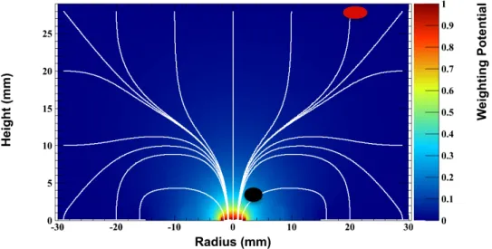
Ionizing radiation absorbed by a germanium detector liberates a collection of electron-hole pairs with total charge proportional to the incident energy. Under bias, an electric field permeates the detector so that holes migrate to the cathode–the point contact in a PPC detector–and electrons migrate to the anode. The field profile in a PPC detector affects the collection timing characteristics. If a gamma ray were to deposit energy at two different sites in the crystal, an appreciable delay in the induced charge signal may be discernible. Pulse shape discrimination techniques can identify charge collection delay, discriminating between these ‘multi-site events’ and single-site events. If energy is deposited near the detector dead layer, i.e close to the surface in regions of low electric field, the charge collection time could increase significantly, resulting in energy-degraded slow pulses. In contrast, charge drift times in coaxial detectors are fairly uniform throughout the crystal volume. See figure 2.8.

The output signal from a PPC detector can best be understood by applying the Shockley-Ramo theorem [105, 106]. The theorem provides a method for calculating the charged induced on the electrodes as electron-hole pairs drift through the detector. Each electrode is considered independently. The induced current on an electrode related to the drift velocity,

vd, and the weighting field strength,E0,