AUTOMATIC LOCALIZED ANALYSIS OF LONGITUDINAL CARTILAGE CHANGES
Liang Shan
A dissertation submitted to the faculty of the University of North Carolina at Chapel Hill in partial fulfillment of the requirements for the degree of Doctor of Philosophy in
the Department of Computer Science.
Chapel Hill 2014
c 2014 Liang Shan
ABSTRACT
Liang Shan: AUTOMATIC LOCALIZED ANALYSIS OF LONGITUDINAL CARTILAGE CHANGES
(Under the direction of Marc Niethammer)
Osteoarthritis (OA) is the most common form of arthritis; it is characterized by the loss of cartilage. Automatic quantitative methods are needed to screen large image databases to assess changes in cartilage morphology. This dissertation presents an auto-matic analysis method to quantitatively analyze longitudinal cartilage changes from knee magnetic resonance (MR) images.
A novel robust automatic cartilage segmentation method is proposed to overcome the limitations of existing cartilage segmentation methods. The dissertation presents a new and general convex three-label segmentation approach to ensure the separation of touch-ing objects, i.e., femoral and tibial cartilage. Anisotropic spatial regularization is intro-duced to avoid over-regularization by isotropic regularization on thin objects. Temporal regularization is further incorporated to encourage temporally-consistent segmentations across time points for longitudinal data.
TABLE OF CONTENTS
LIST OF FIGURES . . . vii
LIST OF TABLES . . . ix
CHAPTER 1: INTRODUCTION . . . .1
1.1 Motivation . . . .1
1.2 Cartilage segmentation . . . .3
1.2.1 Existing methods. . . .4
1.2.2 Proposed method. . . .9
1.3 Cartilage thickness analysis . . . 11
1.3.1 Existing methods. . . 12
1.3.2 Proposed method. . . 12
1.4 Thesis and contribution . . . 13
1.5 Overview of chapters . . . 14
CHAPTER 2: THREE-LABEL SEGMENTATION . . . 16
2.1 Introduction . . . 16
2.2 Related work . . . 17
2.3 Three-label segmentation. . . 19
2.3.1 Limitation of binary segmentations . . . 20
2.3.2 A general three-label segmentation method . . . 21
2.3.3 Three-label segmentation with isotropic regularization . . . 23
2.3.4 Three-label segmentation with anisotropic regularization . . . 24
2.4 Multi-label segmentation . . . 27
2.4.1 Limitation of three-label segmentation . . . 27
2.4.2 Multi-label segmentation . . . 27
2.4.3 Numerical solution . . . 34
2.5 Conclusion . . . 35
CHAPTER 3: AUTOMATIC MULTI-ATLAS-BASED THREE-LABEL CARTILAGE SEGMENTATION . . . 37
3.1 Introduction . . . 37
3.2 Atlas-based segmentation . . . 41
3.3 Multi-atlas-based bone segmentation . . . 42
3.4 Probabilistic classification . . . 43
3.4.1 Classification using kNN . . . 44
3.4.2 Classification using an SVM. . . 45
3.5 Average-shape-atlas-based cartilage segmentation . . . 45
3.6 Multi-atlas-based cartilage segmentation . . . 46
3.7 Overall segmentation pipeline . . . 49
3.8 Conclusion . . . 50
CHAPTER 4: VALIDATION OF CARTILAGE SEGMENTATION . . . 52
4.1 Introduction . . . 52
4.2 Data description. . . 52
4.3 Bone validation. . . 53
4.4 Cartilage validation . . . 55
4.5 Comparison to other methods . . . 64
4.5.1 Comparisons based on the SKI10 dataset . . . 64
4.5.2 Qualitative comparison to other methods . . . 71
CHAPTER 5: LONGITUDINAL THREE-LABEL CARTILAGE
SEGMENTATION . . . 72
5.1 Introduction . . . 72
5.2 Longitudinal three-label segmentation. . . 73
5.2.1 Numerical solution . . . 73
5.3 Registration of longitudinal images. . . 75
5.4 Experimental results . . . 77
5.5 Conclusion . . . 79
CHAPTER 6: LOCALIZED ANALYSIS OF LONGITUDINAL CARTILAGE THICKNESS . . . 82
6.1 Introduction . . . 82
6.2 Cross-sectional vs. longitudinal analysis. . . 83
6.2.1 Cross-sectional analysis of longitudinal data . . . 84
6.2.2 Linear mixed effects model for longitudinal data . . . 86
6.3 Spatial correspondence of cartilage thickness . . . 88
6.4 Longitudinal analysis of localized cartilage thickness changes . . . 88
6.5 Experimental results . . . 93
6.5.1 Results of femoral cartilage . . . 94
6.5.2 Results of tibial cartilage . . . 95
6.5.3 Comparison to regional analysis. . . 102
6.6 Conclusion . . . 110
CHAPTER 7: DISCUSSION . . . 112
7.1 Summary of contributions . . . 112
7.2 Future work . . . 115
LIST OF FIGURES
1.1 MR image of the knee.. . . .2
1.2 Cartilage segmentation pipeline. . . 10
2.1 Compare binary and three-label segmentations. . . 20
2.2 Functionu and |∇lu| for three-label segmentation. . . 23
2.3 Compare isotropic and anisotropic regularization. . . 24
2.4 Difference between isotropic and anisotropic regularization. . . 25
2.5 Regularization bias of isotropic three-label segmentation. . . 28
2.6 No regularization bias of isotropic multi-label segmentation. . . 29
2.7 Regularization bias of anisotropic three-label segmentation. . . 30
2.8 No regularization bias of anisotropic multi-label segmentation. . . 31
2.9 Functionu and ∇lu for each object. . . 33
3.1 Cartilage segmentation pipeline. . . 40
4.1 Box plots of DSC for bone segmentation. . . 54
4.2 Bone segmentation of one example slice in coronal view. . . 54
4.3 Compare binary and three-label segmentation methods.. . . 55
4.4 Average atlas built from 18 images. . . 56
4.5 Cartilage segmentation of one example slice in coronal view. . . 57
4.6 Compare kNN and SVM for the femoral cartilage. . . 57
4.7 Compare kNN and SVM for the tibial cartilage.. . . 58
4.8 Compare different atlas choices with isotropic regularization. . . 59
4.9 Compare different atlas choices with anisotropic regularization. . . 60
4.10 Improvement by anisotropic regularization.. . . 61
4.12 Boxplots of DSC for different KLG. . . 62
4.13 Scatter plots of segmentation volumes . . . 63
4.14 Correlation coefficients of local cartilage thickness. . . 63
4.15 Box plots of segmentation measures from SKI10 methods. . . 66
4.16 An example slice from SKI10 training dataset. . . 70
5.1 Benefit of longitudinal segmentation. . . 74
5.2 Mean DSC over temporal regularization. . . 78
5.3 Box plots of TCM from different segmentations. . . 80
6.1 Thickness computation pipeline. . . 89
6.2 Examples of 2D cartilage thickness maps. . . 90
6.3 Analysis (before clustering) of FC with expert segmentations. . . 96
6.4 Analysis (before clustering) of FC with independent segmentations.. . . 97
6.5 Analysis (before clustering) of FC with longitudinal segmentations. . . 98
6.6 Analysis (after clustering) of FC with expert segmentations. . . 99
6.7 Analysis (after clustering) of FC with independent segmentations. . . 100
6.8 Analysis (after clustering) of FC with longitudinal segmentations. . . 101
6.9 Analysis (after clustering) of FC with longitudinal segmentations. . . 102
6.10 Analysis (before clustering) of TC with expert segmentations. . . 103
6.11 Analysis (before clustering) of TC with independent segmentations. . . 104
6.12 Analysis (before clustering) of TC with longitudinal segmentations. . . 105
6.13 Analysis (after clustering) of TC with expert segmentations. . . 106
6.14 Analysis (after clustering) of TC with independent segmentations. . . 107
6.15 Analysis (after clustering) of TC with longitudinal segmentations. . . 108
6.16 Analysis (after clustering) of TC with expert segmentations. . . 109
LIST OF TABLES
4.1 Validation of bone segmentation. . . 53
4.2 Validation of cartilage segmentation. . . 63
4.3 Results of statistical tests between SKI10 methods. . . 67
4.4 DSC from the SKI10 methods. . . 68
CHAPTER 1: INTRODUCTION
1.1 Motivation
Osteoarthritis (OA) is the most common form of arthritis and is a major cause of long-term disability in the US (Woolf and Pfleger, 2003). It is estimated that more than 16% of all adults 45 years or older suffer from symptomatic OA of the knee (CDC, 2008). The OA symptoms include swelling, pain, discomfort and problems in mobility and are caused by the progressive loss of joint cartilage (CDC, 2008). Figure 1.1 shows the anatomy of the human knee and illustrates the cartilage loss. While current treatment options help control pain, they are not able to reverse disease progression (Felson et al., 2000b). Further drug research is essential to help OA patients.
(a) (b) (c)
Figure 1.1: Example slice from T1 weighted MR images of human knee and illustration of cartilage loss. (a) A sagittal slice from a 3-dimensional T1 weighted MR image of a healthy knee. Bones are annotated in blue, femoral cartilage in purple and tibial cartilage in orange. (b) A coronal slice from the same MR image. (c) A coronal slice of an OA knee with cartilage loss indicated by the red arrow.
Eckstein et al., 2006). Therefore, MRI is increasingly accepted as a primary method to evaluate progression of OA (Raynauld, 2003; Raynauld et al., 2004; Cicuttini et al., 2005).
Large image databases have been acquired for OA research. For instance, the database of the Osteoarthritis Initiative (Peterfy et al., 2008) contains MR image data for 4,796 subjects. The Pfizer Longitudinal Study (PLS) (Eckstein et al., 2008), a case-control study, consists of 97 normal control and 61 OA subjects. It would be of great value to fully analyze the MR images of these datasets in understanding the progression of OA. This would require robust fully-automatic computer-assisted image analysis methods because even if only a small amount of human intervention is needed for a single image, it would be extremely labor-intensive to analyze (tens of) thousands of images. Therefore a fully-automatic cartilage segmentation and longitudinal analysis from MR images is crucial to study OA.
correspondence and statistical analysis of longitudinal changes, among which the seg-mentation and the statistical analysis are the most challenging components. Cartilage registration is not a trivial task either because of the small size of the cartilage.
1.2 Cartilage segmentation
Automatic cartilage segmentation is a challenging problem in the field of medical image analysis for the following reasons.
1. Cartilage is a small and thin structure. There are many other tissues, e.g., muscles, in the MR image, which are irrelevant for the assessment of cartilage. This makes
a fully-automatic segmentation challenging.
2. A segmentation method needs to be robust enough to be applied to large image datasets exhibiting variations in image appearance.
3. Femoral and tibial cartilage appear to be touching in an MR image, so conventional binary segmentation would merge them into a single object. Therefore, a new segmentation method is needed to produce separate segmentations for touching
objects.
4. Isotropic spatial regularization as a means to deal with noisy image data is not an ideal choice for cartilage segmentation because it tends to shrink the segmentation boundary by cutting thin objects short.
1.2.1 Existing methods
Automatic cartilage segmentation in the knee has been researched for decades. Many segmentation approaches have been proposed with varying levels of automation, e.g., region growing methods (Adams and Bischof, 1994), watershed methods (Beucher and Meyer, 1993), live wire (Mortensen and Barrett, 1995), active contours (Kasset al., 1988; Caselles et al., 1997a), model-based segmentation methods (Cootes et al., 1995, 2001), graph-based methods (Felzenszwalb and Huttenlocher, 2004; Boykov and Kolmogorov, 2004), pattern recognition methods (Dudaet al., 2001), and atlas-based methods (Aljabar
et al., 2009). However, all the methods suffer from certain shortcomings, which are
discussed below. A novel automatic segmentation method is proposed in this thesis to address the issues of the existing methods.
Region growing methods
The region growing algorithm (Adams and Bischof, 1994) iteratively examines neigh-boring pixels of “seed points” and determines whether the pixel neighbors should be added to the region. The method requires manual interaction to obtain the seed points and suffers from its sensitivity to image noise and parameter settings. Peterfy et al.
(1994), Piplani et al. (1996), Eckstein et al. (1996, 1998) and Tamez-Pena et al. (1999) applied region growing methods to obtain semi-automatic cartilage segmentations.
Watershed methods
basins of the drops of water. Generally, the watershed transform is computed on the gra-dient magnitude image, so the boundaries are located at high gragra-dient pixels. The main drawbacks of the watershed transform (Grau et al., 2004) are over segmentation, sensi-tivity to noise, poor detection of areas with low contrast boundaries and thin structures. Ghosh et al. (2000) and Grau et al. (2004) used watershed method for semi-automatic
cartilage segmentation.
Live wire
The live wire (also known as intelligent scissors) (Mortensen and Barrett, 1995) is an interactive segmentation method which allows the user to choose a contour by roughly tracing the object boundary. The local minimum cost path from the current cursor position to the last seed point is computed. Additional user interaction is needed if the computed path deviates from the desired one. The major limitation of this method is that heavy user interaction is necessary when many alternative minimal paths may exist. This method was applied by Steineset al.(2000) and Gougoutaset al.(2004) to compute
semi-automatic cartilage segmentation in a slice-by-slice manner.
Active contours
An active contour model, also known as a snake, is an energy-minimizing spline guided by external constraint forces and influenced by image forces that pull it toward features such as lines and edges (Kass et al., 1988). The active contour method had a tremen-dous impact in the segmentation community. The original formulation is not geometric, meaning there is not obvious relation between the parametrization of the contour and the geometry of the objects to be captured (Angenent et al., 2006). Many extensions to and variations of the snakes have been proposed to address this issue. Caselles et al.
weighted length of a closed curve. The curve that minimizes the weighted length will prefer to be on the image edges. Despite the popularity of these methods, most active contour methods suffer from a major drawback, high sensitivity to initialization, which is related to the non-convexity of the energy functional. The segmentation algorithm tends to get stuck in undesired local minima. Lynchet al. (2000), Kauffmannet al. (2003) and
Brem et al.(2009) reported semi-automatic cartilage segmentation methods with active
contour models.
The initial implementations of active contours used parameterizations which lead to non-convex optimization problems. More modern approaches (Appleton and Talbot, 2006) are more closely related to graph-cuts and are based on convex energy functions (see below).
Graph-based methods
Graph-based image segmentation techniques (Felzenszwalb and Huttenlocher, 2004) represent an image using a graph where each node corresponds to a pixel in the image and the edges connect certain pairs of neighboring pixels. A weight is associated with each edge based on some property of the pixels that it connects, such as image intensities. Then a segmentation corresponds to a cut of the graph. A global optimal solution may be obtained for graph cuts. Boykov and Kolmogorov (2004) presented an efficient way to compute the max-flow for computer vision related graph. The graph-based methods, partitioning the image with a graph cut, solve essentially the same optimization problem as active contours, which uses a curve to separate objects. However, the solution method is fundamentally different because one searches a labeling of graph nodes rather than the location of a contour as in the traditional ways of implementing active contours.
Shimet al.(2009) and Baeet al.(2009) utilized graph cuts to achievesemi-automatic
(2010b) proposed a method for simultaneous segmentation of multiple interacting objects, named LOGISMOS (layered optimal graph image segmentation of multiple objects and surfaces). The method incorporates multiple spatial inter-relationships in a single n -dimensional graph. Yin et al. (2010b) also presented an automatic method to segment cartilage using LOGISMOS.
Graph-based methods generally suffer from grid bias, also known as metrication er-rors. Large neighborhood systems are required to remove the bias, but they result in a large number of edges and thus increase the memory consumption.
Model-based methods
In model-based segmentation, a statistical model is trained from a population of manual segmentations. The segmentation of a target image is computed iteratively. The model is fit to the target image and then refined based on the model and image features. Active shape models (ASM) (Cooteset al., 1995) and active appearance models (ASM) (Cootes et al., 2001) are the most frequently employed methods. Solloway et al.
(1997) used ASM to segment femoral cartilage in a semi-automatic way. Vincent et al.
(2010) applied AAM to computeautomatic cartilage segmentation. Glockeret al.(2007) and Seim et al. (2010) proposed different statistical shape models for bone/cartilage segmentation.
Despite the wide application, these model-based methods are prone to local min-ima in the fitting process. In addition, these models are usually restricted to a given shape/appearance space and hence may not be able to capture pathologies well.
Pattern recognition methods
(2007) proposed an automatic hierarchical voxel classification scheme using kNN. Dam and Loog (2008) accelerated the process through sparse classification. A support vec-tor machine (SVM) (Cortes and Vapnik, 1995) constructs a hyperplane, which has the largest distance to the nearest training data point of any class, in a high-dimensional feature space for classification. Koo et al. (2009) proposed to use SVM to segment car-tilage automatically from multi-contrast MR images. The spatial interactions between neighboring pixels are neglected in these methods. Nevertheless, it is straightforward to use these classifiers in combination with other methods. For example, one can use them to get likelihoods for foreground and background, which can then be used as unary terms in graph-cuts, and so on.
Atlas-based methods
An atlas (Aljabar et al., 2009), in the context of atlas-based segmentation, is defined as the pairing of an original structural image and the corresponding segmentation. Atlas-based segmentation methods can be categorized into three groups (Iˇsgum et al., 2009), namely single-atlas-based, average-shape atlas-based and multi-atlas-based methods. A statistical atlas was constructed by Glocker et al. (2007) for the patella cartilage from a set of pre-registered training images. The segmentation is solved through a single registration and thus is not robust to occasional registration failures.
In multi-atlas-based segmentation, multiple labeled images are registered to the query image independently. The propagated atlas labels are then fused into a single segmenta-tion of the query image. This results in a method which is more robust to registrasegmenta-tion failures than single-atlas-based and average-shape-atlas-based segmentation methods, both of which need only one registration. The downside of multi-atlas-based segmen-tation is the high compusegmen-tation cost since it needs multiple registrations. Rohlfing et al.
other two types of atlas-based segmentation methods. In spite of the expensive com-putation, multi-atlas-based segmentation has been quite popular and successful in brain imaging (Aljabar et al., 2009). Tamez-Pe˜na et al. (2012) reported a multi-atlas-based cartilage segmentation approach.
1.2.2 Proposed method
I propose a novel automatic cartilage segmentation method which has the following advantages. First of all, the method is fully automatic and requires no user in-teraction (besides quality control). Secondly, the method isrobust as it benefits from the multi-atlas-based strategies. Thirdly, both spatial and local appearance information are utilized in the segmentation. Local tissue classification is probabilistic (unlike Folkesson
et al.(2007), Dam and Loog (2008) and Kooet al.(2009)), and it is combined with a
spa-tial prior to generate the final segmentation within a segmentation model. Furthermore, the segmentation model isconvex and thus allows for the computation of global optimal solutions, which cannot be guaranteed by active contour models (traditional implemen-tations), ASM or AAM. The continuous formulation of the segmentation model makes the method free of grid bias that graph-based methods suffer from. The segmentation model also allows for the incorporation of spatial and temporal regularization.
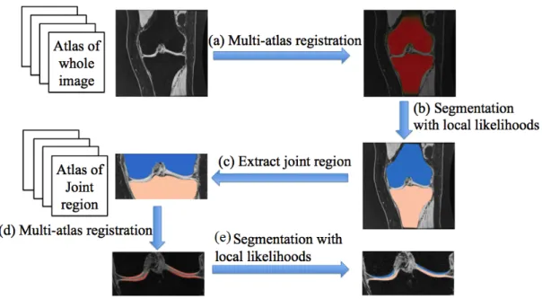
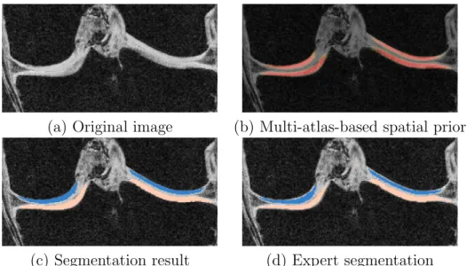
Figure 1.2: Cartilage segmentation pipeline. (a) Multi-atlas registration to compute the spatial prior for the bone. (b) Compute bone segmentation from the spatial prior and the local likelihood. (c) Extract the joint region. (d) Multi-atlas registration (based on bone segmentations) to compute the spatial prior for the cartilage. (e) Compute cartilage segmentation from the spatial prior and the local likelihood.
decision of the multi-atlas spatial priors and local likelihoods from a probabilistic tissue classification. Figure 1.2 shows the pipeline of multi-atlas cartilage segmentation.
The segmentation model for computing cartilage segmentation at step (e) in Fig. 1.2 is critical because the femoral and tibial cartilage appear to be touching in the MR image and it is desirable to separate them. Since binary segmentation methods tend to merge touching objects into a single one, I propose a general three-label segmentation approach which guarantees the separation of touching objects. The three-label seg-mentation is formulated as a convex optimization problem and therefore allows for the computation of global optimal solutions. The method is general, and it can be applied to other segmentation problems with two touching objects.
Therefore,I propose an anisotropic spatial regularization for cartilage segmen-tation and demonstrate it improves the segmentation accuracy in comparison to the isotropic one.
Temporally-consistent segmentation is desirable to study longitudinal change because subtle changes might be indicative of the disease. A longitudinal three-label seg-mentation is proposed to encourage temporal consistency across segmentations for longitudinal data. The longitudinal segmentation method is also general, and it can be applied to other segmentation problems with longitudinal data of two touching objects.
1.3 Cartilage thickness analysis
Statistical analysis of cartilage thickness changes is also achallenging problem for the following reasons.
1. Observational studies have shown that cartilage loss in OA may not be uniform throughout the cartilage but may affect certain regions (e.g., the center) more fre-quently and more strongly than others (Biswalet al., 2002). Therefore, a localized analysis method is necessary to understand localized cartilage thinning. The local-ized analysis requires establishing spatial correspondence across time and subjects which is challenging, due to the small spatial amount of cartilage.
1.3.1 Existing methods
Wirth and Eckstein (2008) studied average cartilage thickness change in defined anatomic subregions of the femorotibial joint. The tibial cartilage was divided into a central area of the total subchondral bone area and into anterior, posterior, internal, and external subregions surrounding it. In the weight-bearing femoral cartilage, central, internal, and external subregions were determined. However, this approach may be prob-lematic because changes within a specific subregion could happen only to a few subjects whereas other subjects have strong progressions in different subregions.
Buck et al. (2009) proposed to use ordered values of subregional change in each
subregion to focus on the thickness change alone regardless of in which subregion the change occurs in each subject. The ordered value approach was demonstrated to provide improved discrimination between healthy subjects and OA participants longitudinally. But the ordered value approach still relies on subdivisions of the cartilage and the average thickness within each subregion.
The subdivisions of the cartilage are purely geometric and necessarily coarse. Local changes (that happen to a smaller region than the size of a subregion) are weakened by averaging over a particular subregion and are impossible to recover. To fully understand the spatial pattern of OA progression, the analysis oflocalized cartilage thickness changes is necessary.
Williams et al. (2010) built spatial correspondence of cartilage thickness maps and studied local cartilage thickness. The method however treated all OA subjects equally without considering the spatial heterogeneity.
1.3.2 Proposed method
a method to establish spatial correspondence of cartilage thickness maps be-tween subjects and across time points. The cartilage thickness is computed from the obtained cartilage segmentation using a Laplace-equation approach (Yezzi and Prince, 2003) and then transformed to a common (the atlas) space based on the bone segmenta-tion. The cartilage thickness maps are then comparable across time points and between subjects.
Statistical analysis on localized cartilage changes is also challenging due to the fact that cartilage thinning may happen at different locations for different subjects. The heterogeneity of the longitudinal changes is not uncommon in the progression of other diseases. I propose a novel method to analyze the localized cartilage changes, which can also be applied to study nonuniform local morphological changes in other disease. I first identify the thinning locations for each subject and then group subjects into different clusters based on their thinning locations. The group difference between normal control and OA subjects will be studied at each thinning location.
1.4 Thesis and contribution
Thesis: Automatic, robust and accurate cartilage segmentations can be obtained through multi-atlas-based registration and local tissue classification within a three-label
segmenta-tion framework allowing for spatial and temporal regularizasegmenta-tion. Spatially transforming
cartilage thickness maps into an atlas space enables statistical analysis on localized
car-tilage changes. Clustering of OA subjects improves statistical analysis due to the spatial
heterogeneity of cartilage loss.
The scientific contributions are as follows:
allows for the computation of global optimal solutions. The method can be applied to other segmentation problems with two touching objects.
2. I validate the automatic three-label cartilage segmentation on a sizable dataset con-sisting of more than 700 images. Specially, I study the impacts of different types of atlases (namely average-shape-atlas and multi-atlas) and different types of reg-ularization (i.e., isotropic spatial regreg-ularization, anisotropic spatial regreg-ularization and temporal regularization) on cartilage segmentation accuracy.
3. I propose a novel method to analyze nonuniform localized cartilage changes, which can be applied to study nonuniform local morphological changes in other diseases.
4. I perform statistical analysis on a sizable longitudinal dataset containing about 150 subjects with 5 time points. The statistical analysis result of localized cartilage changes is presented and compared to that reported in literature using regional analysis.
The engineering contributions are the following:
1. I develop a new fully automatic three-label cartilage segmentation pipeline based on multi-atlas registration and local tissue classification.
2. I develop a method to establish spatial correspondences of knee cartilage across time points and between subjects, which allows for statistical analysis on localized cartilage thickness changes.
1.5 Overview of chapters
The remainder of this dissertation is organized as follows:
Chapter 3 applies the proposed three-label segmentation to obtain automatic cartilage segmentation through multi-atlas-based registration and local tissue classification.
Chapter 4 presents the validation of the proposed cartilage segmentation method and compares the proposed method to existing methods.
Chapter 5 discusses the computation of cartilage thickness, transforming the cartilage thickness maps into an atlas space, proposes a new clustering-based statistical method, and presents the results of applying the new method on localized cartilage thickness changes.
CHAPTER 2: THREE-LABEL SEGMENTATION
2.1 Introduction
Image segmentation is a fundamental problem in the field of computer vision and medical image analysis. It is an essential component towards, for example, automated vision systems and medical applications. The aim is to find a partition of an image into a finite number of semantically important regions. Two classes of methods have gained tremendous popularity in the past decades. One class is active contour methods, including snakes (Kass et al., 1988) and geodesic active contours and surfaces (Caselles et al., 1997a,b). The other class takes a different approach by transforming the segmentation problem to a graph problem, e.g., graph cuts (Ford and Fulkerson, 1962).
1998). In spite of the advent of these heuristics, active contours typically require manual intervention which limits their application.
Graph-based image segmentation techniques (Felzenszwalb and Huttenlocher, 2004) represent an image using a graph where each node corresponds to a pixel in the image and the edges connect certain pairs of neighboring pixels. A weight is associated with each edge based on some property of the pixels that it connects, such as image intensities. Then a segmentation corresponds to a cut of the graph. A global optimal solution may be obtained for graph cuts. Boykov and Kolmogorov (2004) presented an efficient way to compute the max-flow. However, graph cuts suffer from discretization artifacts, which typically result in a preference for contours and surfaces to travel along the grid directions. Large neighborhood systems are required to remove the bias but results in a large number of edges and thus increase the memory consumption. Also, parallel implementations are not straightforward (Delong and Boykov, 2008).
2.2 Related work
Chan-Vese segmentation (Chan and Vese, 2001) aims at finding an optimal image partition into a uniform foreground and background region. It is classically formulated as a curve/surface-based optimization problem of the form
E(c1, c2, C) =Length(C) +λ1
Z
inside(C)
(c1−I(x)) 2
dx+λ2
Z
outside(C)
(c2−I(x)) 2
dx (2.1) whereI(·) denotes image intensities,xis a pixel/voxel location,c1andc2 are the intensity
Appleton and Talbot (2006) recast active contours as a convex optimization problem by formulating the problem with respect to a labeling (indicator) function for foreground and background rather than with respect to a boundary curve/surface. Their approach can efficiently compute globally minimal curves and surfaces for image segmentation, stereo reconstruction, and other labeling problems. The method is isotropic (graph cuts are grid-biased) and optimal (active contours are suboptimal). The algorithm produces a globally maximal continuous flow at convergence. The energy functional Appleton and Talbot (2006) minimized is
E(u) = Z
Ω
g(x)dxwith seed points, u∈[0,1] (2.2)
where Ω is the spatial domain of the image, x is a pixel/voxel location in Ω. Here, u is a essentially binary labeling function for foreground (u = 1) and background (u = 0). And g is an edge-indicator function, small at edges and large in uniform regions. The globally optimal solution u can be computed efficiently. The globally minimal surface can be obtained trivially from the optimal u.
Bresson et al. (Bressonet al., 2007) proposed the following convex functional for seg-mentation based on the Chan-Vese energy (Chan and Vese, 2001) to optimally partition the image into piecewise constant regions:
E(u) = Z
Ω
gk∇uk dx+λ
Z
Ω
r
z }| {
(c1−I(x))2−(c2−I(x))2
u dx, u∈[0,1]. (2.3)
where I(·) denotes image intensities, c1 and c2 are the mean intensity estimates for the
is convex when the c1 and c2 are fixed. Chan-Vese method is not convex because c1 and c2 are optimized jointly with the segmentation.
In Shan et al.(2010), I proposed a novel binary segmentation extending the work by Bresson et al. The region-based term r in (2.3) can be reformulated in a probabilistic way. One can replace r by log Pi
Po with Pi and P0 probabilities of a pixel belonging to
foreground and background respectively (where equal Gaussian probability distributions result in the Chan-Vese energy).
To encourage segmentation stop at the desired boundary, a feature fieldFis added to favor boundaries with inward normal directions aligned with F itself. Thus, the overall optimization problem is to minimize the following convex energy functional
E(u) = Z
Ω
gk∇uk+ru+F· ∇u dΩ, r= log Po
Pi. (2.4)
The vector field F can be rewritten using the divergence theorem and integrated into the regional term r. The resulting segmentations are independent of initializations of function u due to the convexity of energy functional (2.4).
All the methods discussed above result in binary segmentations, in which each pixel is labeled either foreground or background. Multi-label segmentation assigns distinct labels to different foreground objects and therefore allows for distinction among objects of interest. In the next section, I will discuss the advantage of multi-label segmentation through a synthetic example and present a three-label segmentation framework.
2.3 Three-label segmentation
(a) (b)
Figure 2.1: Synthetic example comparing binary and three-label segmentations. (a) Bi-nary segmentation result. Femur and tibia are segmented as one object and the boundary in the joint region is not captured well due to regularization effects. (b) Proposed three-label segmentation. The boundaries between bones and background are preserved.
2.3.1 Limitation of binary segmentations
2.3.2 A general three-label segmentation method
The three-label case is a specialization of the multi-label segmentation method by
Zachet al.(2009). Using three labels allows for a symmetric formulation with respect to
the background segmentation class.
A multi-label segmentation is a mapping from an image domain Ω to a label space represented by a set of non-negative integers, i.e. L = {0, ..., L−1}. The labeling function Λ : Ω → L,x 7→Λ (x) maps a pixel x in the image domain Ω to label Λ (x) in label space. The goal is to find a labeling function that minimizes an energy functional of the form:
E(Λ) = Z
Ω
c(x,Λ(x)) +V(∇Λ,∇2Λ, ...) dx, (2.5)
where c(x,Λ(x)) is the cost of assigning label Λ(x) to pixel xand V(·) is a regularizing term. This optimization problem is generally difficult to solve as the data costs are typ-ically highly non-convex. By embedding the labeling assignment into higher dimensions and appropriately restating the energy (2.5), a convex formulation can be obtained.
The different labelings can be encoded through a level function u defined in higher dimensions
u(x, l) =
1 if Λ(x)< l, 0 otherwise,
(2.6)
which maps the Cartesian product of the image domain Ω and the labeling space L to {0,1}. By definition, we have u(x,0) = 0 and u(x, L) = 1. Of note, u does not directly encode labels, but instead defines them through its discontinuity set. Figure 2.2 illustrates the relation between uand Λ for the three-label case.
With the level function u, the label cost term can be rewritten as
Z
Ω
c(x,Λ(x)) = Z
D
using the same technique as Pock et al. (2008) proposed. The regularization energy in 2.5) can be written in terms of the gradient of the level function as
Z
D
ψx,l(∇u)dxdl, D= Ω× L, (2.8)
where ψx,l defines the regularization term and is convex and 1-positively homogeneous.
By combining the two terms, one can rewrite (2.5) purely in terms ofu,
E(u) = Z
D
ψx,l(∇u) +c(x, l)|∇lu(x, l)| dxdl, D = Ω× L. (2.9)
As u can only take two integer values, i.e., 0 and 1, the functional (2.9) is not convex. The non-convex constraint is usually relaxed to a convex one onu∈[0,1]. The relaxation transforms the original hard optimization problem into a related problem that is convex and therefore easier to solve. Zach et al. (2009) has proven that the resulting solution
u to the relaxed problem is essentially binary and thresholding of an essentially binary optimal solution of energy (2.9) yields to an equally globally optimal solution to the original discrete problem.
(a) ufor Λ = 0 (b) ufor Λ = 1 (c) u for Λ = 2
(d) |∇lu| for Λ = 0 (e) |∇lu| for Λ = 1 (f) |∇lu| for Λ = 2 Figure 2.2: Values ofu and |∇lu|for different label assignments in a three-label segmen-tation (abscissal). Assuming a discretization with forward differences. |∇lu|determines the label assignment.
2.3.3 Three-label segmentation with isotropic regularization
The three-label segmentation energy functional is formulated as (the explicit depen-dence of xand l is omitted)
E(u) = Z
D
gk∇xuk+c|∇lu| dxdl, D= Ω× L subject to u∈[0,1], u(x,0) = 0, u(x,3) = 1.
(2.10)
This is relaxed optimization problem with a convex constraint u ∈ [0,1] as opposed to the original problem with the non-convex constraintu∈ {0,1}.
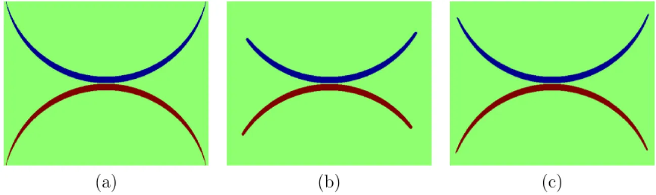
(a) (b) (c)
Figure 2.3: Synthetic example comparing isotropic and anisotropic regularization. (a) original image to be segmented; (b) and (c) three-label segmentation results with isotropic and anisotropic regularization respectively. Anisotropic regularization avoids over-regularization at the tips of the synthetic shape.
segmentation can then be computed from the discontinuity set of u.
2.3.4 Three-label segmentation with anisotropic regularization
The isotropic regularization in model (2.10) treats all directions equally, which is not an ideal choice for long and thin objects like the cartilage. To customize the segmentation model (2.10) for cartilage segmentation, I replace the isotropic regularization term,g, by an anisotropic one
E(u) = Z
Dk
G∇xuk+c|∇lu| dxdl, D = Ω× L,
u∈[0,1], u(x,0) = 0, u(x,3) = 1,
(2.11)
where G is a positive-definite matrix determining the amount of regularization. This avoids over-regularization at the boundaries of the cartilage layers and therefore allows for a more faithful segmentation. Figure 2.3 illustrates the problem with isotropic regu-larization which tends to shrink the segmentation boundary by cutting thin objects short and the benefit from anisotropic regularization. I choose Gas
G=g
Figure 2.4: Difference between isotropic and anisotropic regularization. The black curve is an edge in an image. The regularization is illustrated at a pixel (the dot). The blue circle indicates the isotropic case where regularization is enforced equally in every direction. The red ellipse shows the anisotropic situation where less regularization is applied in the normal direction and more in the tangent direction.
where I is the identity matrix and n is a unit vector indicating the direction of less regularization (the normal direction to the cartilage surface). See Fig. 2.4 for an illus-tration of isotropic versus anisotropic regularization. Since the normal direction to the cartilage surface is not known a-priori, I approximate it by the normal direction to the bone-cartilage interface which can be determined from the segmentations of femur and tibia. The energy functional (2.11) is also convex and therefore a global optimum can also be computed. Again, an iterative gradient descent/ascent scheme is applied for the optimization. See section 2.3.5 for details.
2.3.5 Numerical solution
This section discusses an iterative scheme to optimize (2.11). Solving (2.10) is a special case with G =gI (Iis the identity matrix). I introduce two dual variables p (a vector field) and q (a scalar field) and rewrite (2.11) as
E(u,p, q) = Z
Dh
p,G∇xui+q∇lu dxdl, subject tokpk ≤1, |q| ≤c,
in whichh·,·irepresents inner products. Minimizing (2.11) with respect touis equivalent to minimizing (2.13) with respect tou and maximizing it with respect to p and q.
Taking the variation yields
δE(u,p, q;δu, δp, δq) (2.14)
= ∂
∂
Z
Ω
hp+δp,G∇xu+G∇xδui+ (q+δq)(∇lu+∇lδu) dxdl (2.15) =
Z
Ω
hp,G∇xδui+hδp,G∇xui+q∇lδu+δq∇lu dxdl (2.16) =
Z
Ω
(−div(Gp)− ∇lq)δu+hδp,G∇xui+δq∇lu dxdl (2.17)
The gradient descent/ascent update scheme of (2.13) is
pt=−G∇xu, kpk ≤1 (2.18)
qt=−∇lu, |q| ≤c (2.19)
ut=−divx(Gp)− ∇lq (2.20)
The iterative scheme will lead to a global optimum upon convergence (Appleton and Talbot, 2006) because of the convexity of (2.11). Let S and T denote the source and sink sets: S = Ω× {0},T = Ω× {3}. The region without sources or sinks is denoted as
◦
D = D \(S∪T) = Ω× {1,2}. Zach et al. (2009) proposed to terminate the iterations when the gap between primal energy and dual energy is sufficiently small. The dual energy is computed as
E∗(u) = Z
S
div(Gp) +∇lq dxdl
+ Z
◦ D
min(0,div(Gp) +∇lq)dxdl
(2.21)
increasing after convergence and thresholding of the essentially binary solution u yields an equally globally optimal solution to the original discrete problem.
2.4 Multi-label segmentation
The three-label segmentation (2.10 and 2.11) is a special case of multi-label segmenta-tion. The background label is placed between the two foreground labels so that the same amount (if desired, can also be intentionally different) of spatial regularization is applied to each object with respect to the background. Such symmetric labeling is impossible when the number of labels is greater than three. This section therefore presents a multi-label segmentation method which requires no such symmetric setting and is capable of handling any number of objects.
2.4.1 Limitation of three-label segmentation
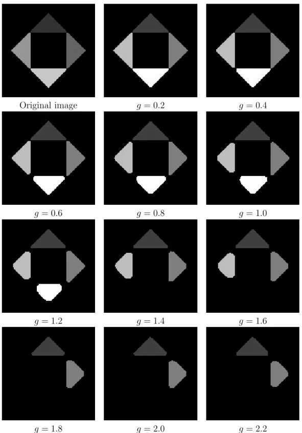
Figure 2.5 shows the regularization issues when applying (2.10) to segment four ob-jects from the background. A symmetric labeling is not possible with more than two objects for model (2.10). Objects with labels closer to the background label get less regularized. In Fig. 2.5, the background is labeled zero so the object with largest label gets the most regularization. As the parameter g in energy (2.10) increases, the objects disappear in the descending order of their labels.
2.4.2 Multi-label segmentation
Original image g = 0.2 g = 0.4
g = 0.6 g = 0.8 g = 1.0
g = 1.2 g = 1.4 g = 1.6
g = 1.8 g = 2.0 g = 2.2
Original image g = 0.2 g = 0.4
g = 0.6 g = 0.8 g = 1.0
g = 1.2 g = 1.4 g = 1.6
g = 1.8 g = 2.0 g = 2.2
Original image g = 0.2 g = 0.4
g = 0.6 g = 0.8 g = 1.0
g = 1.2 g = 1.4 g = 1.6
g = 1.8 g = 2.0 g = 2.2
Original image g = 0.2 g = 0.4
g = 0.6 g = 0.8 g = 1.0
g = 1.2 g = 1.4 g = 1.6
g = 1.8 g = 2.0 g = 2.2
1. The penalty between background and object 4 (whose u = [0,0,0,0,0,1]) will result in penalty 4 as four elements are different. Therefore the spatial regularization depends on the label ordering, meaning a different permutation of labels will result in a different segmentation result. Labels that are farther away from the background will be more smoothed out.
To alleviate the label ordering issue, I propose a novel multi-label segmentation energy functional
E(u) = Z
D
gk∇x∇luk+c|∇lu| dxdl, D= Ω× L subject tou∈[0,1], u(x,0) = 0, u(x, L) = 1.
(2.22)
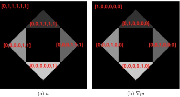
Comparing to (2.10), the regularization term is defined by the spatial gradients of∇lu, rather than u. The reason for such a change can be explained by Fig. 2.1(b) where∇lu
contains a single “1” element for each object. Any two objects differ by 2 when comparing ∇lu. Figure 2.6 demonstrates the advantage of the proposed multi-label segmentation which has no regularization bias therefore is capable of handling any number of objects. The resulting segmentation is independent of label ordering.
The multi-label segmentation problem with anisotropic regularization is formulated as
E(u) = Z
D
kG∇x∇luk+c|∇lu| dxdl, D = Ω× L subject tou∈[0,1], u(x,0) = 0, u(x, L) = 1.
(2.23)
(a) u (b) ∇lu
Figure 2.9: Function u and ∇lu for each object. The labels are assigned as follows. Background: 0, top object: 1, right object: 2, left object: 3, bottom object: 4.
Figure 2.5 shows the problematic regularization of (2.11) when applied to more than three objects. Energy (2.23) overcomes the issue and is therefore capable of dealing with any number of objects. The segmentation results are robust to label ordering.
2.4.3 Numerical solution
This section discusses an iterative scheme to optimize (2.23). Solving (2.22) is a special case with G = gI (I is the identity matrix). I introduce two dual variables p (vector field) and q (scalar field) and rewrite (2.11) as
E(u,p, q) = Z
Dh
p,G∇x∇lui+q∇lu dxdl,
subject to kpk ≤1, |q| ≤c,
(2.24)
in whichh·,·irepresents inner products. Minimizing (2.23) with respect touis equivalent to minimizing (2.24) with respect tou and maximizing it with respect to p and q.
Taking the variation, we have
δE(u,p, q;δu, δp, δq) (2.25)
= ∂
∂
Z
Ωh
p+δp,G∇x∇lu+G∇x∇lδui+ (q+δq)(∇lu+∇lδu) dxdl (2.26) =
Z
Ω
hp,G∇x∇lδui+hδp,G∇x∇lui+q∇lδu+δq∇lu dxdl (2.27) =
Z
Ω
(∇l(div (Gp))− ∇lq)δu+hδp,G∇x∇lui+δq∇lu dxdl (2.28)
The gradient descent/ascent update scheme of (2.24) is
pt=−G∇x∇lu, kpk ≤1 (2.29)
qt=−∇lu, |q| ≤c (2.30)
ut=∇l(div (Gp))− ∇lq (2.31)
◦
D=D\(S∪T) = Ω×{1,2,· · ·, L−1}. Iterations are terminated when the gap between the primal energy (2.11) and the dual energy is sufficiently small. The dual energy is computed as
E∗(u) = Z
S
∇lq− ∇l(div (Gp)) dxdl
+ Z
◦ D
min(0,∇lq− ∇l(div (Gp))) dxdl
(2.32)
The multi-label segmentation can be easily recovered from the discontinuity set of u. Unlike the three-label segmentation, there is no guarantee that solution u is essentially binary after convergence. Thresholding ofudoes not necessarily yield a globally optimal solution to the original discrete problem.
2.5 Conclusion
The main contribution of this chapter is the novel three-label and multi-label seg-mentation framework.
The proposed three-label segmentation framework is general and guarantees separa-tion of the touching objects, e.g., touching bones in Fig. 4.3. By placing the background label in the middle, one can obtain a symmetric labeling with respect to the background. The anisotropic regularization has general applicability for the segmentation of thin ob-jects, e.g., knee cartilage. An important advantage of the segmentation framework is its convexity, which guarantees that a globally optimal solution to the relaxed problem can be computed, which then yields a globally optimal solution to the original problem after thresholding due to its essentially binary property.
compute the globally optimal solution. Unfortunately, the “essentially binary” property is not guaranteed in this case. Therefore, the thresholded solution may not be a globally optimal solution to the discrete formulation, which is a Potts model and known to be NP-hard. However, the solution can be a close approximation to the true optimal solution as it converges to solutions which are close to binary in practice.
CHAPTER 3: AUTOMATIC MULTI-ATLAS-BASED THREE-LABEL CARTILAGE SEGMENTATION
3.1 Introduction
Osteoarthritis (OA) is the most common form of joint disease and a major cause of long-term disability in the United States of America (Woolf and Pfleger, 2003). Cartilage loss is believed to be the dominating factor in OA. As magnetic resonance imaging (MRI) is able to evaluate cartilage volume and thickness and allows reproducible quantification of cartilage morphology (Eckstein et al., 1998, 2006) it is increasingly accepted as a primary method to evaluate progression of OA. An accurate cartilage segmentation from magnetic resonance (MR) knee images is crucial to study OA and would be of particular use for future clinical trials to test so far non-existing disease-progression modifying drugs. Already today, large image databases exist for OA studies which are well suited to design and test automatic cartilage segmentation algorithms capable of processing thousands of images. For example, the Pfizer Longitudinal Study (PLS) dataset (Eckstein et al., 2008) contains 158 subjects, each with five time points. The Osteoarthritis Initiative (OAI) dataset includes 4,796 subjects with multiple time points. Due to the large size of image databases, a fully automatic segmentation and analysis method is essential. In this chapter, I therefore propose a new cartilage segmentation method from knee MR images, which requires no user interaction (besides quality control). The method is a step towards automatic analysis of large OA image databases.
in order to extract the bone-cartilage interface followed by tissue classification. A graph-based simultaneous segmentation of bone and cartilage was developed by Yin et al.
(2010b). Vincent et al. (2010) applied multi-start and hierarchical active appearance modeling to segment cartilage. Texture analysis (Dodin et al., 2010) has also been em-ployed in cartilage segmentation. Seim et al. (2010) utilized prior knowledge on the variation of cartilage thickness. Voxel-based classification approaches have been investi-gated for segmenting multi-contrast MR data by Koo et al. (2009) and Zhang and Lu (2011).
To allow for localized analysis and the suppression of unlikely voxels in a segmentation, introducing a spatial prior is desirable. This can be achieved through an atlas-based analysis method. In particular, multi-atlas segmentation strategies (Rohlfinget al., 2004) have shown to be robust and reliable image segmentation methods. While such methods have been successfully used in brain imaging, they have so far rarely been used for cartilage segmentation. The work by Glocker et al. (2007), which used a statistical shape atlas from a set of pre-aligned knee images, and the work by Tamez-Pe˜na et al.
(2012) using a multi-atlas-based method, are two exceptions. The proposed segmentation method is most closely related to Tamez-Pe˜na et al. (2012) as both methods make use of multi-atlas segmentation strategies. However, I significantly extend the prior work by Tamez-Pe˜naet al. (2012). In particular:
nearest neighbors (kNN) classification and classification by a support vector ma-chine (SVM).
2) I compare different atlas-based segmentation methods: using a single average-shape atlas as well as multiple atlases with various label fusion strategies as segmentation priors.
3) In chapter 4, I perform an extensive validation on over 700 images with varying levels of OA disease progression using data from both the Pfizer Longitudinal Study (PLS) and from SKI10 (Heimannet al., 2010) to compare to existing methods. These contributions are significant as
1) Due to its convexity our segmentation method allows the efficient computation of globally optimal solutions for three segmentation labels, i.e. femoral/tibial carti-lage and background. Furthermore, I demonstrate that anisotropic regularization within this segmentation model is less sensitive to parameter settings than isotropic regularization and yields more accurate cartilage segmentations.
2) I show that using non-local patch-based label fusion from multiple atlases to obtain segmentation priors improves segmentation results significantly over using a single atlas or a local label fusion strategy.
Figure 3.1: Cartilage segmentation pipeline.
Figure 3.1 illustrates the proposed cartilage segmentation method. The method starts with multi-atlas-based bone segmentation to guide the cartilage atlas registration. The cartilage spatial prior is then obtained from either multi-atlas or average-shape-atlas registration. A probabilistic classification is performed to compute local likelihoods. The three-label segmentation makes the final decision from the spatial priors and the local likelihoods jointly, allowing for anisotropic spatial regularization.
3.2 Atlas-based segmentation
An atlas (Aljabar et al., 2009), in the context of atlas-based segmentation, is de-fined as the pairing of an original structural image and the corresponding segmenta-tion. Atlas-based segmentation methods can be categorized into three groups (Iˇsgum
et al., 2009), namely single-atlas-based, average-shape atlas-based, and multi-atlas-based
methods. The work by Glocker et al. (2007) falls into the second group. The work by Tamez-Pe˜na et al. (2012) belongs to the multi-atlas category.
3.3 Multi-atlas-based bone segmentation
The labeling costcin (2.10) for each labellin{FB,BG,TB}(“FB”, “BG” and “TB” denote the femoral bone, the background and the tibial bone respectively) are defined by log-likelihoods for each label given image I at a voxel location x:
c(x, l) = −log(P(l|I(x))) =−log
p(I(x)|l)·P(l)
p(I(x))
. (3.1)
The background label “BG” is placed in the label order between the femur label “FB” and the tibia label “TB” in order to achieve a symmetric formulation.
The likelihood termsp(I(x)|FB) andp(I(x)|TB) are computed from image intensities. Since bones appear dark in T1 weighted MR images, I assume a simple model (3.2) to estimate bone likelihoods,
p(I(x)|FB) =p(I(x)|TB) =exp(−βI(x)), (3.2)
where β is set to 0.02 in our implementation assumingI(x)∈[0,100].
To compute the prior terms p(FB) and p(TB) in (3.1), I employ a multi-atlas reg-istration approach followed by label fusion. Suppose there are N atlases Ai and their bone segmentations areSFB
i and SiTB (i= 1,2, ..., N). Registration from an atlasAi to a
query image I is an affine registrationTaffine
i followed by a B-Spline registration T bspline
i .
Averaging all N propagated atlas labels yields a spatial prior of femur and tibia for the query image:
p(FB) = 1
N N
X
i=1
Tibspline◦Taffine
i ◦SiFB
,
p(TB) = 1
N N
X
i=1
Tibspline◦T affine
i ◦S
TB i
.
Now that I have computed the spatial priors and the local likelihoods, I integrate them into (3.1) and solve (2.10) to obtain the three-label bone segmentation. The bone segmentation will help locate the cartilage in atlas-based cartilage segmentation.
3.4 Probabilistic classification
I use the three-label segmentation with anisotropic regularization for cartilage seg-mentation to account for thin cartilage layers. The labeling cost c for each label l in {FC,BG,TC}(“FC”, “BG” and “TC” denote the femoral cartilage, the background and the tibial cartilage respectively) are defined by log-likelihoods for each label:
c(x, l) =−log(P(l|f(x))) =−log
p(f(x)|l)·p(l)
p(f(x))
, (3.4)
where f(x) denotes a feature vector at a voxel location x. Again the background label “BG” is placed between the femoral cartilage label “FC” and the tibial cartilage label “TC” in order to achieve a symmetric formulation.
An important difference from Folkessonet al.(2007) and Kooet al.(2009) is the prob-abilistic nature of the classification, which allows an easy incorporation of the classifica-tion result into the Bayesian framework. Further, the final segmentaclassifica-tions are generated by a segmentation method with anisotropic regularization, whereas no regularization was used in Folkesson et al. (2007) nor Koo et al. (2009). I demonstrate in chapter 4 that spatial regularization helps improve the segmentation accuracy and anisotropic regular-ization yields better accuracy than isotropic regularregular-ization.
3.4.1 Classification using kNN
I estimate the data likelihoods for femoral and tibial cartilage, p(f(x)|l), of (3.4) by probabilistic kNN classification (Duda et al., 2001). I use a one-versus-other classifica-tion strategy and the expert segmentaclassifica-tions of femoral and tibial cartilage to build the
kNN classifier. Specifically, let “FC” denote the femoral cartilage class, “TC” the tibial cartilage, and “BG” the background class. The training samples of class FC are the voxels labeled as femoral cartilage. Similarly, the training samples of class TC are the voxels labeled as tibial cartilage. The training samples of class BG are the voxels sur-rounding the femoral and tibial cartilage within a specified distance. The outputs of the probabilistic kNN classifier given a query voxel x with its feature vector f(x) are
p(f(x)|FC) = n
FC(f(x))
k ,
p(f(x)|BG) = n
BG(f(x))
k ,
p(f(x)|TC) = n
TC(f(x))
k .
(3.5)
HerenFC,nTC,nBG denote the number of votes for the femoral cartilage, tibial cartilage,
and background class respectively;k is the number of nearest neighbors of concern. Since
training class sizes to balance the three classes.
3.4.2 Classification using an SVM
An alternative approach to compute the local likelihoods is to use a support vec-tor machine (SVM) (Cortes and Vapnik, 1995), which constructs a hyperplane maxi-mally separating classes given a labeled training set. Koo et al. (2009) used two-class SVM to segment cartilage automatically from multi-contrast MR images. I apply LIB-SVM (Chang and Lin, 2011) to perform probabilistic three-class LIB-SVM classification with the features described above. The results are local likelihoods for the background, the femoral and the tibial cartilage, i.e.,p(f(x)|BG), p(f(x)|FC) and p(f(x)|TC). I compare the SVM and thekNN probabilistic classification methods in chapter 4.
3.5 Average-shape-atlas-based cartilage segmentation
This section discusses how to build a probabilistic bone and cartilage atlas by av-eraging registered expert segmentations and computing the cartilage spatial priors by registration of the atlas. The atlas within this section captures the spatial relationships between the bone and the cartilage.
Suppose there are N images with expert segmentations. One can pick the segmenta-tion of one image as the reference to bring all the segmentasegmenta-tions to the same posisegmenta-tion. Specifically, I register the femur segmentationSFB
i (i= 1,2, ..., N) and the tibial
segmen-tation STB
i (i = 1,2, ..., N) to the reference femur and tibia segmentations with affine
transforms TFB
i and TiTB respectively. The femoral and tibial cartilage segmentations SFC
(including AFB
avg,ATBavg, AFCavg and ATCavg) is computed by
AFB avg = 1 N N X i=1 TFB
i ◦S
FB i , ATB avg = 1 N N X i=1 TTB
i ◦SiTB
, AFC avg = 1 N N X i=1 TFB
i ◦SiFC
,
ATCavg =
1
N N
X
i=1
TiTB◦S TC i
.
(3.6)
Given a query image I, I have computed the bone segmentation SFB and STB from
section 3.3. The atlas femur AFB and tibia AFB are registered to the segmentation of
femurSFB and tibiaSTB with affine transforms TFB and TTB. The spatial prior for each
cartilage is then computed by propagating each cartilage atlas with the corresponding transform,
p(FC) =TFB
◦AFC
avg,
p(TC) =TTB◦ATCavg,
p(BG) = 1−p(FC)−p(TC).
(3.7)
These spatial priors and the local likelihoods from section 3.4 are integrated into (3.4) and the cartilage segmentation is obtained by optimizing the three-label segmentation energy with anisotropic regularization (2.11).
3.6 Multi-atlas-based cartilage segmentation
described in section 3.5. Each atlas is an individual expert bone and cartilage segmen-tation in this section. Three popular label fusion methods are discussed in this section, i.e., majority voting, locally-weighted and non-local patch-based fusion.
Suppose there are N atlases Ai including their femur segmentations SFB
i , tibia
seg-mentations STB
i , femoral cartilage segmentations SiFC and tibial cartilage segmentations STC
i (i= 1,2, ..., N). For a query imageI, we have the bone segmentation SFB and STB
from section 3.3.
The atlas bone segmentations SFB
i and SiTB are registered to the bone segmentations SFB and STB of the query image separately by affine transforms TFB
i and TiTB.
One can simply take the average of the registered cartilage atlas segmentations to compute the spatial priors, which is majority voting Rohlfing et al.(2004) label fusion:
p(FC) = 1
N N
X
i=1
TFB
i ◦S
FC i
,
p(TC) = 1
N N
X
i=1
TTB
i ◦S
TC i
.
(3.8)
One can also apply a locally-weighted label fusion strategy (Iˇsgumet al., 2009), which was shown to yield a better segmentation accuracy than a majority voting strategy. In this case, I choose to favor the atlases which locally agree better with the cartilage likelihoodsp(f(x)|FC) andp(f(x)|TC) from the probabilistic classification in section 3.4. The spatially varying weighting functions λFC
i for the femoral cartilage and λTCi for the
tibial cartilage are calculated as
λFC i (x) =
1
α|TFB
i ◦SiFC−p(f(x)|FC)|+
,
λTCi (x) =
1
α|TTB
i ◦SiTC−p(f(x)|TC)|+
,
(3.9)
my implementation. The spatial prior for each cartilage is then the weighted average of the propagated atlas cartilage segmentations
p(FC) =
N X i=1 λFC i PN
i=1λ
FC i
TiFB◦S FC i
,
p(TC) =
N X i=1 λTC i PN
i=1λ
TC i
TTB
i ◦S
TC i
.
(3.10)
Recently, non-local patch-based label fusion techniques have been proposed by Coup´e
et al.(2011) and Rousseauet al.(2011). Instead of deciding the label from the same voxel
location in each propagated atlas, these methods obtain a label using the surrounding patches in a predefined neighborhood across the training atlases. Weights are assigned to these patches according to the distances between the target patch and the selected patches. This allows local robustness to registration error.
LetpFC(x) andpTC(x), respectively, denote the spatial prior of femoral cartilage (i.e., p(FC)) and tibial cartilage, (i.e. p(TC)) at voxel x. I calculate the probabilities by weighted averages of the propagated labels in a pre-specified search neighborhoodN(x) across N warped atlases. The weights are determined by local patch similarities. For simplicity, let ˜SFC
i =TiFB◦SiFC and ˜IiFC =TiFB ◦Ii. Here, i is the atlas index, running
from 1 toN, SFC
i refers to the femoral cartilage segmentation of the i-th atlas, and Ii is
the i-th atlas appearance. For the femoral cartilage, the probability is computed as
pFC(x) =
N
P
i=1
P
y∈N(x)
wFC(x,y) ˜SFC
i (y)
N
P
i=1
P
y∈N(x)
wFC(x,y)
, (3.11)
wFC(x,y) = exp
P
x0∈P(x) y0∈P(y)
I(x0)−I˜FC
i (y
0)2 hFC(x)
where x0 is a voxel in the patch P(x) centered at x (similarly y0 a voxel in the patch P(y) centered at y) andhFC(x) is defined by
hFC(x) = min 1≤i≤N
y∈N(x)
X
x0∈P(x)
y0∈P(y)
I(x0)−I˜FC
i (y
0
)
2
+. (3.13)
Substitute “FB” with “TB” and “FC” with “TC” in superscripts of the equations above for the calculation of pTC(x).
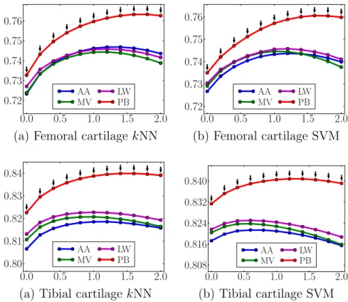
The three label fusion strategies, namely majority voting, locally-weighted and non-local patch-based fusion, are compared in chapter 4. The non-non-local patch-based method is shown to result in the best average segmentation accuracy.
These spatial priors and the local likelihoods from section 3.4 are integrated into (3.4) and the cartilage segmentation is obtained by optimizing the three-label segmentation energy with anisotropic regularization (2.11).
3.7 Overall segmentation pipeline
The automatic cartilage segmentation requires expert segmentations of femur, tibia, femoral and tibial cartilage on a set of training images. Given a query knee image, I first correct the MRI bias field (Sledet al., 1998), scale image intensities to a common range, and then perform edge-preserving smoothing using curvature flow (Sethian, 1999).
Once I have the bone segmentation, I perform the probabilistic classification (kNN or SVM) of knee cartilage in the joint region. The spatial priors for the cartilage can be obtained through registration of an average bone and cartilage atlas, which requires only one registration, or through a multi-atlas registration of cartilage, which needs a number of registrations. If a multi-atlas-based method is chosen, propagated atlas labels are fused (using majority voting, locally-weighted or non-local patch-based label fusion) to obtain the spatial priors. The normal direction n in (2.12) is computed by taking the gradient of the diffusion smoothed three-label bone segmentation result within the joint area. Finally, the local likelihoods and the spatial priors are integrated into the three-label segmentation to generate the cartilage segmentation.
3.8 Conclusion
The major contribution of this chapter is the fully-automatic cartilage segmentation method that incorporates local classification (from image appearance) and shape infor-mation (from atlas registration) into the three-label segmentation framework discussed in chapter 2.
I used a multi-atlas-based bone segmentation to guide the registration of a cartilage atlas. I obtained cartilage segmentation using an average shape atlas or multiple atlases with various label fusion techniques to obtain spatial cartilage priors within the three-label segmentation framework, which incorporates anisotropic regularization to improve segmentation performance (shown in chapter 4) for the thin femoral and tibial cartilage layers.
The overall pipeline is fully-automatic (besides quality control), which enables the method to be applied to large image databases. The robustness due to multi-atlas-based strategies also makes the proposed method appropriate for large datasets.
the PLS dataset (Eckstein et al., 2008) and SKI10 dataset (Heimann et al., 2010), on which I compare the proposed method to existing ones quantitatively.
CHAPTER 4: VALIDATION OF CARTILAGE SEGMENTATION 4.1 Introduction
This chapter presents the validations results of the proposed cartilage segmentation method in chapter 3 on two datasets, PLS (Eckstein et al., 2008) and SKI10 (Heimann
et al., 2010).
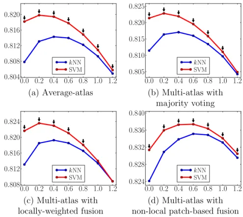
The main validation is performed on the PLS dataset. I compare different atlas choices for cartilage segmentation, namely average-shape-atlas and multi-atlas with various label fusion strategies (majority voting, locally-weighted voting and patch-based label fusion). I also compare the two probabilistic tissue classification, i.e.,kNN and SVM. The impact of isotropic and anisotropic regularization is also studied.
To compare to other existing methods quantitatively, I test the proposed method on a publicly available dataset, SKI10.
4.2 Data description
The main dataset is the PLS dataset, containing 706 T1-weighted (3D oblique coronal spoiled gradient recalled) images for 155 subjects, imaged at baseline, 3, 6, 12, and 24 months at a resolution of 1.00×0.31×0.31mm3. Some subjects have missing scans. The
Kellgren-Lawrence grades (KLG) (Kellgren and Lawrence, 1957) were determined for all subjects from the baseline scans, classifying 82 as normal control subjects (KLG0), 40 as KLG2 and 33 as KLG3.