TRACKING THE SOURCES AND FATES OF FLUORESCENT ORGANIC MATTER IN THE EUTROPHIC NEUSE RIVER ESTUARY, NORTH CAROLINA
Alexandria G. Hounshell
A dissertation submitted to the faculty at the University of North Carolina at Chapel Hill in partial fulfillment of the requirements for the degree of Doctor of Philosophy in the Department
of Marine Sciences.
Chapel Hill 2019
© 2019
ABSTRACT
Alexandria G. Hounshell: Tracking the sources and fates of fluorescent organic matter in the eutrophic Neuse River Estuary, North Carolina
(Under the direction of Hans W. Paerl)
Eutrophication is defined as ‘an increase in the rate of supply of organic matter (OM) to an ecosystem’. In estuaries, this can take two forms: an increase in allochthonous and an increase in autochthonous OM. The goal of this dissertation was to use spectrofluorometry, as excitation emission matrices (EEMs), and other measures of OM quantity and quality, to constrain the OM pool in the Neuse River Estuary (NRE) and to assess how climate change and human activities in the watershed are altering the quantity and quality of OM.
EEMs can be coupled with the statistical decomposition technique, parallel factor analysis (PARAFAC), to identify broad classes of fluorescent OM (FOM). The first chapter assessed the use of PARAFAC as applied to fluorescent dissolved OM (FDOM) and base extracted
fluorescent particulate OM (BEFPOM) and determined the dominate sources of these two pools were different. The second chapter used multivariate statistics to identify sources of FOM. Results suggest the FDOM pool is composed of terrestrial, humic-like OM while the FPOM pool contains terrestrial, humic-like and autochthonous OM.
ACKNOWLEDGEMENTS
TABLE OF CONTENTS
LIST OF TABLES ... xi
LIST OF FIGURES ... xiii
LIST OF ABBREVIATIONS AND SYMBOLS ... xvi
CHAPTER 1: INTRODUCTION AND MOTIVATION ... 1
REFERENCES ... 9
CHAPTER 2: USING EXCITATION EMISSION MATRICES COUPLED WITH PARALLEL FACTOR ANALYSIS (EEM-PARAFAC) TO CHARACTERIZE FLUORESCENT ORGANIC MATTER SIGNATURES, SOURCES AND TRANSFORMATIONS IN THE NEUSE RIVER ESTUARY, NORTH CAROLINA ... 13
1. Summary ... 13
2. Introduction ... 14
3. Methods... 18
3.1 Sample collection ... 18
3.2 PARAFAC modeling ... 22
3.3 Experimental bioassays ... 23
3.4 Estuarine FDOM signal identification ... 24
3.5 FluorMod ... 25
4. Results and Discussion ... 26
4.1 Environmental parameters ... 26
4.2 FDOM PARAFAC modeling ... 29
4.4 FDOM+BEFPOM PARAFAC modeling ... 37
4.5 PARAFAC model comparisons ... 41
4.6 FluorMod estuarine signal ... 43
4.7 Application of FluorMod ... 53
5. Conclusions ... 58
REFERENCES ... 61
CHAPTER 3: SPATIAL AND TEMPORAL DISTRIBUTION OF FLUORESCENT ORGANIC MATTER IN THE NEUSE RIVER ESTUARY, NORTH CAROLINA ... 67
1. Summary ... 67
2. Introduction ... 68
3. Materials and Methods ... 71
3.1 Study site and sampling methods ... 71
3.2 Organic matter analysis ... 73
3.3 Chlorophyll a analysis ... 76
3.4 River discharge and meteorological data ... 76
4 Results and Discussion ... 78
4.1 Environmental and organic matter parameters ... 78
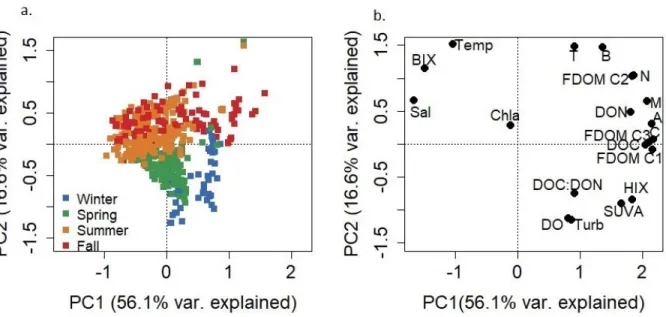
4.2 Multivariate statistics ... 82
4.3 Principal component analysis ... 87
5 Conclusions: Implications for organic matter dynamics in estuarine environments ... 97
CHAPTER 4: UNDERSTANDING ORGANIC MATTER SOURCE AND SINK TERMS IN A HYDROLOGICALLY VARIABLE ESTUARY USING A NON-STEADY STATE BOX MODEL APPROACH ... 104
3.2 DOM load ... 111
3.3 Volume weighted DOM concentrations ... 115
3.4 DOM source & sink term ... 115
3.5 Estimates of biological processes ... 116
4. Results ... 118
4.1 Discrete discharge events ... 118
4.2 DOM load ... 118
4.3 Volume weighted DOM concentrations ... 119
4.4 Estuarine flow ... 121
4.5 Estimates of biological processes ... 122
5. Discussion ... 125
5.1 DOM processes in the NRE... 128
5.2 Pulse-Shunt concept in estuarine ecosystems ... 130
6. Conclusion ... 133
REFERENCES ... 135
CHAPTER 5: STIMULATION OF PHYTOPLANKTON PRODUCTION BY ANTHROPOGENIC DISSOLVED ORGANIC NITROGEN IN A COASTAL PLAIN ESTUARY ... 141
1. Summary ... 141
2. Introduction ... 142
3. Materials and Methods ... 143
3.1 Site description ... 143
3.2 Experimental Design ... 144
3.3 Optical analyses ... 148
3.4 Phytoplankton biomass, primary productivity, and bacterial productivity ... 150
3.6 Statistical analysis... 150
4. Results and Discussion ... 151
4.1 Phytoplankton growth response ... 151
4.2 DOM characteristics: EEM-PARAFAC FDOM Components, DOC, and DON ... 154
4.3 Source EEMs ... 155
4.4 Residual PARAFAC model ... 158
5. Conclusions: Implications for estuarine management ... 162
REFERENCES ... 164
CHAPTER 6: CONCLUSIONS ... 169
REFERENCES ... 175
APPENDIX 2: CHAPTER 2 SUPPLEMENTARY INFORMATION ... 177
Appendix 2.1 Environmental Parameters... 177
Appendix 2.2. FDOM Model: ... 179
Appendix 2.3. BEFPOM Model: ... 184
Appendix 2.4. FDOM+BEFPOM Model: ... 190
Appendix 2.5. Estuarine signal: ... 201
Appendix 2.6. Application of FluorMod: ... 208
REFERENCES ... 213
APPENDIX 3: CHAPTER 3 SUPPLEMENTARY INFORMATION ... 214
Appendix 3.1: Wind speed, gusts, and direction for the Neuse River Estuary ... 214
Appendix 3.2: Correlations for the Environmental, DOM, and POM data sets ... 215
Appendix 3.3: Principal component analysis results plotted by depth and location ... 219
Appendix 3.6: Co-inertia Analysis results for Environmental data vs. DOM and POM data
matrices ... 231
APPENDIX 4: CHAPTER 4 SUPPLEMENTARY INFORMATION ... 235
Appendix 4.1. Absorbance measurements ... 235
Appendix 4.2: ModMon sampling dates and C-parameters collected ... 236
Appendix 4.3. NRE Volumes and surface area ... 237
Appendix 4.4: Salinity, DOC, and a350 box models: ... 238
4.4.1: Salinity box model:... 238
4.4.2 DOC and a350 box model: ... 242
Appendix 4.5. Estimating the 95% confidence intervals ... 243
Appendix 4.6. Location of rainfall in the Neuse River watershed ... 244
Appendix 4.7. Estimate of pore water DOC stock in the NRE ... 253
Appendix 4.8. Volume weighted parameters ... 254
Appendix 4.9. NRE wind conditions ... 255
REFERENCES ... 256
APPENDIX 5: CHAPTER 5 SUPPLEMENTARY INFORMATION ... 257
LIST OF TABLES
Table 2.1. Experimental bioassay treatments used to isolate the estuarine FDOM
signal. ... 24
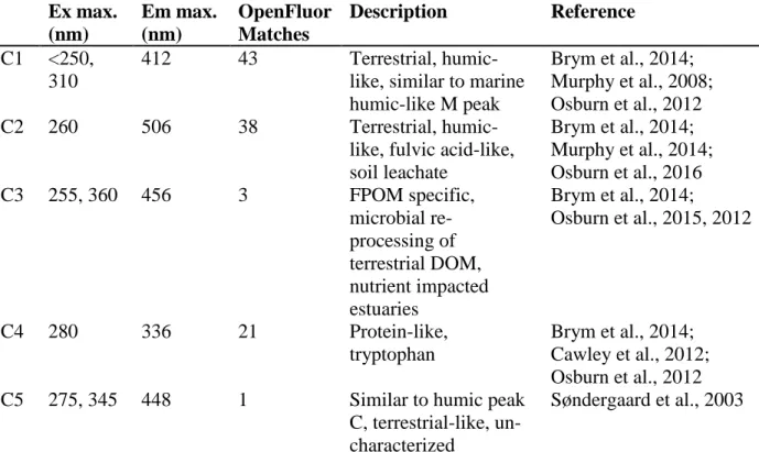
Table 2.2. OpenFluor matches for the 3-component FDOM model ... 30
Table 2.3. OpenFluor matches for the 5-component FPOM model. ... 34
Table 2.4. OpenFluor matches for the 5-component FDOM+FPOM model ... 39
Table 2.5. Model comparisons between the three PARAFAC models generated for samples collected from the NRE ... 42
Table 2.6. OpenFluor matches for the 1-component PARAFAC model developed on experimental bioassay FDOM samples ... 46
Table 2.7. OpenFluor matches for the 2-component PARAFAC model developed on experimental bioassay FDOM samples from July 2017 ... 48
Table 2.8. Results from applying PARAFAC models to various subsets of subtracted samples collected from the experimental bioassays ... 49
Table 3.1. Range of HIX and BIX values and the associated OM characterization ... 75
Table 3.2. Previously identified and characterized fluorescence peaks from the literature used in the peak-picking method ... 75
Table 3.3. Parameters that are not correlative (r2 < 0.80) ... 84
Table 3.4. Pearson r2 for all parameters (environmental, DOM, and POM) used for subsequent multivariate analyses. ... 86
Table 3.5. RDA results for DOM and POM data ... 94
Table 4.1. Discharge values for the seven discrete discharge events ... 113
Table 4.2. Summary of C fluxes as averaged over each discrete discharge event ... 127
Table 5.2. Results from the RM-ANOVA conducted on the coupled DOM addition and inorganic nutrient addition treatments for Chl a and primary
LIST OF FIGURES
Figure 2.1. Map of the NRE located in eastern NC ... 20 Figure 2.2. Boxplots of various chemical and biological (a. DOC, b. DON, c.
POC, d. PN, e. Chl a) parameters plotted down estuary by station ... 28 Figure 2.3. Model components (C1-C3) for the 3-component FDOM model. ... 29 Figure 2.4. Boxplots of each of the three identified FDOM PARAFAC
components plotted by station for all time points and depths ... 31 Figure 2.5. PCA results as applied to DOM parameters, including the
3-components identified in the FDOM model ... 32 Figure 2.6. 5-component PARAFAC model developed on collected BEFPOM
samples ... 34 Figure 2.7. Boxplots of the 5 BEFPOM components plotted down estuary by
station ... 36 Figure 2.8. PCA results for FPOM parameters ... 37 Figure 2.9. 5-component PARAFAC model developed for FDOM+BEFPOM
samples ... 38 Figure 2.10. PCA results as applied to components from all three models
(FDOM, BEFPOM, FDOM+BEFPOM applied to FDOM samples,
FDOM+BEFPOM applied to FPOM samples) ... 43 Figure 2.11. Plots of Chl a through time for each of the experimental bioassays
used to identify an FDOM estuarine processing signal ... 45 Figure 2.12. Estuarine processing signal identified from samples collected
during all of the experimental bioassays ... 46 Figure 2.13. 2-component model identified from the July 2017 experiment ... 48 Figure 2.14. Absorbance at 350 nm (a350) plotted for each treatment and
Figure 2.17. FluorMod 9-component model as applied to an FDOM sample
collected on 04-06-16 from Station 100 bottom ... 56
Figure 2.18. Estuarine processing signal plotted down estuary as applied to residual samples after application of FluorMod ... 56
Figure 2.19. Estuarine processing signal applied to sample residuals after the application of the FDOM 3-component model developed for the NRE. ... 57
Figure 3.1. Map of the NRE located in Eastern NC ... 72
Figure 3.2. Salinity and Chl a plotted seasonally for all time points, stations, and depths collected during the sampling period ... 79
Figure 3.3. a. DOC (mg L-1), b. POC (mg L-1), c. DOM HIX, and d. POM HIX plotted seasonally for all collected time points, stations, and depths ... 80
Figure 3.4. Comparison between salinity and DOM parameters averaged monthly from 2010-2011 (Dixon et al., 2014) compared to 2015-2016 (this study). ... 82
Figure 3.5. PCA results for the a. Environmental, b. DOM, and c. POM data sets ... 89
Figure 3.6. PCA results including wind direction and speed data ... 92
Figure 3.7. RDA results plotted for a. DOM and b. POM ... 94
Figure 3.8. CoIA results for DOM vs. POM parameters. ... 97
Figure 4.1. Map of the NRE located in Eastern NC ... 109
Figure 4.2. Daily discharge (black lines) obtained from Ft. Barnwell USGS gaging station plotted for the study period ... 112
Figure 4.3. a. Head of estuary [DOC] (mg L-1) and b. a350 (m-1) plotted against discharge (m3 s-1). c. DOC load (kg d-1) plotted against a350 load (m2 d-1). ... 119
Figure 4.4. a. Volume weighted [DOC] (mg L-1) plotted in the black circles and volume weighted a350 (m-1) plotted in white circles. b. Volume weighted salinity ... 120
Figure 4.5. a. [DOC] (mg L-1) and b. a350 (m-1) plotted for station 160 versus estuarine flow. c. Estuarine flow (m3 s-1) as calculated for station 160. ... 122
Figure 4.7. a. DOC source & sink term (kg d-1) plotted against estimates of DOC production by PP (kg d-1). b. DOC source & sink term (kg d-1) plotted
against a350 source & sink term ... 129 Figure 5.1. Chl a (left) and primary productivity (Prim. Prod.) (right) plotted for
each coupled DOM addition treatment ...152 Figure 5.2. Sample EEM (top), PARAFAC modeled EEM (middle), and residual
EEM (bottom) for DOM addition sources ...157 Figure 5.3. PARAFAC component unique to the chicken litter leachate (June
2014, October 2014) treatment samples (left) and the Ex and Em spectra
(right) ...159 Figure 5.4. Residual PARAFAC component applied to bioassay fluorescence
samples plotted through the bioassay for both the respective inorganic
LIST OF ABBREVIATIONS AND SYMBOLS
a254 Absorbance at 254 nm
a350 Absorbance at 350 nm
BEFPOM Base extracted fluorescent particulate organic matter
BIX Biological Index
C Carbon
CDOM Colored Dissolved Organic Matter
Chl a Chlorophyll-a
CO2 Carbon Dioxide
CoIA Co-Inertia Analysis
DIN Dissolved Inorganic Nitrogen
DO Dissolved Oxygen
DOC Dissolved Organic Carbon
DOM Dissolved Organic Matter
DON Dissolved Organic Nitrogen
EEMs Excitation Emission Matrices
EWE Extreme weather event
FDOM Fluorescent Dissolved Organic Matter
FI Fluorescent Intensity
FOM Fluorescent Organic Matter
FPOM Fluorescent Particulate Organic Matter
HIX Humification Index
ModMon Neuse River Estuary Modeling and Monitoring Project
N Nitrogen
NaOH Sodium hydroxide
NH4+ Ammonium
nMDS Non-metric multidimensional scaling
NO2- Nitrite
NO3- Nitrate
NR Neuse River
NRE Neuse River Estuary
OC Organic Carbon
OM Organic Matter
ON Organic Nitrogen
P Phosphorus
PAR Photosynthetically Active Radiation
PARAFAC Parallel Factor Analysis
PCA Principal Component Analysis
pCO2 Partial pressure of Carbon Dioxide
PN Particulate Nitrogen
PO43- Phosphate
PS Pamlico Sound
PSC Pulse Shunt Concept
PSU Practical Salinity Units
Q Discharge
Q.S.E. Quinine Sulfate Equivalents
Q.S.U. Quinine Sulfate Units
RDA Redundancy Analysis
RM-ANOVA Repeated Measures Analysis of Variance
Sal Salinity
SUVA254 Specific Absorption at 254 nm
TCC Tucker's Congruence Coefficient
TDN Total Dissolved Nitrogen
tDOC Terrestrial Dissolved Organic Carbon
Temp Temperature
TMDLs Total Maximum Daily Loads
TOC Total Organic Carbon
Turb Turbidity
WRTDS Weighted Regression on Time, Discharge, and Season
CHAPTER 1:INTRODUCTION AND MOTIVATION
Organic matter (OM) plays an important role in regulating key processes in aquatic systems including: light availability (Osburn et al., 2009), the complexation and transport of metals (Bergamaschi et al., 2012), transport of pollutants (Ripszam et al., 2015), a carbon (C) substrate for microbial respiration (Moran et al., 2000) and a nutrient source, as either nitrogen, N or phosphorus, P, to primary production (Boyer et al., 2006; Bronk et al., 2007). Additionally, OM plays an important role in controlling the eutrophication status of an ecosystem. Eutrophication, as defined by Nixon, 1995, is ‘an increase in the rate of supply of OM to an ecosystem’. In coastal, aquatic ecosystems, this can either be in the form of terrestrial OM flushed into the system from the watershed (i.e., allochthonous OM) or from autochthonous OM produced when phytoplankton convert inorganic nutrients (as N and P) to biomass in situ (Nixon, 1995). Both pathways of eutrophication can lead to negative impacts on affected coastal ecosystems, including bottom water hypoxia/anoxia, fish kills, habitat degradation, and the formation of nuisance or harmful algal blooms, all of which disrupt ecosystem function and can lead to cascading negative impacts up the food web (Cloern, 2001; Nixon, 1995).
Eutrophication has been a widely recognized problem in coastal ecosystems, including estuaries, for several decades and efforts have been enacted in an attempt to reduce
point-sources (i.e., wastewater treatment facilities – WWTF; agricultural operations; industrial inputs) historically high in dissolved inorganic N (Lebo et al., 2012; Paerl et al., 2004). While these efforts have led to a reduction in inorganic N loading, there has been a reported increase in organic N (ON) to riverine and estuarine ecosystems (Pellerin et al., 2006, Lebo et al., 2012, Harrington and Bowen, 2017), including in response to expected increases in precipitation due to climate change (Gabriel et al., 2015). Additionally, chlorophyll a (Chl a) concentrations, used as a proxy for phytoplankton biomass and as a measure for the effectiveness of enacted nutrient reductions, have not been shown to decrease in response to the decreasing N loading in many of these systems (Cloern, 2001; Paerl et al., 2010, Lebo et al., 2012, Keith, 2014).
Terrestrial OM loading is also an important factor in terms of eutrophication, either as an increase in the rate of supply of terrestrial OM to the system or as a nutrient source, specifically as a N-source, supporting phytoplankton growth (Berman and Bronk, 2003; Bronk et al., 2007; Eom et al., 2017; Seitzinger et al., 2002). Historically, identifying and tracking OM, both as terrestrial and autochthonous OM sources, has been time consuming and expensive. These constraints limited the number of samples that could be collected and used to assess the temporal and spatial variability of OM in an ecosystem, making it difficult to resolve the sources, fates, and role OM plays in eutrophication and its potential role in stimulating phytoplankton growth. More recently, the use of spectrofluorometry (i.e., fluorescence) in conjunction with bulk OM measurements, have been used to rapidly and broadly characterize the OM pool in a variety of aquatic ecosystems, including estuaries (Brym et al., 2014; Coble, 1996; Jaffé et al., 2014; Markager et al., 2011; Osburn et al., 2012; Stedmon and Markager, 2005).
(FPOM), as well as assess the sources and fates of broad classes of fluorescent OM (FOM) in situ. Spatially, the sources of OM to many estuaries transition from allochthonous, terrestrial
sources in the upper estuary where riverine loading is the main driver of OM to more
autochthonous sources of OM produced in situ (i.e., phytoplankton and microbial production) (Canuel and Hardison, 2016; Markager et al., 2011). The transition from allochthonous in the upper estuary to autochthonous OM in the mid to lower estuary is due to a combination of physical, chemical, and biological processes including: conservative mixing as the highly concentrated riverine water mixes with less concentrated marine water (Markager et al., 2011); photochemical and microbial degradation which transforms and removes allochthonous and autochthonous sources of OM (McCallister et al., 2006; Osburn et al., 2009; Stedmon and Markager, 2005); and production and consumption of OM in situ by phytoplankton and microbial assemblages (McCallister et al., 2006). Temporally, the sources and fates of OM in estuaries are highly variable and are largely driven by seasonal changes occurring in both the watershed (i.e., hydrologic flow path, leaf litter fall, seasonal precipitation patterns) (Singh et al., 2014) and in the estuary (i.e., photochemical and microbial degradation, phytoplankton
production) (Canuel and Hardison, 2016). However, in addition to seasonal changes, temporal OM changes are also heavily driven by physical conditions affecting the estuary, including riverine discharge and wind-driven sediment resuspension events (Canuel and Hardison, 2016; Crosswell et al., 2017; Dixon et al., 2014; Osburn et al., 2012).
and POM pools, respectively (Canuel and Hardison, 2016; McCallister et al., 2006; Osburn et al., 2012). The DOM pool is mainly composed of allochthonous and bacterially degraded DOM while the POM pool is generally thought to be comprised of both allochthonous sources and autochthonous POM generated by phytoplankton growth in situ (McCallister et al., 2006). The sources, molecular size, and chemical structure of the DOM and POM pools influence its bio-reactivity and ultimate fate in estuarine environments (McCallister et al., 2006; Raymond and Bauer, 2001). McCallister et al., (2006) hypothesized the highly terrestrial and bacterial nature of the DOM pool in estuaries was due to the rapid conversion of autochthonous DOM by bacteria in situ while the autochthonous nature of POM is allowed to persist due to its lower bio-reactivity.
Studies have also demonstrated transformations between the POM and DOM pool (Asmala et al., 2018), especially along the estuarine turbidity maximum where POM concentrations are high and sediment resuspension events are common (Canuel and Hardison, 2016). However, few studies have simultaneously assessed the quality and quantity of both DOM and POM spatially and temporally in estuarine ecosystems (McCallister et al., 2006; Osburn et al., 2012).
The goal of this study was to better understand the similarities, differences, and linkages between the sources and transformations of the FDOM and FPOM pools in estuarine
environments and to provide a baseline and understanding for how the FOM pool in estuaries is changing due to climatic and anthropogenic pressures. This includes how an increasing
autochthonous FOM in a eutrophic estuarine environment, the Neuse River Estuary (NRE), North Carolina, USA, including following an extreme precipitation event. The research will further our understanding of the transport of and role terrestrial and autochthonous OM plays in stimulating and sustaining eutrophication and its negative impacts in coastal, estuarine systems.
The first part of this study, chapter 2 focused on the use of spectrofluorometry as EEMs coupled with PARAFAC (EEM-PARAFAC) to assess the sources and transformations of both the FDOM and base extracted FPOM (BEFPOM) pools simultaneously, in the NRE. The goal of this chapter was to assess the use and utility of PARAFAC modeling to understand differences in the FDOM and BEFPOM pools in estuarine environments as well as to identify and track an estuarine FDOM signal (i.e., phytoplankton and microbial production plus photochemical and microbial degradation of FDOM) in situ. Ultimately, the identified estuarine FDOM signal could be incorporated into an existing FDOM source-based PARAFAC model, FluorMod (Osburn et al., 2016), and used to track watershed and autochthonous sources of FDOM through a dynamic, eutrophic estuary. Results from this chapter highlight the differences, in terms of dominate sources, of the FDOM and BEFPOM pools. Additionally, an estuarine FDOM signal was identified using experimental bioassays; however, the signal was not identified in FDOM samples collected from the NRE due to the overwhelming fluorescence intensity of terrestrial FDOM in situ.
of DOM and POM in the NRE, but also to identify potential linkages and transformations between the DOM and POM pools in situ. Results from this chapter demonstrate the utility of using multivariate techniques originally designed for analysis of ecological data sets, as applied to data sets of environmental parameters, DOM, and POM to assess the relationships and drivers between these three sets of measurements.
While chapters 2 and 3 serve as a baseline for understanding the current dynamics of FDOM and FPOM in eutrophic estuaries, Chapter 4 assessed how DOM dynamics in the NRE may change under increasing frequency of extreme precipitation events due to climate change. A non-steady state box model approach was used to constrain flow into and out of the marine end member and to calculate DOC and CDOM (as absorbance measured at 350 nm, a350) source and sink terms under varying riverine discharge conditions, spanning from baseflow to extreme flow (4th to 99th flow quantiles, respectively). The study also incorporated measurements of CO2 efflux and phytoplankton primary production to provide linkages between observed DOC dynamics and both potential DOC degradation and production processes, as respiration of DOC to CO2 and primary production, in the estuary. The variability of the resolved values from the salinity and OM box models was high, indicating the coarse spatial and temporal scale used for both the estuarine monitoring effort and box model approach was not able to accurately constrain in situ dynamics in this estuary. Following extreme riverine discharge events, however, results
Finally, chapter 5 focused on the role watershed FDOM sources may play as a nutrient source, specifically as an N (DON) source, for stimulating phytoplankton growth in the NRE. Using a series of experimental watershed DON addition bioassays, I determined chicken litter leachate was capable of stimulating phytoplankton growth in excess of that stimulated by the inorganic nutrients contained in this source alone. Using the EEM-PARAFAC technique, I identified a fluorescence signal which may be responsible for stimulating this excess growth. I demonstrated that other watershed sources of DON (WWTF effluent, turkey litter leachate, concentrated river DON) do not stimulate phytoplankton growth.
Taken collectively, overarching results from this study suggest the FOM pool in the NRE was overwhelmingly dominated by terrestrial FDOM. The DOC pool was 85% of the total organic C (TOC) while the POC pool represented 15% of TOC, as was indicated by bulk concentrations. In terms of OM quality, FDOM results suggest the FDOM pool was almost completely dominated by terrestrial, humic-like FOM (93% allochthonous FDOM; 7%
autochthonous FDOM). While FPOM results did indicate the FPOM pool contains compounds from both allochthonous (37%) and autochthonous (63%) sources, the relative amounts of autochthonous FPOM compared to the overall FOM pool, were small (~ 4%). The dominance of terrestrial fluorescent signals, particularly in the FDOM pool, made it difficult to identify
and can be subtracted from measured EEMs collected in aquatic ecosystems, it may be possible to capture these same biological signals in situ (Murphy et al., 2018).
Results from the last two chapters demonstrated that the OM pool, specifically the DOM pool, in the NRE is changing. This includes changes associated with the increase in recent extreme precipitation events, as predicted in response to climate change (Bender et al., 2009; Janssen et al., 2016), which were shown to alter how the estuary exports DOC to the coastal end member, as well as changes to the sources of watershed nutrients, as DON. Overall, within the time scale of exposure (days to several weeks), sources of watershed DON generally do not appear to stimulate growth of phytoplankton and microbial assemblages in estuarine
REFERENCES
Asmala, E., Haraguchi, L., Markager, S., Massicotte, P., Riemann, B., Staehr, P.A., Carstensen, J., 2018. Eutrophication Leads to Accumulation of Recalcitrant Autochthonous Organic Matter in Coastal Environment. Global Biogeochemical Cycles 32, 1673–1687.
https://doi.org/10.1029/2017GB005848
Bender, M.A., Knutson, T.R., Tuleya, R.E., Sirutis, J.J., Vecchi, G.A., Garner, S.T., Held, I.M., 2009. Modeled Impact of Anthropogenic Atlantic Hurricanes. Science 327, 454–458. Bergamaschi, B.A., Krabbenhoft, D.P., Aiken, G.R., Patino, E., Rumbold, D.G., Orem, W.H.,
2012. Tidally Driven Export of Dissolved Organic Carbon, Total Mercury, and Methylmercury from a Mangrove-Dominated Estuary. Environmental Science & Technology 46, 1371-1378. https://doi.org/10.1021/es2029137
Berman, T., Bronk, D.A., 2003. Dissolved organic nitrogen: a dynamic participant in aquatic ecosystems. Aquatic Microbial Ecology 31, 279–305. https://doi.org/10.3354/ame031279 Boyer, J.N., Dailey, S.K., Gibson, P.J., Rogers, M.T., Mir-Gonzalez, D., 2006. The role of
dissolved organic matter bioavailability in promoting phytoplankton blooms in Florida Bay. Hydrobiologia 569, 71–85. https://doi.org/10.1007/s10750-006-0123-2
Bronk, D.A., See, J.H., Bradley, P., Killberg, L., 2007. DON as a source of bioavailable nitrogen for phytoplankton. Biogeosciences 4, 283–296.
Brym, A., Paerl, H.W., Montgomery, M.T., Handsel, L.T., Ziervogel, K., Osburn, C.L., 2014. Optical and chemical characterization of base-extracted particulate organic matter in coastal marine environments. Marine Chemistry 162, 96–113.
https://doi.org/10.1016/j.marchem.2014.03.006
Canuel, E.A., Hardison, A.K., 2016. Sources, Ages, and Alteration of Organic Matter in Estuaries. Annual Review of Marine Science 8, 409–434.
https://doi.org/10.1146/annurev-marine-122414-034058
Cloern, J.E., 2001. Our evolving conceptual model of the coastal eutrophication problem. Marine Ecology Progress Series 210, 223–253. https://doi.org/10.3354/meps210223
Coble, P.G., 1996. Characterization of marine and terrestrial DOM in seawater using excitation-emission matrix spectroscopy. Marine Chemistry 51, 325–346.
https://doi.org/10.1016/0304-4203(95)00062-3
Dixon, J.L., Osburn, C.L., Paerl, H.W., Peierls, B.L., 2014. Seasonal changes in estuarine dissolved organic matter due to variable flushing time and wind-driven mixing events. Estuarine, Coastal and Shelf Science 151, 210–220.
https://doi.org/10.1016/j.ecss.2014.10.013
Eom, H., Borgatti, D., Paerl, H.W., Park, C., 2017. Formation of Low-Molecular-Weight Dissolved Organic Nitrogen in Predenitrification Biological Nutrient Removal Systems and Its Impact on Eutrophication in Coastal Waters. Environmental Science &
Technology 51, 3776–3783. https://doi.org/10.1021/acs.est.6b06576
Gabriel, M., Knightes, C. Cooter, E., Dennis R., 2016. Evaluating relative sensitivity of SWAT-simulated nitrogen discharge to projected climate and land cover changes in two
watersheds in North Carolina, USA. Hydrological Processes 30, 1403-1418. https://doi.org/10.1002/hyp.10707
Harrington, N., Bowen, J.D., 2017. Comparing the impact of organic versus inorganic nitrogen loading to the Neuse River Estuary with a mechanistic eutrophication model. Report submitted to NC WRRI. Report no. 470. Raleigh, NC.
Jaffé, R., Cawley, K.M., Yamashita, Y., 2014. Applications of Excitation Emission Matrix Fluorescence with Parallel Factor Analysis (EEM-PARAFAC) in Assessing
Environmental Dynamics of Natural Dissolved Organic Matter (DOM) in Aquatic Environments. A Review, in: Advances in the Physiochemical Characterization of Dissolved Organic Matter: Impact on Natural and Engineered Systems. pp. 28–73. Janssen, E., Sriver, R.L., Wuebbles, D.J., Kunkel, K.E., 2016. Seasonal and regional variations
in extreme precipitation event frequency using CMIP5. Geophysical Research Letters 43, 5385–5393. https://doi.org/10.1002/2016GL069151
Keith, D.J., 2014. Satellite remote sensing of chlorophyll a in support of nutrient management in the Neuse and Tar-Pamlico river (North Carolina) estuaries. Remote sensing of the environment 153, 61-78. https://doi.org/10.1016/j.rse.2014.05.019
Lebo, M.E., Paerl, H.W., Peierls, B.L., 2012. Evaluation of progress in achieving TMDL mandated nitrogen reductions in the Neuse river basin, North Carolina. Environmental Management 49, 253–266. https://doi.org/10.1007/s00267-011-9774-5
Markager, S., Stedmon, C.A., Søndergaard, M., 2011. Seasonal dynamics and conservative mixing of dissolved organic matter in the temperate eutrophic estuary Horsens Fjord. Estuarine, Coastal and Shelf Science 92, 376–388.
https://doi.org/10.1016/j.ecss.2011.01.014
McCallister, S.L., Bauer, J.E., Ducklow, H.W., Canuel, E.A., 2006. Sources of estuarine
Moran, M.A., Sheldon, W.M., Zepp, R.G., 2000. Carbon loss and optical property changes during long-term photochemical and biological degradation of estuarine dissolved organic matter. Limnology and Oceanography 45, 1254–1264.
Murphy, K.R., Timko, S.A., Gonsior, M., Powers, L.C., Wünsch, U.J., Stedmon, C.A., 2018. Photochemistry Illuminates Ubiquitous Organic Matter Fluorescence Spectra.
Environmental Science & Technology 52, 11243–11250. https://doi.org/10.1021/acs.est.8b02648
Nixon, S.W., 1995. Coastal marine eutrophication: A definition, social causes, and future concerns. Ophelia 41, 199–219.
Osburn, C.L., Handsel, L.T., Mikan, M.P., Paerl, H.W., Montgomery, M.T., 2012. Fluorescence tracking of dissolved and particulate organic matter quality in a river-dominated estuary. Environmental Science & Technology 46, 8628–8636. https://doi.org/10.1021/es3007723 Osburn, C.L., Handsel, L.T., Peierls, B.L., Paerl, H.W., 2016. Predicting Sources of Dissolved
Organic Nitrogen to an Estuary from an Agro-Urban Coastal Watershed. Environmental Science & Technology 50(16), 8473-8484. https://doi.org/10.1021/acs.est.6b00053 Osburn, C.L., O’Sullivan, D.W., Boyd, T.J., 2009. Increases in the longwave photobleaching of
chromophoric dissolved organic matter in coastal waters. Limnology and Oceanography 54, 145–159. https://doi.org/10.4319/lo.2009.54.1.0145
Paerl, H.W., Rossignol, K.L., Hall, N.S., Peierls, B.L., Wetz. M.S., 2010. Phytoplankton
community indicators of short- and long-term ecological change in the anthropogenically and climatically impacted Neuse River Estuary, North Carolina, USA. Estuaries and Coasts 33(2), 485-497. https://doi.org/10.1007/s12237-009-9137-0
Paerl, H.W., Valdes, L.M., Joyner, A.R., Piehler, M.F., Lebo, M.E., 2004. Solving problems resulting from solutions: Evolution of a dual nutrient management strategy for the
eutrophying Neuse River Estuary, North Carolina. Environmental Science & Technology 38, 3068–3073. https://doi.org/10.1021/es0352350
Pellerin, B.A., Kaushal, S.S., McDowell, W.H., 2006. Does anthropogenic nitrogen enrichment increase organic nitrogen concentrations in runoff from forested and human-dominated watersheds? Ecosystems 9, 852-864. https://doi.org/10.1007/s10021-006-0076-3
Raymond, P.A., Bauer, J.E., 2001. Use of 14C and 13C natural abundances for evaluating riverine, estuarine, and coastal DOC and POC sources and cycling: A review and synthesis.
Seitzinger, S.P., Sanders, R.W., Styles, R., 2002. Bioavailability of DON from natural and anthropogenic sources to estuarine plankton. Limnology and Oceanography 47, 353–366. https://doi.org/10.4319/lo.2002.47.2.0353
Stedmon, C. A., Markager, S., 2005. Tracing the production and degradation of autochthonous fractions of dissolved organic matter using fluorescence analysis. Limnology and Oceanography 50, 1415–1426. https://doi.org/10.4319/lo.2005.50.5.1415
CHAPTER 2:USING EXCITATION EMISSION MATRICES COUPLED WITH PARALLEL FACTOR ANALYSIS (EEM-PARAFAC) TO CHARACTERIZE
FLUORESCENT ORGANIC MATTER SIGNATURES, SOURCES AND TRANSFORMATIONS IN THE NEUSE RIVER ESTUARY, NORTH CAROLINA
1. Summary
Spectrofluorometric scans, as excitation emission matrices (EEMs), coupled with the statistical decomposition technique, parallel factor analysis (PARAFAC) have been used since the early 2000’s to assess the fluorescent organic matter (FOM) pool in a variety of aquatic ecosystems. Originally developed for fluorescent dissolved organic matter (FDOM), the technique has since been applied to base extracts of fluorescent particulate organic matter (FPOM) and can now be used to assess the base extracted fluorescent POM (BEFPOM) pool. The EEM-PARAFAC technique has been used almost exclusively as a sample-based model such that a PARAFAC model is applied to samples collected from an ecosystem of interest. Recently, the application of a source-based PARAFAC model has been explored, such that a PARAFAC model is generated on EEMs of FOM sources (i.e., watershed sources) and then applied to sample EEMs collected from the ecosystem of interest as a means to identify and track different FOM watershed sources in situ. The goal of this study was to explore the utility of PARAFAC modeling as applied to FDOM and FPOM samples collected from the eutrophic Neuse River Estuary (NRE), North Carolina, USA to understand FOM signatures, sources, and
FDOM estuarine processing signal that could be used as part of a watershed source-based PARAFAC model to track allochthonous and autochthonous sources of FDOM. Results suggest the FDOM and FPOM pools are sufficiently different to warrant separate PARAFAC models, highlighting the different sources between these two pools. Additionally, while an estuarine FDOM signal, which represented both FDOM signals of production and degradation, was identified using seasonal experimental bioassays and was included in a source-based PARAFAC model, when applied to estuarine samples collected in situ the source-based model was unable to accurately identify FDOM dynamics. This study highlights some of the potential applications and shortcomings of using PARAFAC modeling to assess the FOM pool, as both FDOM and BEFPOM in a eutrophic estuary, such as the NRE.
2. Introduction
Excitation-emission matrices (EEMs) coupled with Parallel Factor Analysis (PARAFAC) has proven to be a quick, cost-effective, and robust means of analyzing fluorescent organic matter (FOM) in aquatic environments (Murphy et al., 2013). The technique relies on the ability of organic molecules to absorb light and re-emit that light as fluorescence, due to its conjugated molecular structure, most often derived from aromatic rings and multi-bond structure (Aiken, 2014). While the EEM-PARAFAC technique is not capable of directly identifying individual OM molecules or molecular structures, it does provide a robust overview of the dominant patterns in the broader aquatic FOM pool, allowing for the relative sources, transport, and transformations of the FOM pool to be assessed (Stubbins et al., 2014).
While the EEM-PARAFAC technique was originally developed for FDOM samples, it has since been applied to extracts of base-extracted fluorescent particulate organic matter
the FDOM and BEFPOM pools in aquatic ecosystems. Studies that have used the EEM-PARAFAC technique to assess both the FDOM and BEFPOM pools have used a combined PARAFAC model approach, whereby both FDOM and BEFPOM samples are collectively modeled with a single PARAFAC model (Osburn et al., 2015, 2012). However, it is well established in the literature, that the sources, transformations, and reactivity of these two OM pools are different, especially in estuarine environments where there are sources of both allochthonous, terrestrial derived-material and autochthonous OM or OM material produced in the estuary (i.e., via phytoplankton and/or microbial production) (Asmala et al., 2018;
McCallister et al., 2006; Osburn et al., 2012; Raymond and Bauer, 2001).
In estuaries, the dissolved OM (DOM) pool is largely composed of terrestrial-like material while the particulate OM (POM) pool is a combination of both terrestrial-like sources as well as POM produced in situ by phytoplankton biomass (McCallister et al., 2006; Osburn et al., 2012). While the POM pool is comprised of seemingly more labile material than DOM, it is
Additionally, most generated PARAFAC models are sample-based models, such that a
PARAFAC model is developed on EEMs collected from samples representative of the ecosystem of interest. However, models, more broadly can either be classified as sample based, as most historical EEM-PARAFAC models developed, or they can be source based models, such that the known sources are characterized and modeled and then applied to samples collected from the ecosystem of interest. Osburn et al., (2016) was the first study to develop a source-based
PARAFAC model that was then applied to EEM samples collected in the ecosystem of interest, in this case the Neuse River, to track the various watershed FDOM sources through the river system. How a source based PARAFAC model, however, would be applied to a system, such as an estuary, is unclear. Specifically, in estuarine systems there are several processes which may dilute, obscure, and transform FDOM source signals in situ. Compared to riverine systems, estuaries have much longer residence times allowing for the degradation and transformation (i.e., microbial and photo-degradation) of FDOM in situ which acts to both obscure and alter FDOM source signals (Stedmon and Markager, 2005a). Additionally, allochthonous FDOM source signals in estuaries are diluted by mixing with the marine end-member (Markager et al., 2011). Thus, the applicability of a source-based model to estuarine samples is unclear and may be limited to systems where allochthonous sources can be accurately constrained and in situ OM production and transformations are limited, as in stream or river systems (Osburn et al., 2016).
dynamic, estuarine ecosystem that contains both autochthonous and allochthonous FOM as well as in situ degradation and transformation processes. Additionally, results from this study were used to capture fluorescence signals that could be identified and used as an estuarine FDOM signal in situ and for assessing mechanisms controlling the production and degradation of autochthonous FDOM in estuarine ecosystems. The study followed a two-pronged approach:
1. FDOM and BEFPOM PARAFAC modeling: In order to assess the similarities and differences between the FDOM and BEFPOM pools, three separate PARAFAC models (FDOM, BEFPOM, and FDOM+BEFPOM) were applied to samples collected as part of a year-long environmental assessment of FDOM and BEFPOM in the NRE. The three models were compared to assess the relative similarities and differences between each of the models and the respective FDOM and BEFPOM pools. Additionally, modeling results in conjunction with additional environmental parameters collected were used to assess the sources and transformations of these two pools in situ. This first section of the study addressed two main questions:
a. What are the similarities and differences of the BEFPOM and FDOM pools? What do these similarities and differences indicate about the sources of these FOM pools? b. During PARAFAC modeling, does one FOM pool (either BEFPOM or FDOM)
exert a greater influence on the identified PARAFAC components? Can the two FOM pools be successfully modeled together or do the two FOM pools require separate BEFPOM and FDOM models?
9-component PARAFAC model (FluorMod) and associated mixing model, developed on Neuse River watershed source samples (Osburn et al., 2016), to track both allochthonous and autochthonous sources through the NRE. The second part of the study addressed the following questions:
a. Can fluorescent signals be identified that are unique to FDOM production and transformation in estuarine environments? And if yes, can these fluorescent signals be accurately identified in samples collected in situ?
b. What is the applicability of a source-based model to monitoring FDOM in estuarine waters that contain sources of both allochthonous and autochthonous FDOM? Results from this study helped to constrain the applicability and limitations of using and developing PARAFAC models on different fractions of the FOM pool in estuarine ecosystems. These results included the differences between the BEFPOM and FDOM pools as well as the applicability of a source based PARAFAC model to estuarine water samples. Additionally, the study addressed important questions about the similarities and differences between the BEFPOM and FDOM pools and helped identify the sources of these two pools in estuarine environments. The study also identified a fluorescent signal unique to the production and degradation of FDOM in estuarine ecosystems and explored potential mechanisms for the production and degradation of this identified signal.
3. Methods
3.1Sample collection
Figure 2-1. Map of the NRE located in eastern NC. Locations of sample collection are labeled as numbered dots from 0 at the head of the estuary to 180 at the outlet to Pamlico Sound.
DOC concentration was measured on collected filtrate via high-temperature catalytic oxidation on a Shimadzu TOC-5000 analyzer (Peierls et al., 2003). Total dissolved nitrogen (TDN), nitrate + nitrite (NO3- + NO2-), and ammonium (NH4+) were determined colorimetrically using a Lachat QuickChem autoanalyzer (Peierls et al., 2003). DON was determined by
subtracting the dissolved inorganic nitrogen species (DIN, as NO3- + NO2- + NH3+) from TDN. The molar DOC to DON ratio (DOC:DON) was calculated using measured DOC and DON concentrations. POC and PN were determined on one set of collected filters via high temperature combustion on a Costech ECS 4010 analyzer, after vapor acidification (HCl) to remove
carbonates (Paerl et al., 2018). POC and PN concentrations were used to calculate the molar POC:PN ratios.
followed by processing in a tissue grinder. Extracts were analyzed un-acidified on a Turner Designs TD-700 fluorometer with a narrow bandpass filter.
For FDOM and BEFPOM analysis, about 100 mL of collected sample was filtered through a combusted (450oC for 4 hrs.) 0.7 µm porosity glass fiber (GF/F) filter. The filter was collected for BEFPOM analysis (Brym et al., 2014) and the filtrate collected for FDOM analysis (Osburn et al., 2012). FDOM filtrate and BEFPOM filters were stored frozen (-20oC) in the dark, until analysis. Both BEFPOM and FDOM samples were analyzed for fluorescence spectra as EEMs on a Cary Varian Eclipse Spectrofluorometer at 950 V and 750 V, respectively. Excitation wavelengths were measured from 240 to 450 nm every 5 nm and emission wavelengths
measured from 300 to 600 nm at 2 nm intervals. Immediately prior to analysis, both FDOM and BEFPOM samples were filtered through a polyethersulfone (PES) 0.2 µm porosity filter.
Instrument excitation and emission corrections were applied to each sample EEM as well as corrections for inner-filtering effects, calibrated against the Raman signal of Nanopure water or sodium hydroxide for FDOM and BEFPOM analysis respectively, and standardized to quinine sulfate equivalents (Q.S.E.) (Osburn et al., 2012; Stedmon and Bro, 2008). Absorbance scans used for EEMs correction were analyzed on a Shimadzu UV-1700 PharmaSpec measured from 200 nm to 800 nm. Samples with raw absorbance > 0.4 at 240 nm were diluted for both
Several indicators of OM quality were derived from the absorbance and fluorescence measurements. a350 is the absorbance measured at 350 nm converted to Napierian absorption coefficients (Spencer et al., 2013). SUVA254 was calculated following Weishaar et al., (2003) by dividing absorbance as measured at 254 nm by the DOC or POC concentration (mg L-1) for DOM and POM, respectively. The humification index (HIX) and biological index (BIX) were calculated according to Huguet et al., (2009) and used as indicators of allochthonous or
autochthonous FOM, respectively. The ‘peak picking’ method was also used to identify specific locations in EEM space (Peak A, C, M, N, T, B) that have been well characterized and
previously identified in the literature (Coble, 2007; Fellman et al., 2009) and which can be used to track the sources and quality of FOM through aquatic ecosystems.
3.2PARAFAC modeling
random initialization on ten separate model runs and was split half validated between at least two sets of four randomly generated subsets of samples. Models with components >3 (n components = 4-7) were eliminated based on visual interpretation of identified components as well as failing split half validation tests. After PARAFAC modeling, the sample component loadings were re-scaled to the total fluorescence of each sample for subsequent data analysis and visualization.
Each PARAFAC model was compared to previously published and identified PARAFAC components on OpenFluor (Murphy et al., 2014). Components with > 95% match using Tucker Congruence Coefficients (TCC) were selected to identify each PARAFAC component.
PARAFAC model comparisons (FDOM v. BEFPOM, FDOM v. FDOM+BEFPOM, BEFPOM v. FDOM+BEFPOM) were conducted in-house code in Matlab R2017b to determine if individual components identified in the three PARAFAC models matched with > 95% similarity as determined by TCC (Lorenzo-Seva and Berge, 2006).
3.3Experimental bioassays
A series of seasonal experimental bioassays were conducted from July 2017 to April 2018 in an effort to isolate a FDOM signal that was unique to estuarine processes and could be used to track the simultaneous production, transformation, and processing of FDOM through eutrophic estuarine ecosystems. Briefly, four experimental bioassays were conducted seasonally: July 2017, October 2017, February 2018, and April 2018 in order to capture any seasonal variability in estuarine FDOM signals. For each experimental bioassay, water was collected from the
temperature and light conditions. The following morning, collected water was divided into 16 pre-aged 1-L, transparent polyethylene Cubitainers for treatments as described in Table 2.1. Pre-aging of Cubitainers reduces possible leaching of optically-active components (Osburn et al., 2001). Cubitainers have been shown to transmit ~95% of light in the photosynthetically active radiation (PAR) wavelengths (400-700 nm) and 20-35% in the UV-wavelengths (300-400 nm) (Peierls, unpublished results). Controls contained no additions while the nutrient treatments contained nitrogen (N) and phosphorus (P) added as 3 mg L-1 nitrate (NO3-) and 0.6 mg L-1 phosphate (PO4-3), respectively on Day 0. The goal of the nutrient additions was to ensure the phytoplankton and microbial communities were not nutrient limited. Cubitainers were incubated for a total of seven days under ambient water temperature and light conditions, with samples collected on each day (Day 0, 1, 2, 3, 4, 5, 6). Samples were analyzed for DOM absorbance and fluorescence as well as Chl a, DOC, and nutrients (NO2/3, NH4+, TDN, DON; on Days 0 and 6 only).
Table 2-1. Experimental bioassay treatments used to isolate the estuarine FDOM signal. Cubitainer number Treatment Treatment name Description
1-4 Riverine control 0S Control No addition
5-8 Riverine nutrient treatment 0S Nuts N and P added
9-12 Marine control 180S Control No addition
13-16 Marine nutrient treatment 180S Nuts N and P added 3.4Estuarine FDOM signal identification
sample ‘normalization’ to remove the initial influence of terrestrial, humic-like fluorescence contained in the sample and allowed me to capture any fluorescence signals that were produced during the experiment (Murphy et al., 2018). The subtracted EEMs were then concatenated across treatment, replicate, and seasonal bioassay (n = 378) and a PARAFAC model applied using the drEEM toolbox in Matlab R2017b (Murphy et al., 2013). The single component identified in the global model matched with previously identified components on OpenFluor (Murphy et al., 2014). PARAFAC models were also developed for various subsets of the
subtracted EEMs, including by treatment (All treatments, 0S Control, 0S Nutrient, 180S Control, 180S Nutrient) and season (All seasons, July 2017, October 2017, February 2018, April 2018). 3.5FluorMod
FluorMod is a mixing model based on a 9-comopnent PARAFAC model developed using watershed source samples (reference, wastewater treatment facility – WWTF influent, WWTF effluent, poultry litter leachate, swine lagoon, septic outflow, street runoff, soil leachate)
collected from the Neuse River watershed (Osburn et al., 2016). FDOM PARAFAC components identified in the watershed samples contained both humic-like, terrestrial FDOM signatures (FluorMod C1, potential leaf material; C2, natural stream DOM; C4, soil leachate; C6 urban runoff; C7 WWTF effluent; and C9 urban runoff) and protein-like FDOM signatures that are indicative of recent biological activity and are considered biologically reactive (FluorMod C3, protein, tryptophan; C5, protein, tyrosine; and C8, microbial activity) (Osburn et al., 2016).
septic outflow, street runoff, and soil leachate (Osburn et al., 2016). The additive mixing model, FluorMod, can then be applied to samples collected from the Neuse River and watershed to determine the relative proportion of each identified watershed source within the collected water sample. The application of FluorMod both as a mixing model and as a 9-component PARAFAC model was specifically developed for the Neuse River watershed and river network. The goal of this study was to explore and potentially expand the use of FluorMod, as a source based
PARAFAC model and as a mixing model, to estuarine samples collected from the downstream NRE.
In order to apply FluorMod to estuarine samples, an additional estuarine FDOM source was needed to capture processes within the estuary that produce or transform FDOM in situ. Application of FluorMod to FDOM estuarine samples was used in conjunction with the 1-component estuarine FDOM model developed using the experimental bioassays. Briefly, FluorMod was applied to FDOM samples collected from the NRE as part of this study. The estuarine FDOM model was then applied to the sample residuals after application of FluorMod. The estuarine FDOM model was also applied to sample residuals after application of the 3-component FDOM PARAFAC model developed on estuarine FDOM samples during the first part of this study.
4. Results and Discussion 4.1Environmental parameters
Environmental parameters (DOC, DON, POC, PN, Chl a) measured during the study were plotted by station down the estuary (Figure 2.2; Appendix 2, Figure A2.1, Table A2.1). DOC and DON generally decreased down estuary, particularly downstream of station 30, and with
this study, we will characterize parameters as following conservative mixing if, 1. The p-value as calculated for the respective component versus salinity is statistically significant (p < 0.05) and 2. The r2 value is greater than 0.1, as defined in Markager et al., (2011). Conservative mixing indicates the river is the main source of DOC and DON to the NRE. Trends for DOC and DON are seasonally consistent (Appendix 2, Figure A2.1) and exhibit a statistically significant negative relationship with salinity (Appendix 2, Table A2.1). DOM parameters, primarily as [DOC], increased between Station 0 and Station 30, prior to following a conservative mixing pattern. This is likely a result of un-gaged and un-characterized streams and rivers, including the Trent River, draining into the upper NRE, and which contribute freshwaters high in DOC and terrestrial-like DOM (Cabaniss and Shuman, 1987; Vähätalo et al., 2005).
Particulate parameters (POC, PN, Chl a), however, generally increase in concentration down estuary (Figure 2.2) and with increasing salinity over the study period (July 2015 – July 2016) (Appendix 2, Figure A2.1, Table A2.1), indicating the estuary is a source of particulate material, most likely from phytoplankton production, measured as Chl a. Relationships between
4.2FDOM PARAFAC modeling
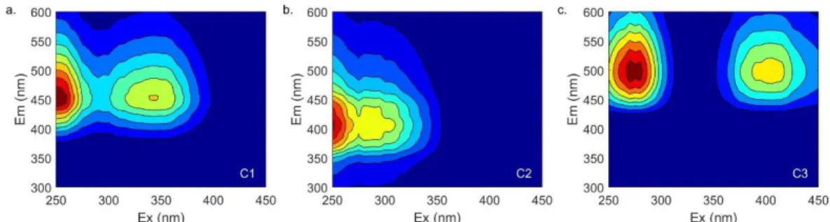
A three component PARAFAC model was fitted to collected FDOM samples (n = 472). Each component was split half, validated and matched with previously identified components on OpenFluor (Figure 2.3; Appendix 2, Table A2.2, Figure A2.2). FDOM Component 1 (FDOM C1) was identified as a terrestrial, humic-like component similar to Peaks A and C (Coble, 2007). FDOM Component 2 (FDOM C2) was identified as a microbial humic-like component, similar to Peak M, which has been linked to recent biological activity and is prevalent in eutrophic, human-impacted waters (Murphy et al., 2008). The component also contains
fluorescence in the peak A region, which is ubiquitous to aquatic environments. This component likely represents fluorescence from both of these regions (Peaks M and A), which are
co-occurring and following similar patterns in the estuary. Finally, FDOM Component 3 (FDOM C3) was identified as an additional indicator of terrestrial, humic-like material (Osburn et al., 2018). Results from the FDOM PARAFAC model indicate the FDOM pool is largely composed of humic-like material, mainly derived from terrestrial sources.
Table 2-2. OpenFluor matches for the 3-component FDOM model (TCC > 0.95). Matches were made on 01-14-2019. References are only a partial list of matches made on OpenFluor.
Ex max. (nm)
Em max. (nm)
OpenFluor Matches
Description Reference
C1 < 250, 345
454 19 Terrestrial,
humic-like, fulvic-acid like
Kulkarni et al., 2017; Osburn et al., 2018, 2016 C2 < 250 406 14 Terrestrial and
microbial, humic-like, estuarine, eutrophic waters, similar to M-peak
Cawley et al., 2012; Osburn et al., 2012; Yamashita et al., 2013
C3 270, 405 498 5 Terrestrial, humic-like Gueguen et al., 2014; Osburn et al., 2018; Yamashita et al., 2011 All three identified components (C1 – C3) had a statistically significant positive, linear relationship with DOC and DON (Appendix 2, Figure A2.4, Table A2.2). Therefore, like the dissolved fraction (DOC, DON), the three FDOM components decreased down estuary and with increasing salinity generally following conservative mixing (Figure 2.4; Appendix 2, Figure A2.5, Table A2.3), indicating all three components are of terrestrial origin. There were seasonal variations in the relationship between the various components (FDOM C1-C3) and salinity (Appendix 2, Figure A2.5, Table A2.3) which may reflect seasonally varying sources of terrestrial-like material from the riverine end member.
2015 study period, there were two identified storm events in the NRE (Hounshell et al., 2019) that could have resulted in the mobilization of watershed DOM from forested catchments leading to the increased fluorescence intensities observed in the estuary.
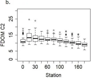
Figure 2-4. Boxplots of each of the three identified FDOM PARAFAC components plotted by station for all time points and depths.
inversely related to salinity, indicating these components were more prevalent at low salinities (i.e., in riverine water). The three FDOM components were also aligned with other fluorescence-derived measurements (Peaks B, T, N, M, A, C, HIX) which are often classified as indicators of terrestrial, humic-like material (Coble, 2007; Huguet et al., 2009). The three FDOM components were plotted opposite of BIX, which is a fluorescence indicator often linked with recent,
biological production of FDOM (Huguet et al., 2009). FDOM components were also distributed along PC2 with FDOM C1 and C3 clustered towards zero while FDOM C2 had positive PC2 loadings. FDOM C2 was clustered with fluorescence peaks that are typically indicators of material that are considered more biologically reactive (Coble, 2007), while FDOM C1 and C3 were clustered with fluorescence peaks identified as FDOM that is largely considered
recalcitrant. While the components (FDOM C1-C3) were identified as terrestrial in origin, PCA results indicate there were some potential differences in the lability of the FDOM material as identified in the FDOM PARAFAC model.
4.3BEFPOM PARAFAC modeling
A 5-component PARAFAC model was fitted to BEFPOM samples collected from the NRE (n = 476) (Figure 2.6, Table 2.3). Each component was split half validated and the first four
components (C1 – C4) matched with several previously identified fluorophores on OpenFluor (Table 2.3; Appendix 2, Figure A2.6). Most of the components matched (C1-C4) with
components previously identified in PARAFAC models that included BEFPOM samples (Brym et al., 2014; Osburn et al., 2015, 2012). BEFPOM component 1 (FPOM C1) was identified as a protein-like fluorophore most similar to tryptophan (Osburn et al., 2016). BEFPOM component 2 (BEFPOM C2) matched with components that have only been identified in models that include BEFPOM EEMs and are characteristic of eutrophic estuaries and microbial re-processing of FOM (Brym et al., 2014; Osburn et al., 2015, 2012). This component is essential in the
characteristic BEFPOM ‘three-peak pattern’ (Brym et al., 2014). BEFPOM component 3 (FPOM C3) was classified as a terrestrial, humic-like fluorescence peak that is indicative of fulvic acid-like fluorescence often derived from soil leachates (Graeber et al., 2012; Osburn et al., 2016). BEFPOM component 4 (FPOM C4) was identified as microbial, humic-like fluorescence similar to the previously identified Peak M and has been linked with recent biological production
Figure 2-6. 5-component PARAFAC model developed on collected BEFPOM samples. Table 2-3. OpenFluor matches for the 5-component BEFPOM model (TCC > 0.95). Matches were made on 01-14-2019. References are only a partial list of matches made on OpenFluor.
Ex max. (nm)
Em max. (nm)
OpenFluor Matches
Description Reference
C1 280 336 21 Protein,
tryptophan-like
Brym et al., 2014;
Osburn et al., 2016, 2012
C2 255, 360 456 3 FPOM specific,
eutrophic estuaries, microbial reprocessing of terrestrial DOM
Brym et al., 2014;
Osburn et al., 2015, 2012
C3 260 516 33 Terrestrial,
humic-like, fulvic-acid humic-like, soil leachates
Brym et al., 2014; Osburn et al., 2012; Shutova et al., 2014 C4 <250,
310
438 44 Marine and terrestrial humic-like,
combination of A and M peaks, possibly photo-labile
Brym et al., 2014; Murphy et al., 2008; Yamashita et al., 2013
C5 265, 345 448 1 Similar to humic peak C, terrestrial-like; un-characterized
Søndergaard et al., 2003
autochthonous components produced in situ as well as terrestrial like-components that are diluted, or potentially removed down estuary (Figure 2.7). Like the FDOM components, FPOM components that were characterized as terrestrial, humic-like decreased down estuary and
followed a typical conservative mixing pattern (Markager et al., 2011) (Appendix 2, Figure A2.8, Table A2.5). For the FPOM results, these terrestrial components included C3 which was
identified as a terrestrial, humic-like component with similarities to soil leachate and C4 which was classified as a marine/terrestrial humic-like component. The three components (FPOM C1, C2, C5), which increased in intensity down estuary, were most likely produced within the estuary (i.e., microbial or phytoplankton production) (Markager et al., 2011). These components include C1 which was characterized as protein, tryptophan-like, C2 which was characterized as FPOM specific and was indicative of microbial reprocessing of terrestrial DOM, and C5 which was un-characterized. I hypothesized that the previously un-characterized C5 component was likely a biological byproduct that was produced in the estuary and may be unique to BEFPOM samples.
Figure 2-8. PCA results for FPOM parameters. a. Sample scores plotted by season. b. Variable loadings plotted in PCA space. Variables are identified on the plot.
PCA was also applied to FPOM modeling results and associated POM variables (Figure 2.8). The 5 identified BEFPOM components were distributed along principal components axis 2 (PC2), such that components identified as terrestrial, humic-like material had negative PC2 loadings and were clustered with other indicators of terrestrial, humic-like material (SUVA, Peak C). Components characterized as more marine and biologically produced had positive PC2 loadings and were clustered with indicators of more recent, biologically produced OM (BIX). Unlike the FDOM pool which was almost entirely dominated by terrestrial, humic-like FOM, the FPOM pool included FOM sources from both terrestrial and autochthonous sources.
4.4FDOM+BEFPOM PARAFAC modeling
identified for the combined (FDOM+BEFPOM) model were almost identical to the components identified for the BEFPOM model. Components included a humic-like, microbial peak
(FDOM+BEFPOM C1); a terrestrial, humic-like peak (FDOM+BEFPOM C2); a FPOM specific component (FDOM+BEFPOM C3); a protein-like tryptophan component (FDOM+BEFPOM C4); and an un-characterized component (FDOM+BEFPOM C5) linked to biological production in the BEFPOM model developed for the BEFPOM samples only.
Table 2-4. OpenFluor matches for the 5-component FDOM+BEFPOM model (TCC > 0.95). Matches were made on 01-22-2019. References are only a partial list of matches made on OpenFluor. Ex max. (nm) Em max. (nm) OpenFluor Matches
Description Reference
C1 <250, 310
412 43 Terrestrial,
humic-like, similar to marine humic-like M peak
Brym et al., 2014; Murphy et al., 2008; Osburn et al., 2012
C2 260 506 38 Terrestrial,
humic-like, fulvic acid-humic-like, soil leachate
Brym et al., 2014; Murphy et al., 2014; Osburn et al., 2016
C3 255, 360 456 3 FPOM specific,
microbial re-processing of terrestrial DOM, nutrient impacted estuaries
Brym et al., 2014;
Osburn et al., 2015, 2012
C4 280 336 21 Protein-like,
tryptophan
Brym et al., 2014; Cawley et al., 2012; Osburn et al., 2012 C5 275, 345 448 1 Similar to humic peak
C, terrestrial-like, un-characterized
Søndergaard et al., 2003
When plotted against salinity and by station, the identified FDOM+BEFPOM components as applied to either FDOM or BEFPOM samples showed similar patterns as components identified for the individual FDOM and BEFPOM models (Appendix 2, Figure A2.11, Table A2.7;
production and degradation, more so than mixing processes between the riverine and marine end-members alone (Markager et al., 2011). Additionally, the fluorescent intensity of protein-like components, including tryptophan are often higher in the marine compared to the riverine end member, due to biological production in marine systems (Stedmon and Markager, 2005). Therefore, I expect the source of this component was both production in the estuary (as
phytoplankton and microbial production) and mixing with the marine end member (i.e., Pamlico Sound).
For the BEFPOM samples, the patterns were essentially the same for the combined model (FDOM+BEFPOM) and the individual model (BEFPOM), where terrestrial-like components (FDOM+BEFPOM C1, C2) decreased down estuary and biologically reactive components increased down estuary (FDOM+BEFPOM C3, C4, C5) (Appendix 2 Figure A2.14, Table A2.9). Results from the combined model (FDOM+BEFPOM) as applied to the FDOM and BEFPOM samples further highlight the dichotomy between the two pools: the FDOM pool was dominated by terrestrial FDOM while the BEFPOM pool was a combination of terrestrial FOM sources from the watershed (i.e., terrestrial sources) and biological sources (i.e., phytoplankton biomass) produced in the estuary.
samples. The C4 component was identified as protein-like, specifically tryptophan, and has been identified as a biologically-produced component in the FDOM pool (Coble, 2007).
4.5PARAFAC model comparisons
Results from TCC comparisons between PARAFAC models (FDOM, BEFPOM,
Table 2-5. Model comparisons between the three PARAFAC models generated for samples collected from the NRE: the 3-component FDOM model, component BEFPOM model, and 5-component FDOM+BEFPOM model. An X indicates 5-components which were > 95% similar.
FDOM C1 FDOM C2 FDOM C3 BEFPOM C1 BEFPOM C2 BEFPOM C3 BEFPOM C4 BEFPOM C5 BEFPOM C1 BEFPOM C2 BEFPOM C3
BEFPOM C4 X
BEFPOM C5 FDOM+BEFPOM
C1
X X
FDOM+BEFPOM C2 X FDOM+BEFPOM C3 X FDOM+BEFPOM C4 X FDOM+BEFPOM C5 X
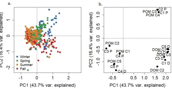
All the identified components from the three models (FDOM, BEFPOM, FDOM+BEFPOM applied to FDOM samples, FDOM+BEFPOM applied to BEFPOM samples) were plotted in PCA space (Figure 2.10). Because the BEFPOM model and FDOM+BEFPOM model applied to BEFPOM samples were exactly the same, each of the coupled components from these two models were clustered together in PCA space. Similarly, all FDOM components and
FDOM+BEFPOM components applied to FDOM samples were clustered together along the positive loadings of principal component axis 1 (PC1), except for C4d which was more closely associated with the three biologically produced BEFPOM components. C4d was the only
component identified as being a biologically produced DOM fluorophore, while all other FDOM components were identified as terrestrial, humic-like components. The two BEFPOM
Figure 2-10. PCA results as applied to components from all three models (FDOM, BEFPOM, FDOM+BEFPOM applied to FDOM samples, FDOM+BEFPOM applied to FPOM samples). a. Sample scores plotted by season. b. Variable loadings plotted in PCA space. DOM C1-C3
indicate components identified in the FDOM model. POM C1-C5 indicate components identified in the BEFPOM model. C1-C5 P and C1-C5 D indicate BEFPOM and FDOM components identified in the combined FDOM+BEFPOM model, respectively.
Results from the three models (FDOM, FPOM, FDOM+BEFPOM) and from the model comparisons, suggest the FDOM pool is largely composed of terrestrial, humic-like material while the BEFPOM pool contains fluorophores identified as both terrestrial-like and as autochthonous components produced within the estuary. Model comparisons suggest the
combined model (FDOM+BEFPOM) was almost entirely dominated by fluorescence variability in the BEFPOM pool.
4.6FluorMod estuarine signal
Figure 2-11. Plots of Chl a through time for each of the experimental bioassays used to identify an FDOM estuarine processing signal. Results were plotted by bioassay.