5276.pdf

(1)

Development of a Carbon Nanotube-Based Micro-CT and its Applications in

Preclinical Research

Laurel May Burk

A dissertation submitted to the faculty of the University of North Carolina at Chapel Hill in partial fulfillment of the requirements for the degree of Doctor of Philosophy in the

Department of Physics and Astronomy.

Chapel Hill 2013

Approved By

Dr. Otto Zhou (advisor)

Dr. J. Larry Klein, M.D.

Dr. Yueh Z. Lee, M.D.

Dr. Jianping Lu

(2)

(3)

iii

ABSTRACT

LAUREL MAY BURK: Development of a Carbon Nanotube-Based Micro-CT and its Applications in Preclinical Research

(Under the direction of Dr. Otto Z. Zhou)

Due to the dependence of researchers on mouse models for the study of human disease, diagnostic tools available in the clinic must be modified for use on these much smaller subjects. In addition to high spatial resolution, cardiac and lung imaging of mice presents extreme temporal challenges, and physiological gating methods must be developed in order to image these organs without motion blur. Commercially available micro-CT imaging devices are equipped with conventional thermionic x-ray sources and have a limited temporal response and are not ideal for in vivo small animal studies.

Recent development of a field-emission x-ray source with carbon nanotube (CNT) cathode in our lab presented the opportunity to create a micro-CT device well-suited for in vivo lung and cardiac imaging of murine models for human disease. The goal of this thesis

work was to present such a device, to develop and refine protocols which allow high resolution in vivo imaging of free-breathing mice, and to demonstrate the use of this new imaging tool for the study many different disease models.

(4)

iv

respiratory- and cardiac-gated live animal imaging on normal, wild-type mice is achieved. In Chapter 4, respiratory-gated imaging of mouse disease models is demonstrated, limitations to the method are discussed, and a new contactless respiration sensor is presented which

(5)

v

ACKNOWLEDGEMENTS

First and foremost, I am deeply grateful to my advisor, Otto Zhou, for his guidance in this research and for facilitating a culture of collaboration and friendship within our lab which began before my tenure as a research assistant and will no doubt continue long past my graduation. I would also like to thank each member of our research group, past and present, including Christy Inscoe, Mike Hadsell, Andrew Tucker, Emily Gidcumb, Lei Zhang, Jing Shan, Pavel Chtcheprov, Marci Potuzco, Jabari Calliste, Guohua Cao, Jerry Zhang, Xin Qian, Shabana Sultana, Xiomara Calderon-Colon, David Bordelon, Ramya Rajaram, Sigen Wang, Tuyen Phan, Ko-Han Wang, and Matt Wait. Particular thanks goes to Yueh Lee for his guidance, and for teaching through example the importance of

inter-departmental collaborations.

I thank my collaborators in the UNC School of Medicine who provided me with animal models for the many studies which comprised my dissertation work, as well as the staff of the Biomedical Research Imaging Center and the Lineberger Cancer Center. These include Sha Chang, Hong Yuan, Jon Frank, Kevin Guley, Jon Volmer, Brian Button, Alessandra Livraghi-Butrico, Mauricio Rojas, Eunice Kang, Monte Willis, William Kim, Hirofumi Tomita, Nobuye Maeda, Sean McLean, Arjun Deb, Ryan Miller, and far too many others to list here by name.

(6)

vi

(7)

vii

gating from each respiration sensor. Two separate lines were traced from each of the left and right lungs to the diaphragm (four lines total per CT image) to obtain average slope values. [8] ... 106 Table 5-1. Average respiratory and cardiac rates for subjects at each time-point. ... 129 Table 5-2: Infarcted volumes calculated as a percentage of the total

left ventricle wall volume, derived from computed tomography images and from TTC-stained histological slices. ... 143 Table 6-1(a): Quantitative comparison of restriction criteria ... 157 Table 6-1(b): Quantitative comparison of number of removed projections ... 157 Table 6-2: Average x-ray energy for various anode voltages and filter

materials, derived from simulations. The typical settings used for Charybdis, in italics, most closely match the k-edge of iodine,

(13)

xiii

LIST OF FIGURES

Figure 1-1: The first radiograph image taken by Roentgen, of his wife’s hand [2]. ... 2

Figure 1-2: Coherent scattering of an x-ray photon by an atom. [3] ... 3

Figure 1-3: The photoelectric effect. [5] ... 5

Figure 1-4: Compton scattering of an x-ray by an atom. [3] ... 6

Figure 1-5: the contributions by different physical interactions to the mass attenuation coefficient of soft tissue over a range of energies. [4] ... 8

Figure 1-6: Diagram of a conventional x-ray tube with stationary anode and heated filament cathode. [4] ... 9

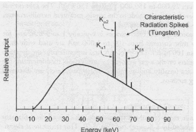
Figure 1-7: Energy spectrum of x-rays generated by a 90 kVp tube with an anode target. The broad energy curve of Bremsstrah- lung is dominant, with sharp energy spikes corresponding to the Kα and Kβ energies for tungsten. [4] ... 11

Figure 1-8: The effects of different focal spot size (filament size in traditional x-ray sources) and anode angle. [4] ... 12

Figure 1-9: Physical depiction of the theory behind algebraic-based CT reconstruction. Each linear attenuation path can be decomposed into the contributing voxel components and those components can be solved for directly. [5] ... 17

Figure 1-10: Attenuation ranges in HU for various relevant materials. [5] ... 18

Figure 1-11: The effect of geometry on image magnification. [3] ... 20

Figure 1-12: Example of line spread functions for two different kinds of film with different spatial resolutions. [3] ... 21

Figure 1-13: Sample MTF curves corresponding to the line spread functions shown in Figure 1-12. [3] ... 21

Figure 1-14: common CT image artifacts including (a) patient motion, (b) beam hardening, (c) partial volume, (d) metal implant (beam hardening), and (e) exceeding field of view ... 22

(14)

xiv

Figure 2-2: (a) A schematic of the triode-type field emission x-ray tube with SWNT cathode. The gate electrode is a metal mesh 50–200 mm away from the cathode. Electron emission is triggered by the voltage applied between the gate and the cathode. X-ray is produced when the emitted electrons were accelerated and bombarded on the copper target. (b) The emission current transmission rate Ia / (Ia1Ig) versus anode

voltage (Va) measured in the triode configuration at different gate voltages. (c) Energy spectrum of the x ray generated from a copper target at an acceleration voltage of 14 kV. [10] ... 37 Figure 2-3: X-ray projection images acquired using an early CNT

x-ray source and Polaroid™ films. Imaging subjects included (a) a fish and (b) a human hand. X-ray parameters were 14 kVp and 180 mAs. X-ray output and applied gate voltage are plotted over time (c) when operated at 1 kHz and 50% duty

cycle. The height of the signal indicates the photon energy rather than the intensity. [10] ... 37

Figure 2-4: The procedure used to create a CNT cathode through EPD. On inset figures, optical microscope images of a cathode after (a) photolithography, (b) CNT deposition, and (c) liftoff with NMP and vacuum annealing. [14] ... 39 Figure 2-5: SEM images showing the top surface of the composite

CNT film both: (a) before and (b) after vacuum annealing. The CNTs are randomly oriented on the surface. (c) Cross-sectional SEM image of the CNT cathode after the activation process. The surface CNTs are now vertically aligned in direction per- pendicular to the substrate surface. Cross-sectional SEM images of two cathodes fabricated under the same conditions except different CNT concentrations in the EPD inks. Cathode

shown in (e) was made using an ink with 4× the CNT concentration than the cathode shown in (d). [14] ... 40 Figure 2-6: (a) Field emission current as a function of the applied

gate voltage from a 0.50 mm × 2.35 mm elliptical CNT cathode at constant anode voltage. For comparison the data from the same cathode measured in the parallel-plate geometry (cathode –to –anode spacing was 150 μm) is also shown. (b) Emission lifetime measurement of a 0.50 mm × 2.35 mm CNT cathode at constant current mode in triode geometry. [14] ... 42 Figure 2-7: (left) Schematics of CNT configuration on the surface.

(15)

xv

direction. (middle) SEM pictures of CNT film. (right) The 3 distribution model studied (a) No beam divergence assumed where all the particles are emitted at an angle of 90° from the emission surface. (b)The random distribution model, and (c) The forward biased model. [15] ... 43 Figure 2-8: Plot of the FSS (axis) as a function of the top focusing

voltage for a 2.35 x 0.5 mm cathode, operating at 40KV anode voltage and about 1300V gate voltage for 0.2mA cathode current. The simulated results for the 3 different beam dist- ributions have been compared with actual experimental data. The experimental measurements show best agreement with the forward biased beam distribution in terms of both FSS size and also transmission rate. This confirmed the accuracy of the emission model and from here on the forward biased distribution has been used for all the electron optics simulations. [15] ... 44 Figure 2-9: (left) Shows the beam divergence after passing through

the 2D gate mesh which is used for extraction of the electron from the emission surface. The particles cross-over dramatically making it very difficult to focus them back to a point on the anode surface. (right) When the gate mesh is replaced by a 1D linear mesh, the particles display less divergence making it easier to focus the beam to a small focus spot. [15] ... 45 Figure 2-10: (left) are the optical images of the 2D mesh and 1D

mesh. (right) The measured FSS as a function of the top focusing voltage at 40KV anode voltage and 1200V gate voltage. An isotropic 100μm FSS is obtained using the 1D mesh which is smaller than the FSS using the 2D mesh. [15]... 45 Figure 2-11: (left) Representative current density distribution

(simulated) on the anode surface. A Gaussian fitting is done to obtain the FSS, which is defined as the area within which 80% of the anode current resides. (right) Comparison of the transmission rate between simulation and experimental. There is an overall gain in anode transmission using the 1D mesh. [15] ... 46 Figure 3-1: The prototype CNT-based micro-CT scanner and

(16)

xvi

Figure 3-2: Representative samples of the respiration signals from the BioVet physiological monitoring system with the corresponding physiological triggers (red dotted squares) superimposed at the corresponding phase portions of the respiration cycles. These physiological triggers are gated with the exposure windows to generate the x-ray triggers, as illustrated in figure 2(b). X-ray imaging windows were 50 ms in duration for both peak inspiration (a) and end expiration (b). [1] ... 51 Figure 3-3: (a) Diagram of workflow in the CNT micro-CT system.

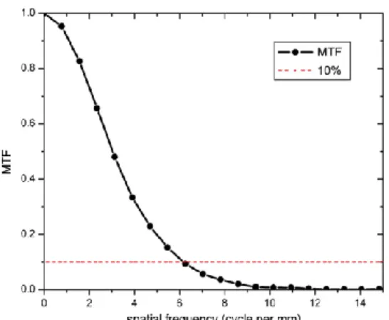
The scanner is controlled by a computer running an automated control program written in LABVIEW. Subject physiology is monitored simultaneously with the camera frame rate and x-ray source readiness. If the simultaneity gating condition is satisfied, and only when this condition is satisfied, an x-ray pulse is triggered by the controlling computer. (b) A diagram of the timing for physiologically-gated image acquisition. When the subject’s desired abdominal position coincides with the fixed frame rate of the detector, an x-ray projection is acquired, followed object rotation. [1] ... 51 Figure 3-4: Configuration for the system temporal resolution measurement. [1] ... 54 Figure 3-5: System MTF measurement for the prototype CNT micro-CT. ... 56 Figure 3-6. Reconstructed CT image slice of the contrast phantom

comprised of (1) air, (2) water, (3) fat mimic, (4) iodinated contrast agent and (5) bone simulating material. [1] ... 56 Figure 3-7: Temporal response of the dynamic micro-CT scanner.

Images were taken at 40 kV, 0.7 mA anode current and various x-ray pulse widths. For the reference purpose, shown in the very right is an image taken from single 100 ms x-ray pulse exposure when the wire was static, followed by the images of the moving wire taken at 100 ms, 50 ms, 20 ms, 10 ms and 5 ms pulse width. [1] ... 57 Figure 3-8: Axial (a) and coronal (b) reconstructed slices from a

(17)

xvii

Figure 3-9: Axial and coronal slices from an in vivo CT of the same mouse. Images were reconstructed from two consecutive scans of a single mouse using the same imaging protocol at 62 × 62 × 62μm3 isotropic voxel size. Images shown are from peak inspiration (a) and (c), and full exhalation (b) and (d) in the axial and coronal views, respectively. [1] ... 59 Figure 3-10: Pictures of (a) the CNT-cathode field emission micro-

focus x-ray tube and (b) the tabletop micro-CT scanner, com- posed of the CNT x-ray tube, a CsI flat-panel detector, a small- bore goniometer, and a horizontally-oriented stationary mouse bed. The x-ray tube’s body dimension is 150 mm x 70 mm x 70 mm. The CT scanner is operated in a step-and-shoot mode; a full scan is completed in one rotation of the cone-beam x-ray source. [6] ... 63 Figure 3-11: A CAD rendering of the CNT micro-CT imaging

system offers a slightly less cluttered view of the system. The rotating gantry, x-ray source, detector, and mouse bed are labelled... 64 Figure 3-12: A representative respiratory trace from a single animal,

with x-ray pulses (actual temporal width) superimposed at peak inspiration (a) and end-expiration (b). X-ray pulses are fired only during breaths where the respiration phase of interest synchronizes with the x-ray exposure window. [7] ... 66 Figure 3-13: Axial (top) images through the lower lung of a single

animal and reformatted coronal (bottom) images obtained at the same slice location obtained during the peak inspiration (a, c) and full expiration (b, d) portions of the respiratory cycle. [7] ... 68 Figure 3-14: Shaded surface renderings of a mouse lung and trachea

in inspiration (a) and expiration (b). Differences in the shape and

volume of the lungs in each respiratory phase are easily distinguished. [7] ... 69 Figure 3-15: (a) Illustrative timing diagram for the dynamic gating

(18)

xviii

Figure 3-16: (a) and (b) Axial and (c) and (d) coronal slice images of a C57BL/6 mouse at (a) and (c) 0 and (b) and (d) 55 ms after the R wave. All images have the same display window and level. The voxel spacing in- and out-of-plane is 76 microns. Major anatomic structures of the cardiopulmonary vascular system are readily identified in the contrast enhanced images. The aorta (AO), left ventricle (LV), and right ventricle (RV) are labeled for reference. [6] ... 73 Figure 3-17: Intensity profiles along the two lines within the

images shown in Figure 3-16a and b. For each intensity profile, the two boundary regions between the ventricles and the ventricle wall were linearly fit. The derived slopes are shown in Table 3-4. The three (IVS, VW, and LV) sections of the line profiles are labeled in the plot. The width at the midheight of the IVS section changed from 1.3 mm at 0 ms to 1.8 mm at 55 ms, representing a change of 0.5 mm in the ventricle wall thickness from diastole to systole. [6] ... 74 Figure 4-1: Axial lung slices of respiratory-gated micro-CT imag-

ing of two female Kras+/Luc+ mice imaged at 3-week intervals. Compared with the earlier time point (left), later images (right) show both a greater number of lung tumors and a growth in diameter of individual tumors. ... 80 Figure 4-2: 2D optical imaging of four female mice: two control

subjects (left) and two Kras+/Luc+ mice (right), twenty weeks after initial inoculation with tumor cells. At bottom, corresponding axial CT slices of each of the four mice are displayed at a matching timepoint. The total luciferase optical signal increase compares with an increase in total tumor load, although detailed structure of the lungs and any present tumors is not visible. ... 81 Figure 4-3: (a) 3-D rendering of the lungs of a mouse exhibiting

tumors during the first imaging timepoint. (b) Axial, (c), sagittal, and (d) coronal views of the CT volume during the region growing algorithm in ITK-Snap. ... 82 Figure 4-4 (left): Estimated tumor volume measurement (sum of

(19)

xix

Figure 4-5: Semi-transparent 3-D rendering of healthy (left) and tumor burdened (right) mouse lungs. Images were generated using OsiriX processing software and in vivo respiratory- gated micro-CT images ... 83 Figure 4-6: Axial (top) and Coronal (bottom) CT slices acquired at

three-week intervals of a control animal (time elapsing left to right). ... 86 Figure 4-7: Axial (top) and Coronal (bottom) CT slices acquired at

three-week intervals of a mouse exhibiting multifocal lung tumors (time elapsing left to right). ... 86 Figure 4-8: Contrast-enhanced images of the lung and other nearby

organs. With the hepatic agent on board, the liver is now able to be distinguished from the gallbladder, and the spleen is brightly illuminated ... 89 Figure 4-9: Effect of atelectasis on in vivo lung imaging. Partial

lung collapse of the left lung of an adult mouse is seen in reconstructed axial (A) and sagittal (B) CT slices; 3-D volume renderings of the airspaces display the effect of atelectasis more dramatically in front (C) and rear (D) views. ... 90 Figure 4-10: The plastic mouse bed allows the animal to lie prone

with its head inside the nose cone for gaseous anesthesia deliv- ery, and the non-contact displacement sensor is positioned a few millimeters away from the animal’s ribs. The design allows simultaneous testing of the pressure and non-contact sensors with murine subjects. [7] ... 93 Figure 4-11: A schematic of the timing structure employed in pro-

spective gating is shown above. X-rays are to be fired only during the maximum inhalation phase of respiration, but this must also fall within the acquisition window of the fixed-frame rate flat panel detector. When these two conditions are met, the x-ray is switched on to acquire a projection image, and the gantry is then rotated to await the next synchronized event. [8] ... 95 Figure 4-12: The custom-built CNT cone beam micro-CT used in

(20)

xx

Figure 4-13 Left. Simultaneously-acquired respiration traces from the standard pressure sensor (top) with x 20 signal amplification and the non-contact displacement sensor (bottom) with x2 amplification are displayed in the BioVet GUI. Right. For seven CT scans, the signal traces from both respiration sensors are analyzed to define the timepoint of maximum sensor output (ms) for each breath. [8] ... 102 Figure 4-14. Comparison curves showing the relationship between

the signals from the noncontact and pressure-based sensors. The four plots demonstrate this relationship during scans of the four subjects. Each data point on the curves corresponds to one 2 ms time period in the 300 ms-defined breath cycle. Parti- cularly noticeable are the asymmetry of the upper and lower branches of the curves and their generally non-linear shape despite the temporal matching of the breath peak and trough. [8] ... 103 Figure 4-15. Transverse, coronal, and sagittal CT slices of an adult

wild-type using the non-contact (a) and pressure (b) sensors to monitor and prospectively gate to respiratory motion. During the acquisition of each image, both the fiber-optic cable from the displacement sensor and the plastic tubing from the pneu- matic sensor were included in the field of view so that image artifacts arising from these structures would be comparable between the two scans. [8] ... 105 Figure 4-16: Line plots were measured across the lung/diaphragm

boundary at four different locations in the left and right lungs (two line plots per lung) for each image acquired. The slope of the path across the boundary was measured for each gating protocol (pressure or noncontact sensor) and compared for each of the four subjects. [8] ... 106 Figure 4-17: Respiration-gated micro-CT of the knockout hernia

model. In the mid-lung axial slice (a), note that the liver app- ears to have displaced one lung (animal’s right, image left). In what should be the mid-liver slice (b), the bowels and lower

organs have been displaced upwards in the body and are in contact with the lower parenchyma of the lungs. [8] ... 107 Figure 4-18: (a) Reconstructed axial slices of respiratory - gated

(21)

xxi

Figure 4-19: A prospectively-gated CT image of a 9-day-old mouse pup using the pressure-based sensor to monitor and gate to respiration motion. The pressure required for use of this sensor results in high rates of atelectasis in the left lung (seen here as a complete pneumothorax). [8] ... 109 Figure 4-20: CT transverse and coronal slices of 11-day-old mouse pups imaged without respiration gating (a), (c), and using prospective respiration gating from the laser-displacement non- contact sensor (b), (d).. Fine details of the lungs are more clearly visualized with respiration gating, as is the definition between lungs and diaphragm (indicated with arrows). [8] ... 110 Figure 5-1: Micro-CT of aortic calcification using CNT micro-CT

(left) and a commercial micro-CT system (right). CNT micro- CT images display lower noise and sharper edge definition [7]. ... 119 Figure 5-2: A, Representative carbon nanotube micro-CT images

of 129-apoE KO and B6-apoE KO mice. White areas at the inner curvature of the aortic arch indicate calcifications. B, Cal- cification volume in the aortic arch of the 2 strains. C, Represen- tative images of excised aortas. D, Comparison between the 2 strains of plaque areas in the aortic arch. E, Representative arch plaques by cross-section stained with Sudan IV and counter- stained with hematoxylin. Arch calcification was detected by von Kossa staining (brown, arrows). Scale bar, 200 lm. CT indicates computed tomography; KO, knockout [7]. ... 121 Figure 5-3: Myocardium wall thicknesses during systole, measured

from micro-CT images, increase along with the time elapsed since the TAC procedure. Similarly-proportioned enlargement is seen in both the interventricular septum and the inferior wall of the left ventricle; the growth of each is approximately 10- 12% over the study’s four week period. ... 126 Figure 5-4: (a) Axial and (b) coronal CT views of control subjects.

(22)

xxii

Figure 5-5: Ejection fraction for subjects at the control time-point and at 2-weeks and 4-weeks post-banding. Although EF decreases as expected soon after banding, partial recovery of function is seen by the 4-week time-point. ... 129 Figure 5-6. A flow-chart visualization of the contrast administra-

tion and imaging protocol of this work. Four micro-CT images were acquired using two iodinated contrast agents, Iohexol

300 mg I/mL and Fenestra VC. Images were acquired during either diastole (on r-wave) or systole (55 ms delay from r- wave). The acquisition of each gated micro-CT image required 10 to 15 minutes. After successful completion each stage of the protocol, the next immediately commenced. ... 137 Figure 5-7. Micro-CT images of the ischemia reperfusion murine

model. Images taken an average of 13 (a) and 30 (b) min after administration of Iohexol show obvious delayed contrast enhancement of infarcted tissue. ... 140 Figure 5-8. CT numbers (in Hounsfield units) were measured for

regions-of-interest comprised of the blood pool, myocardium, and infarct regions for each of the first two acquired CT images of each subject. Delayed hyperenhancement occurs in both visualized timepoints following the administration of Iohexol but is strongest during the first image acquisition ( an average of thirteen minutes after injection). While the CT numbers for blood and infarct are similar in many of the images, the two are easily distinguishable within the context due to the location of the infarct, which is always imbedded within the myocardial wall. Both blood and infarct are clearly distinguishable from myocardium in all Iohexol-enhanced images. This is particularly true during the first of the two observed time points. ... 141 Figure 5-9. Areas of delayed iodine contrast enhancement in the

infarcted myocardium are visible in micro-CT images (upper left) due to contrast agent retention in fibrotic tissue. These portions of infarcted myocardial tissue appear on histological slices stained with TTC ( Triphenyl tetrazolium chloride) in pale pink due to their lack of marker uptake (upper right). Indi- cators for infarcted myocardium are comparable in location, shape, and volume in both CT grayscale images and stained histological slices. ... 142 Figure 6-1: A typical “average breath” signal (mean over 400 breath

(23)

xxiii

Figure 6-2: (a) A coronal CT slice indicating the path of the five- pixel-wide slope measurement across the diaphragm and right lung. (b) The gradient is calculated along the path for the original unrestricted image set and all six of the restricted image

sets. ... 156 Figure 6-3 : Comparisons between diaphragm slopes of original un-

corrected image sets and those of image sets with five percent of projections removed as determined by: the correlation coefficient (upper left), mean breath height (upper right), mode breath height (lower left), and all combined criteria (lower right). ... 157 Figure 6-4: Comparisons between diaphragm slopes of original un-

corrected image sets and those of image sets with (a) 10, (b) 20, (c) 40, and (d) 80 of the original 400 total projections removed after being selected due to low correlation coefficients. The ratio of new slope to uncorrected slope is displayed on the vert- ical axis; data points located above the y=1 line represent im- provement in image quality as quantified by the chosen metric. ... 158 Figure 6-5: (a) An axial CT slice of the heart and lungs, with resp-

iration gating and no additional corrections is displayed. (b) The same axial slice is shown after five percent of the total 400 projections (those whose corresponding breaths have the lowest correlation coefficients compared with the mean breath shape) were removed prior to reconstruction. ... 160 Figure 6-6: Plots of breath width versus projection (breath count)

number for three different micro-CT scans corresponding to (a) flat, (b) stair-step, and (c) incline trends. ... 164 Figure 6-7: There is a characteristic, roughly-inverse relationship

over time between (a) the measured breath height and (b) the breath width for a single animal and micro-CT imaging session. These physical variables are dependent due to the subject’s minute oxygen needs which must be met regardless of respiration rate. ... 165 Figure 6-8: A characteristic stair-step change in breath height (a),

(24)

xxiv

Figure 6-9: Simulated energy spectrum from the Charybdis micro- focus tube, with tungsten target, 0.2 mm Be window and additional 0.5 mm Al filter. ... 170 Figure 6-10: Axial CT slices (left) and line profiles (right), before

bilateral filtration (top), and after filtration using a filter with width of 1 pixel (middle) and 5 pixels (bottom) ... 173 Figure 6-11: Axial (left), coronal (center), and sagittal (right) micro-

CT slices of an adult male mouse with a U87 brain tumor which grew from cells implanted three weeks prior to imaging. Cont- rast enhancement within the skull indicates tumor size and lo-

(25)

1. Background and Motivation

1.1 X-rays

1.1.1 Discovery of X-rays

On November 8th, 1895, Roentgen (50-year-old professor of Physics at Julius Maximilian University of Wurzburg, Germany), testing his cathode ray tube, saw a glimmer of light from his barium platinocyanide fluorescent screen, which was located over a meter away from the cathode ray tube. He had discovered “eine neue Art von Strahlen” – “a new kind of rays” [1]. Roentgen had been looking for the “invisible high-frequency rays” predicted by Hermann Ludwig Ferdinand von Helmholtz, which had been predicted based on from Maxwell’s theory of electromagnetic radiation. Roentgen called these rays X-strahlen – “x-rays”, x for unknown [1].

(26)

2

Figure 1-1: The first radiograph image taken by Roentgen, of his wife’s hand [2]. 1.1.2 Properties and Characteristics

X-rays are electromagnetic waves with wavelengths ranging from approximately 100 nm to 0.01 nm. Their propagation and properties are understood not only as waves governed by Maxwell’s Equations, but also as particles using the principles of quantum mechanics. In medical imaging it is often helpful to think of x-rays as discrete photons, each possessing energy related to the frequency ν and wavelength λ by

where h is Planck’s constant.

(27)

3

angiography, breast cancer screening (mammography and digital breast tomosynthesis), and computed tomography (CT).

1.1.3 Photon-Matter Interactions

The utility of x-rays for medical and other imaging devices is made possible because of the interaction between photons and matter, resulting in absorption or deflection of some number of photons from their direct path to a detector or film. The dominant interactions between photons and physical matter include coherent scattering, the photoelectric effect, Compton scattering, and pair production. A brief description of each follows.

Coherent Scattering

Coherent scattering is an elastic collision between the incoming photon and an atom within the target material. This scattering, which is a classical rather than quantum effect, most generally is seen in interactions between matter and low-energy radiation. Of all the interaction types we consider, it is the only one which is non-ionizing. Where coherent scattering is present in x-ray medical imaging, it does not contribute to patient dose but it does contribute heavily to image noise, deteriorating image quality.

Figure 1-2: Coherent scattering of an x-ray photon by an atom. [3]

(28)

4

(29)

5

photoelectron is left free to collide with atoms of nearby tissues causing DNA damage, none of this dose is wasted, and it is entirely necessary for image production.

Figure 1-3: The photoelectric effect. [5]

Compton Scattering

While a small amount of image-degrading scattered radiation comes from coherent scattering, the overwhelming majority is a result of Compton scattering. In this inelastic scattering interaction, only part of the x-ray photon’s energy is transmitted to the electron, while the rest is retained by the scattered photon. The amount of energy retained by the photon is a function of the ratio of the initial photon energy to the ejected

electron’s binding energy, and of the scattering angle. The well-known equation which describes the Compton Effect is

( ).

(30)

6

aforementioned generation of image-deteriorating noise, and a radiation safety hazard in the area surrounding the x-ray imaging procedure which must be contained with radiation shielding materials.

Figure 1-4: Compton scattering of an x-ray by an atom. [3]

Pair Production

The final matter-photon interaction, pair production, is only relevant for very high energies (~1 MeV), so it is of limited relevance for most medical x-ray imaging

applications. For photons of this very specific energy, interaction with the nucleus of the target material results in complete absorption of the photon and simultaneous production of an electron and positron pair (each of rest mass 511 keV). A somewhat related process, photodisintegration, occurs when a photon with energy equal to or greater than the

binding energy of nucleons dissipates its energy to nucleus, leading to the ejection of protons or neutrons from the target atom. As with pair production, this event is highly unlikely for a typical medical imaging application, and the loose-cannon behavior of free protons or neutrons in biological tissues would result in undesirable effects in a patient.

1.1.4 X-ray Attenuation and the Attenuation Coefficient

(31)

7

straight path through to the other side. Regardless of the method, whether by Compton scattering or the photoelectric effect or by a combination of other physics, the incoming beam will be attenuated in a statistical but ultimately predictable way, dependent upon the energy of the photons and various properties of the bulk material.

The simplest case to consider is a monoenergetic x-ray beam of initial intensity Io and a homogenous material into which the beam enters. The intensity of the x-ray beam will be attenuated exponentially as it travels through the homogenous material of thickness d. This will occur according to Beer’s law, which states that the outgoing

intensity is _{, where µ is a bulk property of the target material called the linear}

attenuation coefficient. If the initial x-ray intensity Io is known and the exiting intensity I can be measured directly, then assuming the path length d is also known, the numerical

value of µ can be solved forward straightforwardly as ( ). Because the

photon-matter interactions that are simplistically summarized by the single value µ are statistical, a sufficiently large number of photons must be included in Io in order to accurately

measure the linear attenuation coefficient; but assuming that this condition is met, µ is found trivially in the simple case.

Supposing that the target material is not homogenous but is instead made of several materials, each with their own linear attenuation coefficient, it is easy to conclude that the outgoing x-ray intensity I will be affected multiplicatively through each different

material with a path length dn and its linear coefficient µn, giving ∑ for the

intensity of an x-ray beam after a linear trajectory through the materials

(32)

8

truly a constant. Rather it depends upon the energy of the photons which interact with the material, so it is in fact best expressed as a function µ(E).

Figure 1-5: the contributions by different physical interactions to the mass attenuation coefficient of soft tissue over a range of energies. [4]

Additionally, µ depends upon a variety of physical properties such as density and atomic number. As a consequence, it is possible for two very different types of materials to have the same or similar linear attenuation coefficients. Thus while µ can be a helpful metric for comparing different materials, it is only meaningful in context and should be used cautiously.

For visual example, Figure 1-5 shows how a single material, soft tissue, exhibits different mass attenuation coefficients over a range of energies, and which mass-photon interactions contribute most to the attenuation coefficient at that energy.

1.1.5 X-Ray Tube Design

(33)

9

Figure 1-6: Diagram of a conventional x-ray tube with stationary anode and heated filament cathode. [4]

Cathode (electron source)

The source of electrons in a conventional x-ray tube is a helical filament cathode filament made of tungsten wire or a similar material. A voltage of up to 10 V is applied to this filament generating a current of 3 – 7 A, and electrical resistance produces heat so that electrons are released through thermionic emission [4]. Because the thermionic electron emission is not directional, a focusing cup which partially surrounds the cathode filament is held at a negative bias so that the resulting electric field bends the electron trajectory into a more focused beam.

Anode

The anode within the x-ray tube serves two important purposes. First, it is set at a high positive voltage with respect to the other tube components so that the electron beam is heavily accelerated towards it, gaining kinetic energy which will be imparted to the x-ray beam. Second, the material of the anode is appropriately chosen so that, when the electron beam bombards it, x-rays are generated. For this second purpose, the anode is also called the target material.

(34)

10

When accelerated electrons strike the anode material, the resulting x-rays are generated through two different mechanisms: these are Bremsstrahlung and characteristic radiation.

Bremsstrahlung

Sometimes known by the descriptive “white radiation,” Bremsstrahlung (German for “braking radiation”) is electromagnetic radiation emitted when one charged particle decelerates as it is deflected by another charged particle [4]. For the relevant scenario which occurs inside of an x-ray tube, the two charged particles of interest are accelerated electrons and the atoms of the anode target material. The energy of the photon emitted is equal to the kinetic energy lost by the charged particle during deceleration. The nickname of white radiation describes the broad and continuous distribution of this radiation across the energy spectrum, with the maximum cut-off energy equal to the initial kinetic energy of the electron as it enters the target material. This maximum energy can only occur, however, when the energy of the electron is converted into a single photon, which is a relatively rare event. Much more often, multiple photons are released per electron; as a result the energy spectrum of Bremsstrahlung (from many electrons with the same initial kinetic energy) is weighted more heavily to the lower end of the spectrum. The energy spectrum from a tube displays a drop-off at the lower energy end as well, but this can be attributed to filtration by the x-ray window material.

(35)

11

Characteristic x-rays are generated by an atom when outer-shell electrons collapse down into vacancies in the inner shells. The energy of the x-ray is equal to the difference between the energy levels of these two shells, and the photons are called “characteristic” because these energy level differences are particular to a given element. The

characteristic radiation energy levels for a given target material will appear in the x-ray spectrum as discrete peaks across the broad Bremsstrahlung energy spectrum (Figure 1-7).

Figure 1-7: Energy spectrum of x-rays generated by a 90 kVp tube with an anode target. The broad energy curve of Bremsstrahlung is dominant, with sharp energy spikes corresponding to the Kα and Kβ energies for tungsten. [4]

Anode design

(36)

12

Figure 1-8: The effects of different focal spot size (filament size in traditional x-ray sources) and anode angle. [4]

A large amount of heat is generated within the anode along with x-ray production, and this heat load can be a limiting factor in the amount of flux generated by an x-ray tube. The transmission of heat away from the anode is a major design concern. In

stationary anode configurations, it is common to insert the target material within a copper block which helps carry heat away. Most commercial x-ray sources feature a complex rotating anode rather than a simple stationary anode in order to spread the heat load over a much larger volume of material.

1.1.7 X-ray Tube Rating

The x-rays generated by a particular tube are characterized by (1) the cathode current, (2) anode voltage, (3) anode material, and (4) any additional filtration material. The cathode current and anode voltage together define the anode current of the tube, and thus the overall flux of x-rays emitted from the tube. The anode voltage and the anode material determine the energy spectrum of the photons generated through Bremsstrahlung and characteristic radiation. The spectrum and total number of photons are modified as the beam passes through any the filter material (including the x-ray exit window).

(37)

13

The fundamental design of the x-ray tube has changed very little since the developments made by William Coolidge many decades ago, with the exception of the rotating anode. Conventional x-ray tubes are the most commonly type of x-ray source, but they have some limitations. The thermionic filament cathode requires significant heating generation and high power consumption, contributing to a bulky system requiring external cooling. Also, the thermionic electron emission limits the temporal resolution of the system; electron emission cannot be switched rapidly with a filament cathode, and external mechanical shuttering must be used to create temporally narrow pulses. Finally, thermionic emission is spatially isotropic, requiring an additional focusing cup to direct the beam towards the anode, and the emitted electrons have a very wide energy

distribution.

1.2 Computed Tomography

1.2.1. Historical Background

(38)

14

This work was done independent of and unaware of Radon’s earlier publication, and it was only theoretical and he never applied it himself in imaging experiments.

G.N. Hounsfield is regarded as the true inventor of CT. Unaware of the earlier work by Radon and by Cormack, in 1972 he independently acquired and reconstructed the first computed tomography image of the head of a patient with a cystic frontal lobe tumor [5]. He did this with hardware manufactured by EMI Ltd, a company better known to most for their contributions in music as the recording company that signed the Beatles. The so-called “EMI scanner” maintained a total monopoly on the technology until

Siemens launched their own project in 1974. Hounsfield and Cormack were jointly awarded the Nobel Prize in medicine in 1979 for their contributions in the development of the CT scanner [5].

From rapid adoption of the new technology in the early eighties, very little progress was made until new scanning geometries such as spiral CT (developed by Kalender in 1989), and computing and detector technologies advanced to increase resolution and imaging speed. Since those new developments, the CTs have become an integral part of the clinic. In 2010, the number of CT operating in clinics is estimated to be above 50,000 [5]. Despite the availability of many other imaging modalities, the prominence of CT imaging is guaranteed for the near future.

1.2.2 System Components

(39)

15

translates) to facilitate acquisition from many angles. Generally, the patient lies on a stationary horizontal bed and the x-ray source is attached to a rotation gantry, but the exact geometric configuration of the CT components has been modified over time.

1.2.3 CT Generations – Technological Improvements

Although the basic physics of computed tomography and the general physical components of a CT scanner (x-ray source, detector, and rotation gantry) have not changed significantly over the years, scanning geometries have been modified over the years in a series of generations [4].

Pencil Beam

The original CT scanners featured a single pencil beam x-ray source which was both translated and rotated to provide full coverage of a sample slice. Two small detectors positioned opposite the pencil beam acquired images for two CT slices

simultaneously. This configuration resulted in very little scatter reaching the detector, but scan times were prohibitively long.

Narrow Fan Beam

The next generation followed the same translation and rotation path of the x-ray source, but the x-ray beam was now a narrow fan of approximately 10 degrees rather than a pencil, and the two-detector array was upgraded to a 30 detector linear array. Scan times decreased and scatter, while still minimal, increased.

Wide Fan Beam

(40)

16

patient. In the fourth generation, a stationary ring of detectors surrounds the patient and only the x-ray source rotates.

Helical geometry

With the development of slip-ring technology, the gantry is permitted to rotate continuously, increasing volume scan speeds. To take advantage of fast rotation speeds, a geometry was developed in which the patient bed is translated through the gantry linearly as the fan beam source rotates, effectively passing the beam in a spiral around the patient.

Cone beam CT

With a cone-beam x-ray source and a large 2-D detector positioned opposite, a full image acquisition can be acquired in a single gantry rotation. Due to the expense of building such a detector array, this configuration is only practical for imaging

applications with small fields of view, such as dental and head CT and micro-CT (see Section 1.3).The CNT micro-CT described in this work has a cone beam geometry.

A cone beam x-ray source must be capable of high flux in order to illuminate the entire imaging object at once within a short exposure time. Cone beam CT also has the drawback of allowing more scatter to reach the detector plane.

1.2.4 Theory of CT Reconstruction

In Section 1.1.4, it was seen that the total attenuation I/Io experienced by an x-ray

beam as it travels through a bulk of non-uniform material can be expressed by the sum

∑ _{or by the line integral} ∫ ( ) _. _[5]

(41)

17

rotation and pass through each volume segment many times in order to obtain sufficient information.

If a sufficient number and distribution of line integrals have been measured, an inverse transform can be performed to obtain all values of µ(x, y) within the object. The general principle behind an exact algebraic solution to this problem is visualized in Figure 1-9.

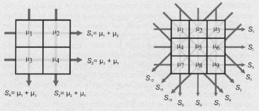
Figure 1-9: Physical depiction of the theory behind algebraic-based CT reconstruction. Each linear attenuation path can be decomposed into the contributing voxel components and those components can be solved for directly. [5]

This type of direct algebraic solution, however, is extremely time-consuming, so a method of convolution and back projection is generally performed instead. An exact solution could theoretically be obtained, but in practice there is a spatial sampling distribution which corresponds to frequency limitations in an image which has been inverted with a Fourier transform. To prevent the image distortion which results from sampling restrictions, different convolution kernels can be applied prior to the inversion / back projection algorithm, acting as a high pass filter to prevent the unsharpening of object edges which would otherwise occur in the final reconstructed volumes.

(42)

18

As described previously, the attenuation coefficient for a given voxel (3-D pixel or volume segment) derived by CT is not always physically meaningful because it

depends upon several variables including x-ray energy. In order to convert the attenuation coefficients to a meaningful range for diagnostic imaging, a scaling is applied to convert into Hounsfield units (HU). This weighting anchors values for water and air at 0 HU and -1000 HU, respectively, so that the CT values for any arbitrary tissue with attenuation

coefficient µT is given by ( )

. [5]

On this scale, HU for a given material can still have a range of values depending upon scanning parameters, but the values are anchored enough to give narrow ranges within the typical settings for clinical CT. Figure 1-10 shows common attenuation ranges in HU for various materials within the human body.

Figure 1-10: Attenuation ranges in HU for various relevant materials. [5] 1.2.6 Assessing Image Quality

Noise

(43)

19

quantum noise) will be present. The noise value σ increases if the detector sees a lower photon flux, and so it depends upon the attenuation I/I0, the tube mAs Q, and the slice

thickness T:

√⁄ ,

where ε is a factor for system efficiency and fA is a factor which incorporates the effect of

the chosen reconstruction algorithm [5].

Contrast-to-Noise Ratio (CNR)

CNR quantifies the ability of a viewer to distinguish between two different regions in an image; it depends upon both the difference in average attenuation values of the two regions, µa and µb, as well as their respective noise levels σa and σb:

( ).

The greater the CNR value, the easier to distinguish between the two materials.

Spatial Resolution

Spatial resolution of a system is defined as the ability to differentiate between fine structures. Achieving high spatial resolution is essential for many radiological

applications, or else detailed features are blurred and diagnostic power is lost. The spatial resolution depends upon many factors, including the focal spot size of the tube and the magnification achieved through system geometry. Resolution is quantified through such metrics as the modulation transfer function (MTF).

(44)

20

The magnification of the projected image at the detector is dependent upon the distance between the x-ray source and detector/film (Sf) and the distance between the

object and detector/film (f): ₍ ₎. This relationship is illustrated in Figure 1-11.

Figure 1-11: The effect of geometry on image magnification. [3]

A larger magnification factor will reduce the effect of low detector resolution if this is the limiting factor in image spatial resolution, but it will also decrease the overall field of view of the scanner.

Point Spread Function / Line Spread Function

A qualitative assessment of image spatial resolution is visual differentiation of line pairs, but a more systematic metric is needed for system assessment. One such metric is the normalized point response function, which is the system response to an input of point impulse. This is determined experimentally by imaging a small hole in an

(45)

21

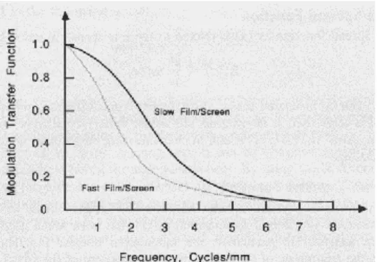
Figure 1-12: Example of line spread functions for two different kinds of film with different spatial resolutions. [3]

Modulation Transfer Function (MTF)

A common measure of system spatial resolution is the modulation transfer

function (MTF), which is defined as the magnitude of the spatial Fourier transform of the

line spread function: ( ) | ( ( ))| [3]

Figure 1-13: Sample MTF curves corresponding to the line spread functions shown in Figure 1-12. [3]

A sample MTF curve is displayed in Figure 1-13. Imaging systems suppress high spatial frequencies, in effect behaving as low pass filters. It is common to speak of the 10% MTF, or 5% MTF, which is the frequency in cycles/mm or line pairs/mm

corresponding with that value of MTF on the curve.

(46)

22

In order to use reconstructed CT volumes for diagnostic and treatment purposes as a proxy for actual patient volumes, it is necessary to assume that all relevant features in the patient appear in the CT image. Likewise, all features which appear in the CT image should correspond with physical features in the patient or imaging object. While this second assumption is usually correct, sometimes an imaging system will produce artificial structures, known as image artifacts. Some major causes of imaging artifacts include patient movement, beam hardening, radiation scatter, partial volume effects, and patient size exceeding the scanner field of view.

Figure 1-14: common CT image artifacts including (a) patient motion, (b) beam hardening, (c) partial volume, (d) metal implant (beam hardening), and (e) exceeding field of view. [5]

Patient Motion and Volume Inconsistency

(47)

x-23

ray imaging, when blurs appearing only in the moving regions. Because CT volume reconstruction is achieved by tracing linear x-ray paths backwards from the detector, motion blur in an isolated region of object space can lead to distortions and streaks in surrounding volumes in reconstruction space. Any type of temporal inconsistency in the imaging object space, whether patient motion or contrast agent concentration, can lead to distortion throughout portions of the reconstructed CT volume. We will revisit this topic again as it motivates the need for physiological motion gating in live animal imaging.

Beam Hardening

The artifact known as beam hardening arises from the assumption in CT

(48)

24

Both dark streaks from photon starvation and cupping artifacts are due to the polychromatic nature of the x-ray beam and the lack of accounting for this nature in traditional CT reconstruction. These artifacts could be eliminated entirely if CT imaging was performed with a monochromatic x-ray beam, or if the reconstruction algorithm took into account the energy dependence of attenuation. A common and straightforward fix which reduces the severity of beam hardening artifacts is to pre-filter the x-ray beam with a material, such as steel or aluminum, to reduce the number of low-energy photons in the x-ray beam before they enter the imaging object.

Partial Volume Effect

This class of image artifact applies especially to helical CT image acquisitions, but they are present though less severe in cone-beam CT. In partial volume artifacts, high contrast structures extend partially into adjacent slices. This results in a loss of sharpness in the feature edge along the z-direction and especially the appearance of shadows along the edge of these highly attenuating features. Partial volume effects can also occur within the x-y plane though usually less severely, since spatial resolution in-plane is better than along the z-axis. Partial volume effects, combined with beam hardening dark streaks, create characteristic image artifacts near the interfaces of high- and low-attenuation materials.

Field of View Artifacts

An essential assumption in CT reconstruction is that all portions of the imaging object are contained entirely within the field of view. If some portion of the object is outside of this field of view, then some x-ray paths will pass through it and the

(49)

25

reconstructed image, areas at the edge of the field of view and adjacent to the extra material will appear hyperdense compared with their true composition. When the amount of extra material outside the field of view is small, and the outer portions of the

reconstructed volume are not diagnostically crucial to view accurately, FOV artifacts are easy to interpret correctly and they are mostly harmless. However, if there are large amounts exterior material or if they are made of highly attenuating materials such as bone or metal, large streak artifacts can appear which obscure large areas of the reconstructed image.

As with beam hardening artifacts, a robust field of study exists to minimize the effect of field of view artifacts using special algorithms and corrections [Hsieh 2003]. This is an important problem to solve because of the increasing use of flat panel detectors in CT, and especially because the average patient size in the clinic has increased over time.

1.3 Pre-clinical high resolution CT (Micro-CT)

Due to the success of CT in human-scale and clinical imaging, this modality has now been applied to non-clinical imaging applications such as tissue samples, biopsies, and living animals. Micro-computed tomography (micro-CT or µ-CT) is the small-scale high resolution counterpart to the CT scanners used in hospitals, and the general

principles by which it operates are the same as discussed in the previous sections on CT. Ex-vivo and in-vitro imaging of biological samples using micro-CT is widely used for the same reasons clinical CT has become popular.

(50)

26

Mice in particular are heavily used in biomedical studies of disease because their genome is widely known, they reproduce quickly, and they are small and inexpensive to house. Researchers studying disease in mice require the same tools of diagnosis and disease monitoring as are available in the clinic, including optical and fluorescence imaging, ultrasound, magnetic resonance, and of course computed tomography.

There are special requirements for CT imaging of in-vitro and in-vivo small imaging, and the micro-CT scanner is adapted to these needs. In-vitro micro-CT and in-vivo small animal micro-CT are addressed separately in the following sections.

1.3.1 In-vitro Micro-CT

In in-vitro imaging, the primary demands are high contrast resolution and extremely high spatial resolution (between 5 and 50 microns) [5]. Thus, the smallest possible focal spot sizes are required of these scanners, generally at the expense of tube flux and therefore scanning speed. Long scan times are an annoyance for in-vitro imaging applications but not a serious problem, since the imaging objects are stationary and therefore will not move or change over the scan time, except perhaps for vibrational motion or evaporation of liquid in some samples. High radiation dose is also often relatively high but not considered an important factor since the imaging subject is not a living organism.

1.3.2 In-vivo Micro-CT

(51)

27

period of weeks or months, radiation dose needs to be minimized using the ALARA principle (As Low As Reasonably Possible). At the same time, scan timing is a crucial consideration, both because physiological processes of interest may evolve over the span of seconds or minutes, and also because rapid respiration and cardiac rates of mice (~120 and ~500 bpm, respectively) can introduce significant motion blur in images if not compensated for in some way. A comparison between the characteristics of in-vitro and in-vivo micro-CT scanning requirements is displayed in Table 1 [5].

In-vitro micro-CT In-vivo micro-CT

Focal spot size 1-30 µm 50-200 µm

x-ray power 1-30 W 10-300 W

Spatial resolution 5-100 µm 50-200 µm

Scan time 10-300 min 2s – 30min

Detector Flat panel Flat panel

Field of measurement 1-50 mm 30-100 mm

Dose Not important ALARA

Table 1-1: Comparison between in-vitro and in-vivo micro-CT parameters. [5]

Respiratory-Gated In-Vivo Micro-CT

The use of in-vivo micro-CT has been recently demonstrated for a variety of preclinical murine imaging applications [6, 7]. The high contrast between air and

(52)

28

matched to a particular phase of the respiratory or cardiac cycles (or both, depending upon the imaging application).

In the method of retrospective respiratory gating, x-ray projection images are acquired and each projection is sorted into a bin corresponding to a different phase of the respiratory cycle. Then during reconstruction, only projections corresponding to a single phase of respiration are used to generate the 3D CT image. To guarantee full angular coverage in the phase of interest, multiple rotations of the gantry are necessary. In extrinsic retrospective respiratory gating, a sensor must be used to monitor abdominal motion throughout the scan so that projections can be sorted into the correct phase bin [8, 13, 14]. In intrinsic retrospective gating, an algorithm is used to sort the projections into the correct phase based on visual inspection of the images themselves [15, 16]. Both intrinsic and extrinsic retrospective gating techniques have the benefit of easy

implementation and fast scan times but result in an increased radiation dose to the subject due to the resultant oversampling, potentially violating the ALARA principle.

(53)

29

on a single animal. Additionally, the process of mechanical ventilation has been shown to induce lung injury in otherwise previously healthy specimens [21 – 24]. These risks mean that forced breathing and breath-hold gating methods are not ideal for longitudinal

studies, particularly for sensitive disease models. Also, while external control of lung pressure and volume aids the imaging process, it can result in measures of tidal lung volumes and related values which are not accurate or physiologically relevant to the study.

A less invasive method of prospective gating permits free-breathing mice to be imaged by tracking respiratory chest motion of the animal with a pressure sensor or CCD camera and synchronizing x-ray pulses with a desired phase in the respiration cycle [25]; this general approach was used in my own work reported throughout the rest of this thesis. While the researcher does not have direct control of the physiological state of a free-breathing subject, it has been demonstrated that, in general, a healthy adult mouse under anesthesia and temperature control generally exhibits stable, quasi-periodic respiratory motion so that images of the thorax are blur-free [25]. The aforementioned technique has the drawback of increased scan times per CT image, but it keeps radiation dose to the subject low and does not require intubation (along with the associated risks). In order to achieve optimal results, one requires an x-ray source with good temporal resolution (100 ms or less to achieve blur-free respiration images [26]) and reliable information about the position of the subject’s lungs and abdomen at any given point of time.

Cardiac-Gated In-Vivo Micro-CT

(54)

30

times of 75.5 ms or less per slice are required to eliminate in-plane arterial motion blur in a typical patient with 50 bpm or greater cardiac rate [28]. To replicate the clinical

imaging technique with a murine subject of 350 bpm or greater while anesthetized, freezing motion of the heart within a single phase of the cardiac cycle requires imaging in less than 10 to 15 milliseconds. Thus successful cardiac gating requires each x-ray

projection exposure to persist for 15 ms or less in order to capture the diastolic phase without blur. Current micro-CT systems with conventional thermionic x-ray sources cannot easily produce such short yet uniform pulses non-periodically. Also, in cardiac-gated imaging there is no option for externally controlling heartbeats to coincide with pre-determined x-ray pulse intervals. Either prospective or retrospective gating techniques may be applied to micro-CT small animal cardiac imaging, with the same benefits and drawbacks discussed for respiratory gating.

For physiologically-gated small animal cardiac micro-CT imaging, the scanner’s x-ray source must have a small FSS, be capable of high flux for short pulse generation, yet also be capable of generating these pulses non-periodically and with almost