RADIAL DISTANCE WEIGHTED DISCRIMINATION
Jie Xiong
A dissertation submitted to the faculty of the University of North Carolina at Chapel Hill in partial fulfillment of the requirements for the degree of Doctor of Philosophy in the
Curriculum in Statistics
Chapel Hill 2015
c 2015 Jie Xiong
ABSTRACT
Jie Xiong: Radial Distance Weighted Discrimination (Under the direction of J. S. Marron and D. P. Dittmer)
ACKNOWLEDGEMENTS
TABLE OF CONTENTS
LIST OF TABLES . . . vii
LIST OF FIGURES . . . viii
1 THE MOTIVATION FOR RADIAL DWD . . . 1
2 BACKGROUND ON CLASSIFICATION METHODS . . . 12
3 RADIAL DWD . . . 28
3.1 Review linear DWD optimization . . . 28
3.2 Formulate Radial DWD optimization . . . 29
3.3 An iterative algorithm to numerically solve Radial DWD . . . 30
3.4 Miscellanies of Radial DWD optimization . . . 31
3.4.1 The dual problem . . . 32
3.4.2 An interpretation to the dual . . . 35
3.4.3 Weighting schemes . . . 37
4 RADIAL DWD ASYMPTOTICS . . . 39
4.1 Distance on the high dimensional simplex . . . 39
4.2 HDLSS geometric representation . . . 42
4.3 HDLSS geometric representation of Dirichlet distributions . . . 47
4.3.1 Representation of a single sample . . . 47
4.3.2 Representation of two samples . . . 51
5 SIMULATION ANALYSIS . . . 60
5.1 Simulation 1 . . . 61
5.2 Simulation 2 . . . 64
6 THE VIRUS HUNTING DATA ANALYSIS USING RADIAL DWD . . . 68
6.1 Introduce virus hunting dataset . . . 68
6.2 Radial DWD analysis: a single virus detection problem . . . 68
6.3 An automated pipeline using Radial DWD . . . 73
6.4 Multiple-virus detection and heatmap visualization . . . 75
6.4.1 Dataset 1: 52 sequenced samples . . . 75
6.4.2 Dataset 2: samples from a herpesvirus sequencing project . . . 77
6.4.3 Dataset 3: samples from 3 individual studies . . . 78
7 CONCLUSION . . . 85
APPENDIX A BIOLOGY AND BIOINFORMATICS BACKGROUND . . . 86
APPENDIX B THE PERFORMANCE OF RADIAL DWD PIPELINE . . . 91
B.1 Speed versus sensitivity . . . 91
B.2 Radial DWD and BLAST . . . 92
APPENDIX C MORE ON RADIAL DWD . . . 96
C.1 Discussion on the choice of “step length” parameter . . . 96
C.2 Radial DWD on unit sphere: a special case using “Geodesics” . . . 97
APPENDIX D DIRICHLET DISTRIBUTION . . . 100
APPENDIX E SIMULATION STUDY: A LINEAR EXAMPLE . . . 103
LIST OF TABLES
3.1 Weighting schemes for unequal costs . . . 38
3.2 Weighting schemes for biased sampling . . . 38
5.1 Parameterαused in simulation . . . 64
6.1 Target Herpesviruses . . . 69
6.2 Dataset 1, with 52 test samples . . . 75
LIST OF FIGURES
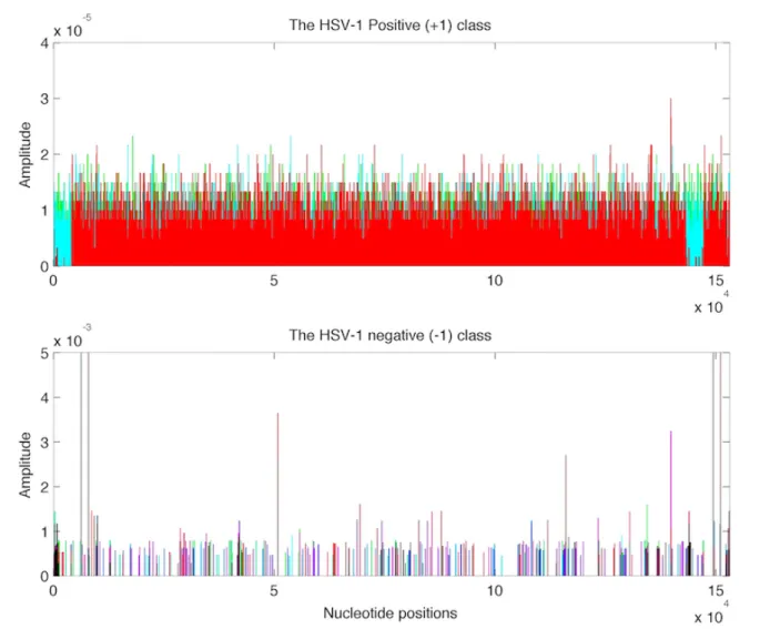
1.1 Overlaid plots of normalized coverage vectors from an HSV-1 example. . . 7
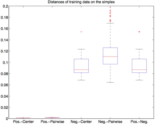
1.2 Distances of the training data on the simplex . . . 8
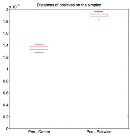
1.3 Distances of the positive data on the simplex. . . 9
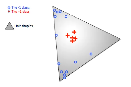
1.4 A simplified structure of the normalized coverage vectors . . . 10
2.1 An illustration of the idea of linear DWD. . . 19
2.2 A toy example comparing linear DWD with Radial DWD. . . 21
2.3 Training data on the unit simplex in the 3 dimensional space. . . 22
2.4 Linear DWD is not robust to the change of training set. . . 23
2.5 Radial DWD is robust to the change of training set. . . 24
2.6 The limiting behavior of Radial DWD by “pushing” the center to infinity. . . . 26
2.7 Brain tumor MRI may be classified using Radial DWD. . . 27
4.1 Relative relationships between the center of the Radial DWD sphere, and the means of two populations. . . 53
5.1 A toy example of the 3 dimensional Dirichlet density. . . 61
5.2 A simulated example illustrating the potential for improved performance of Radial DWD. . . 62
5.3 A boarder simulation study comparing Radial DWD with some competitors. . 65
6.1 A taxonomy tree of 21 reference Herpesviruses . . . 70
6.2 A real data example of an HSV1 classification problem. . . 72
6.3 The Radial DWD pipeline for a single-virus (HSV-1) detection. . . 74
6.4 Heatmap visualization of the Radial DWD score matrix for dataset 1. . . 80
6.6 Heatmap visualization for the LCLs samples. . . 82 6.7 Heatmap visualization for the Akata samples. . . 83 6.8 Heatmap visualization for the Human Burkitt0s Lymphoma (BL) samples. . . . 84 B.1 An EBV example comparing Radial DWD with BLAST. . . 94 C.1 An illustrate of the first order Taylor approximation. . . 97 D.1 The density of the symmetric three dimensional Dirichlet distributions with
various parametersα . . . 100 D.2 The density of the asymmetric three dimensional Dirichlet distributions with
various parametersα . . . 101 E.1 A simulation study illustrating the performance of Radial DWD in a linearly
CHAPTER 1: THE MOTIVATION FOR RADIAL DWD
We will discuss some useful virology background in this section and describe the virus hunting project which motivates our work. Viruses must replicate in living host cells. The replication and propagation of a given virus in a population is frequently (not always) mani-fest with the occurrence of an infectious disease that spreads between individuals (Wagner and Hewlett 2004 [1]). For example, infection with smallpox virus causes variola; infection with poliovirus can lead to paralytic polio. While variola and paralytic polio are both acute infec-tions, viral infections could also be chronic, like warts caused by papillomavirus and chronic lung infection caused by adenovirus. Some viruses, on the other hand, exhibit latency with episodic reactivation with ensuing milder symptoms of the original acute infection. In a latent infection, the viral genome is maintained in a specific cell type and does not actively replicate (Wagner and Hewlett 2004 [1]). Example viruses include human herpesviruses. At least five species of herpesviruses are extremely widespread among humans, including Human simplex virus (HSV), Varicella zoster virus (VZV or chicken pox), Epstein-Barr virus (EBV) and Cy-tomegalovirus (CMV). More than 90% of adults in the US have been infected with at least one of these, and a latent form of the virus remains in most people (Chayavichitsilp et al. 2009 [2], NCID 2006 [3]). Moreover, some viral infections have long incubation periods, like rabies, HIV-AIDS etc.
Detailed discussion of existing classification algorithms appears in Chapter 2.
The virus detection machine we designed, Radial DWD, will be shown to possess high sensitivity (or low false negative rate) and specificity (or low false positive rate) with robust performance (as discussed in Chapter 2). Before reviewing some existing methods, we would like to present virus detection as a classification problem. In the statistics and machine learn-ing literatures, a detection machine is called a classifier. A classifier takes virus negative and positive samples as a training set. Based on certain rules, the classifier computes a separating boundary such that the data points from positive and negative classes could be “best” separated. A future sample will be classified either to the virus positive or negative class using this sepa-rating boundary. Note that for our convenience, we will use the notations of +1 (-1) class and virus positive (or virus negative respectively) class interchangeably.
small number of anonymous donors. In order to overcome the potential sampling bias and to account for ethnicity, the 1000 Genomes Project [14] was carried out to generate three groups of geographically distinct reference sequences. In spite of this, we use Hg19 at this time. Note that a coverage vector can be seen as a data point in the Euclidean space so that we will use terminologies of positive/negativecoverage vectorsand positive/negativedata points interchangeably. Coverage vectors for testing cases will also be generated in the same way. Note that we exclude those samples whose reads do not align to the reference, or say we exclude zero coverage vectors, from the downstream classification analysis. Once we introduce the idea of Radial DWD in Chapter 2 and formulate the optimization of it in Section 3.2, it will be clear that ignoring these samples is equivalent to putting them at infinity. More information about how to randomly generate reads from DNA samplesin vitroand DNA alignment are included in the Appendix.
Thereafter, we train the classifier using coverage vectors from the virus homologies (the positives) versus the ones from Hg19 (the negatives). Each positive/negative training DNA sample is then numerically represented by a coverage vector which is of the same length as the reference virus. Additionally, increasing the total number of reads generated from a sample usually inflates entries in its coverage vector and vice versa. In many cases including our virus hunting project, the number of reads generated from samples differs. Meanwhile, in real sequencing experiments (in order to generate reads by using biological sequencing machines, not by the computational scheme described in Chapter 8), the total number of reads depends heavily on the experimental settings and the sequencing platform. The fact that we usually collect different numbers of reads for the samples is regarded as abench effecthere.
en-tries of the normalized vectors can be interpreted as proportions and all coverage vectors now have unit L1 norms, making them directly comparable to each other. Since the normalization technique described above projects coverage vectors to the unit simplex, we regard it as “unit simplex normalization”, see Section 4.1 for details.
A major statistical challenge in such a classification problem is called high dimension low sample size (HDLSS), where the dimension of the data space is much higher than the sample
size. For example, the human herpesvirus genomes are often of length 100 thousand to 200 thousand nucleotides (nts) long, which determine the dimension of the data space. However, usually the sample size, including both the positive and negative data points, is in the tens. Equivalently speaking, these samples are located in the Euclidean space of over 100 thousand dimensions or on a high dimensional unit simplex after being normalized! This characteristic will break down many traditional statistical inference methods, which motivates a need for new methods. The HDLSS problem will be further addressed in Chapter 2 and Chapter 4.
approximately the same, the data point is near the center. At the same time, the more zeros in a vector, the more close this data point is to one of the vertices of the unit simplex. In the extreme case when there is only one nonzero entry “1” in the vector, the data point is at a ver-tex. Note that entries of the positive (negative) data points are mostly nonzero (zero), making them locate near the center (vertices, respectively). Moreover, negatives usually locate among a very diverse set of vertices since the nonzero entries, or spikes, appear at different loci for each negative data point, determined by its common regions shared with the reference virus. This is a property of all virus detection problems, since the negative sequences are chosen to be genetically very different from the virus. The aligned reads (from the negatives to the virus sequence), on the other hand, are often short stretches of sequence which are of reduced com-plexity, i.e. repeats or single nucleotide (either A, C, T or G) runs. A simple yet insightful calculation of some typical distances on the unit simplex will appear in Section 4.1 which helps to better explain the geometry of these positive/negative data points.
Figure 1.1: Overlaid plot of 8 normalized data vectors of the HSV-1 positive (the +1) class is shown in the top panel by different colors; the bottom panel shows the overlaid plot of 24 data vectors from the HSV-1 negative (the -1) class. The overall entries of the +1 data vectors are relatively small (see the vertical axis labels) and have relatively comparable amplitudes. Nonzero entries of the -1 data vectors are sparse and with large amplitudes (over 100 times larger than that of the positive samples). Additionally, differently colored peaks of the -1 data vectors show that the -1 class is located near quite divergent vertices of the unit simplex. Note that if we keep the same range of y-axis in plotting the positive data vectors as in plotting the negative data vectors, one can see almost nothing since the amplitudes of the former ones are much smaller than the latter ones.
Figure 1.2: Boxplots to show some typical distances of the training data from Figure 1.1. Remember that the data points are located on the simplex. The boxplots labeled ‘Pos.(Neg.)-Center” shows the pairwise distances between the positives (negatives) and the overall center of the simplex; the boxplot labeled “Pos.(Neg.)-Pairwise” shows the pairwise distances within the positive(negative) data points; the boxplot labeled “Pos.-Neg.” shows the pairwise distances between the positives and the negatives. It can be seen from the “Neg.-Pairwise” boxplot that the negatives are quite diversified and 14 out of 24 are above the upper whisker.
Figure 1.3 provides an easier illustration of the distances related to the positive data points, which is a zoomed-in version of Figure 1.2 by considering only the Center” and “Pos.-Pairwise” boxplots. It shows that the pairwise distances among the positives are larger than their distances to the center, approximately by a factor of√2. It follows that when we consider the vector pointing from the center of the simplex to each positive data point, those vectors are approximately orthogonal to each other.
Figure 1.3: Boxplots show distances between the positives and the overall center of the sim-plex, as well as the pairwise distances among the positives.
located near different vertices, surrounding the center from diverse directions.
Figure 1.4: A simplified example of normalized data vectors of the positive (+1 class) data (red plus signs) and the negative (-1 class) data points(blue circles). The unit simplex is shown as the gray triangle. Because there are many zeros in the -1 data vectors, they typically locate at the vertices of the unit simplex while the positives are more close to the center.
It will be seen in Chapter 2 that many linear classifiers have been designed for HDLSS classification. However, the special geometry of virus hunting datasets motivates the develop-ment of classifiers to explicitly deal with nonlinearity among the training set (the positives near center, surrounded by the negatives distributed around different vertices of the unit simplex). Such a development is given in Chapter 2 where we propose to fit a separating (hyper)sphere by using Radial DWD, to separate the positive and negative data points, in favor of putting the positives inside and negatives outside of the (hyper)sphere.
CHAPTER 2: BACKGROUND ON CLASSIFICATION METHODS
Classification is a supervised learning problem of assigning class labels to new observations on the basis of given training data, of which the class labels are known. Various types of methods or classifiers have been proposed to better “learn” from the training data. It is also well known that the performance of classifiers depends heavily on the underlying data structure so that no single method is best for all circumstances. Good references to the classification include Hand (1981) [16], MacLachlan (1992) [17], Gordan (1999) [18], Hastie, Tibshirani and Friedman (2009) [19], Duda, Hart and Stork (2006) [20]. We would like to give an overview of the popular classification methods and discuss their HDLSS performances, especially for virus hunting data analysis. Good references on HDLSS data analysis and challenges include Hall, Marron and Neeman 2005 [21], Liu et. al 2008 [22], Jung and Marron 2009 [23], Jiang, Marron and Jiang 2009 [24].
this paper, when we consider the classification with more than 2 classes (e.g.K>2), the class labels are coded as the integers ranging from 1 to K; in case of binary classification (e.g. K=2) the class labels are coded as -1 (for negative class) and +1 (for positive class). Note that, throughout the paper, we will use terminologies of features and covariates interchange-ably while they actually both mean the measurements of the observations. For convenience of visualization, we will also discuss the separating boundary computed by each classification method.
We first introduce binary linear classifiers. A binary linear classifier inRdcan be expressed as f(x) = wTx + b, where the d-column vector w is the normal vector of the separating hyperplane and the scalerb is called the shift or location parameter. Definesign(f(x))as the class label associated with measurementx. By projecting data onto the normal vector, we hope that the observations from different classes are well separated. Various methods have been proposed to “best” estimate the normal vectors and the shift parameters under various criteria. Among the most well known ones include the Centroid or Mean Difference method (Scholkopf¨
and Smola 2002 [28]), the Linear Discriminant Analysis method (Fisher 1936 [27]) and the Naïve Bayes rule (Domingos and Pazzani 1997 [29], Hand and Yu 2001 [30]).
Marron et al. (2009) [24] proposed “RCME”, a robust centroid based classification method by replacing the class means with Hubers’L1 M-estimate (Huber 1981 [32]) and showed its ro-bustness against non-Gaussian distributions.
The Linear Discriminant Analysis (LDA) and the Naïve Bayes rule (NB) can both be for-mulated through maximizing the “class posterior densities” given observations, assuming ob-servations are generated from the multivariate Gaussian distributions. However, LDA and NB differ in an important way in terms of estimation of the underlying data variance-covariance structure.
still needs to be considered.
On the other side, the Naïve Bayes (NB) rule maximizes the class posterior densities assum-ing that each of the class densities is the product of marginal densities or equivalently assumes conditional independence of the features in each class (Domingos and Pazzani 1997 [29]). It has long been recognized that in case of HDLSS classification, rules that assume independence between covariates (or features) may outperform the classifiers trying to estimate the covari-ance structure (see Bickel and Levina 2004 [34], Domingos and Pazzani 1997 [29], Lewis 1998 [35], Levina 2002 [36], Dudoit et al. 2002 [37]). Naïve Bayes sometimes outperforms many sophisticated methods. This is true as the independence assumption guarantees a much smaller set of covariance parameters to be estimated which reduces noise and meanwhile the approximating covariance matrix could well capture the data covariance structure.
Notice that applying LDA involves inverting the whole covariance matrix while applying NB involves inverting a diagonal approximating covariance matrix. Under HDLSS settings, due to the singularity of the sample covariance matrix, the exact inverse is unavailable. One could use the generalized inverse instead, such as the Moore Penrose inverse (Moore 1920 [38]; Penrose 1955 [39]). Generalization of the above linear classifiers to HDLSS cases is then computable but this leads to poor performance as shown in Ahn and Marron (2010) [40].
tend to be far away from each other, causing the upper bound of asymptotic errors being not valid anymore (Friedman 1994 [43]). Hastie and Tibshirani (1996) [44] proposed the so-called Discriminant Adaptive Nearest-Neighbor (DANN) and extend K-NN to the high dimensional classification, assuming the class probabilities change only along a low-dimensional subspace. Similar ideas can be found in Short and Fukunaga (1980) [45], Myles and Hand (1990) [46].
Another approach to classification is through regression. The extension of the Linear Re-gression is natural. Suppose we haventraining data points of which the class labels are known a priori. Let an vector of class labels be the responseY and denote itsith entry asYi, i=1...n. SupposeK is the number of classes, we usually code the class labels so thatYi ∈ {1,2, ..K}. LetXi ∈ Rd be the input feature vector of theith training data points and Yi = k iff i ∈ kth class, k=1...K. The Linear Regression classifier, trained by regressingY onX, gives a linear (or piece-wise linear in the case K>2) separation hyperplane by assigning new observations to class k if the fitted values of the observations are closest to k (among 1...K), see Hastie, Tibshirani and Friedman (2009) [19] whereY is coded as a matrix of indicators. Although the Linear Regression classifier is simple to formulate and compute, because of the rigid model assumption of linearity, classes can be masked by each other whenKis big. It is worth noting that the basis expansion of input features, e.g. by including higher order polynomial terms and interaction terms of covariates for instance, one could significantly improve the linear models’ flexibility. By coupling with a basis expansion and doing classification in an enlarged feature space, one could get a much more flexible classification boundary after mapping the separating hyperplane from the enlarged space back to the original one.
To deal with binary linear classification, some other methods directly optimize in order to find the “best” linear separating boundaries (or hyperplanes). One of the most famous methods of this type is Support Vector Machine (SVM). SVM tries to maximize the minimum distance between classes (Burges 1988 [56]; Cristianini and Shawe-Taylor 2000 [57]). Although SVM is intuitively pleasant and relatively easy to solve numerically, Marron et al. 2007 [58] observed that in high dimensions it may be subject to an issue called “data piling” where data points could have identical projections in the SVM normal direction within each class. Later Ahn and Marron (2010) [40] discovered the “Maximal data piling direction” (MPD) and showed when the dimension of the feature space is larger than the sample size one could usually find a direction that gives perfect data piling. Directions with data piling overfit the training data and may suffer from low generalizability (Marron et al. 2007 [58]).
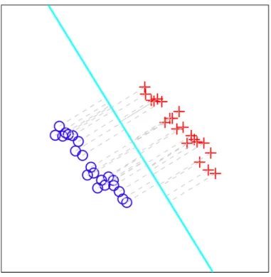
To alleviate the data piling and therefore improve generalizability, Marron et al. (2007) [58] invented a binary linear classification method called Distance Weighted Discrimination (DWD). DWD tries to find a separating hyperplane by minimizing the sum of inverse distances from each data point to the separating hyperplane, as illustrated in Figure 2.1. The optimization problem of DWD can be formulated into a Second Order Cone Program (or SOCP, see Alizadeh and Goldfarb 2003 [59] for a good review) and numerically solved by a recently developed infeasible point algorithm called SDPT3 (Tutuncu, Toh, Todd 2001 [60]).
Figure 2.1: A toy example illustrating the idea of linear Distance Weighted Discrimination. Class +1 (positive) data points are shown as red pluses while Class -1 (negative) data shown as blue circles. The separating hyperplane is shown as the cyan line. Each data can be projected onto the hyperplane through the grey dashed line segments and the length of those segments are distances from the samples to the separating hyperplane.
However, for virus hunting data analysis, even if the training classes are linearly separable, linear classifiers are not the best option. It will be shown by simulation and real data in Chapter 5 and 6 that linear classifiers present high classification error. In case of a very divergent negative training set where negatives tend to locate near many distinct vertices of the unit simplex, it is more natural to consider some more flexible nonlinear separating boundaries.
is Shawe-Taylor and Cristianini 2004 [72]. However, it was noted by El Karoui 2007 [73] that in HDLSS settings, linear SVM and DWD often performs better than their nonlinear kernel extensions. This may happen because of kernel methodsoverfitthe training data.
Being aware of the limitation of the linear and kernel classifiers, we propose a novel method, Radial DWD, to fit a hypersphere, a sphere in a high dimensional space parameterized by its center and radius, as the classification boundary. To be more specific, we want to fit a hypersphere so that data points from the positive class tend to lie inside while data points from the negative class tend to lie outside. Simulations and real data will be presented to show the advantages of Radial DWD over linear competitors and kernel methods in Chapter 5 and Chapter 6.
Radial DWD mimics the rationale behind linear DWD while substituting the conventional “Euclidean distance” with “radial distance”, see Figure 2.2 for a 2-dimensional example, where Radial DWD tries to find a separating sphere that minimizes the sum inverse of “radial dis-tances” from each data point to the separating hypersphere. Note that in Figure 2.2, training data are shown by red plus signs (the positives) and blue circles (the negatives) while the cor-responding separating boundary is shown in cyan. The radial distances are the lengths of the grey dashed line segments, shown in the right panel in Figure 2.2.
Figure 2.2: A toy example comparing the rationale behind linear DWD and Radial DWD. In the left panel, DWD separating boundary is linear, shown by a cyan line; in the right panel, the separating boundary is a sphere, shown by a dashed cyan circle. In both panels, the distances to separating boundaries (or residuals) are the lengths of grey dashed line segments connecting the data points to the separating boundary. We regard those distances in Radial DWD as “radial distances”.
separating boundary or the jitter plot.
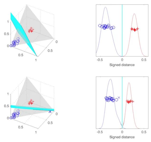
Figure 2.3:A simple 3 dimensional example showing that the training set is located on the unit simplex, reds are positive and they are near the center, blues are negative and they are near a vertex.
Figure 2.4:A simple 3 dimensional example showing linear DWD is not robust to the change of training set. The upper left panel shows the linear DWD separating plane (cyan) trained by reds versus blues; the upper right panel shows a jitter plot of the signed distances of the training data points to the separating plane in x axis (and y axis shows random heights to separate data points, for a better 1 dimensional view), kernel densities are given as well; the lower panels are similar except that we add one more negative training data point (blue cross) near another vertex and re-train linear DWD using reds versus blues, including the new data point. One could observe a drastic change in the separating plane by comparing the upper and lower left panels; additionally, the distance from the positive data points to the separating plane shrink as well by looking at the jitter plot and kernel densities in the lower right panel.
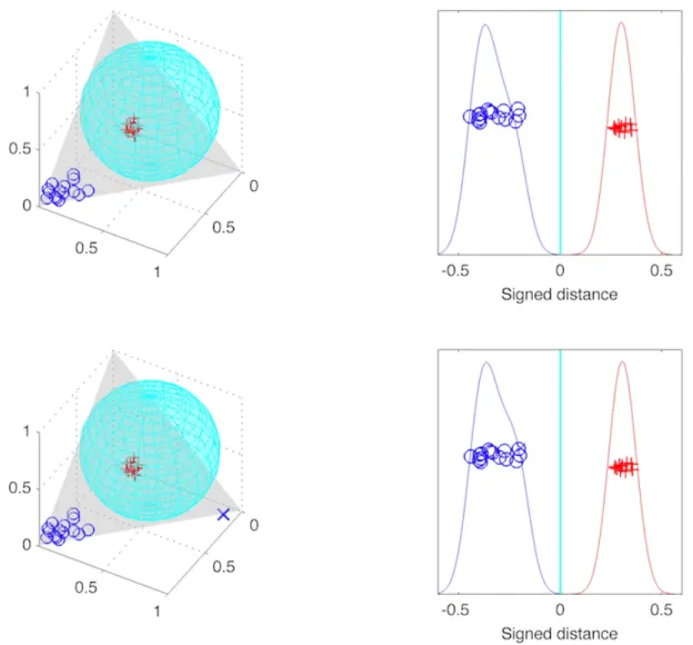
Figure 2.5: A simple 3 dimensional example showing Radial DWD is more robust to the change of training set. The upper left panel shows the Radial DWD separating sphere (cyan) trained by reds versus blues, in the upper right panel, a jitter plot with kernel densities is given and the x-axis shows the distances of the training data points to the separating sphere (the y axis shows random heights to separate data points, for a better 1 dimensional view); lower panels are similar except that we add one more negative training data point (blue cross) and re-train the Radial DWD including the new data point. One could observe that the separating sphere remains stable by comparing the left two panels; additionally, the distance from the training data points to the separating plane are stable as well.
hy-perplane. In Figure 2.6, we show a simple 2-dimensional toy example when we “push” the center of separating sphere further away from the training data along the direction of linear DWD normal vector (the vector that is orthogonal to the DWD separating hyperplane, pointing to the positive data) to the infinity. In the upper left panel in Figure 2.6, we train both linear and Radial DWD using red pluses versus blue circles. The separating boundary is either depicted as a black dashed line (for linear DWD) or a cyan circle (for Radial DWD). Suppose the normal vector of linear DWD hyperplane is w ∈ R2, the center of Radial DWD sphere is O ∈ R2
and we attempt to moveO further away from the data by defining the center as O+λwand makeλ → ∞. Note that each time when we attempt to increase λ, Radial DWD calculates the separating sphere by optimizing its radius only, with its center fixed atO+λw. Asλgets bigger, the separating boundary given by Radial DWD appears more and more linear near the data points and gradually the 2 separating boundaries (showed by cyan and black) converge.
CHAPTER 3: RADIAL DWD
3.1 Review linear DWD optimization
Since Radial DWD is a generalization of the conventional linear DWD, it is useful to give an overview of optimization details associated with the latter one. First of all, let us set the notations to be used. The training set consists of n d-vector xi together with corresponding class labels yi ∈ {−1,+1}, i = 1...n. We let X denote the d × n matrix whose columns are xi. Let n+ = Σni=1I{yi=+1} andn− = Σni=1I{yi=−1} = n−n+ be the sample size of the
positive class and the negative class respectively. To simplify the notations, we use Y as a n×n diagonal matrix withyi as theith diagonal entry. Denotew ∈ Rd as the normal vector of the separating hyperplane and β ∈ R as the shift parameter. The residual of the ith data point isr¯i = yi(xTi w+β), or in matrix-vector notation r¯= Y(XTw+βe)wheree ∈ Rnis a column vector of1s. To incorporate inseparable cases, we add a term called “slack variable” in order to account for misclassification, denote byε ∈ Rn+ as in Burges (1998) [56], Marron et al. (2007) [58]. Thereafter, Marron et al. (2007) [58] define the perturbed residuals to be r=Y(XTw+βe) +ε. The linear DWD minimizes the sum of the reciprocals of ther
i plus a penalty term of the classification error:
M inr,w,β,ε X i
1
ri
+CeTε (3.1)
s.t. r=Y(XTw+βe) +, wTw≤1, r≥0, ε≥0 (3.2)
(SOCP) and solved by SDPT3, a primal-dual infeasible path following algorithm developed by Tutuncu, Toh, Todd, 2001 [60].
3.2 Formulate Radial DWD optimization
Now let us turn to the optimization problem associated with Radial DWD. Note that we will write each term explicitly for now instead of in a matrix form. We still minimize the sum of reciprocals of the residuals penalized by the augmented sum of classification error. But now we define the residualsriin a different way: ri =yi(R− kxi−Ok2), whereyiandxiare the same as appear in Section 3.1,R ∈ R+is the radius and O ∈ Rdis the center of separating sphere, k.k2represents the Euclidean norm. Therefore as defined,riis the signed distance between the data pointxi to the separating hypersphere with smallest absolute value. By requiring ri ≥ 0 we are actually in favor of putting positive data points (from class +1) inside the separating sphere while putting negative data points (from class -1) outside. As for linear DWD, we re-define the residuals by adding the slack variable: ri =yi(R− kxi −Ok2) +εi. Therefore the optimization problem to be solved looks as follows:
M inr,O,R,ε
X
i
1
ri
+CeTε (3.3)
s.t. ri =yi(R− kxi−Ok2) +εi, i= 1...n (3.4)
R ≥0, r≥0, ε≥0 (3.5)
whereris a vector ofri,εis vector ofεi. Similarly,Cis a tuning parameter to be determined, a largeCpenalizes more on classification error and vice versa. Following Marron et al. (2007) [58], we linearize the objective function by definingρi = (ri +r1
i)/2andσi = ( 1
ri −ri)/2, so
that r1
i =ρi+σi,ri =ρi −σi. Equivalently we could reformulate the problem as:
M inρ,σ,O,R,ε
X
i
(ρi+σi) +CeTε (3.6)
s.t. ρi−σi =yi(R−di) +εi, di =kxi−Ok2i= 1...n (3.7)
ρ2i −σi2 = 1, ρi−σi ≥0, i= 1...n, (3.8)
Additionally, we relax the constraints
{ρ2i −σ2i = 1, ρi−σi ≥0, i= 1...n} (3.10)
to the second order cone (SOC) constraint
{(ρi, σi,1)∈S3, i= 1...n}, (3.11)
where the SOC of dimensionkis defined as
Sk ={(ς;µ)∈Rk :ς ≥ kµk2}. (3.12)
It is not hard to show when the 2 classes are separable by using a hypersphere, this relaxation will not change the optimal solution. Substitute with the SOC constraints, the optimization problem becomes:
M inρ,σ,O,R,ε
X
i
(ρi+σi) +CeTε (3.13)
s.t. ρi−σi =yi(R−di) +εi, di =kxi−Ok2i= 1...n (3.14) (ρi, σi,1)∈S3, i= 1..n, (3.15)
R≥0, ε≥0 (3.16)
This is almost a Second Order Cone Program (SOCP) except that the equality constraints
{di =kxi−Ok2, i= 1..n} (3.17)
are nonlinear (which also makes the problem non-convex). We will use the first order Taylor expansion iteratively to approximate the nonlinear equalities by linear ones, which will be detailed in the following algorithm in Section 3.3.
3.3 An iterative algorithm to numerically solve Radial DWD
Initialization (Step 0):
Choose an initial center of the separating hypersphere and denote it as O0 (e.g. the mean or the coordinate-wise median of the +1 class training data), let the initial objective value be Obj0 =−1(an arbitrary negative number).
The iteration at Stepk: k≥1
Apply the first order Taylor expansion ondiaroundOk−1, that is, di =kxi−Ok2 ≈
p
(xi−Ok−1)T(xi−Ok−1) + (∇
O=Ok−1kxi−Ok2)T(O−Ok−1)
(3.18)
=kxi−Ok−1k2 −
(xi−Ok−1)T kxi−Ok−1k2
(O−Ok−1) := d0i (3.19)
Notice thatd0i is a linear function ofO. By substitutingdi withd0i, the optimization becomes a valid SOCP and could be solved forOkandRkusing SDPT3. LetObjkbe the current objective value at stepk.
Stop: if|Objk−Objk−1|< , whereis a predetermined precision parameter.
Note that at each step k, in order to well approximate the nonlinear terms by using the first order Taylor expansion, we further confine Ok in a neighborhood of Ok−1 (the solution computed from the previous step) by adding one more constraint to the original optimization: kOk−Ok−1k
2 ≤δk, whereδk ∈R+is called thestep lengthparameter. A smallδkguarantees the precision of Taylor expansion but may slow down the whole procedure. This additional constraint is actually a SOC constraint (δk, Ok−Ok−1) ∈ Sd+1 so that we still end up with a valid SOCP at stepk. In our current data analysis, we choose = 10−4 andδ
k = 10−4. The choice of penaltyCwill be discussed in Section 3.4.1.
3.4 Miscellanies of Radial DWD optimization
3.4.1 The dual problem
To gain more insights of Radial DWD, it is useful to give the dual formulation of the SOCP at each stepk. Let
wik−1 = (xi−O
k−1)
kxi−Ok−1k2
, (3.20)
dk−i 1 =p(xi−Ok−1)T(xi−Ok−1). (3.21)
and they are functions ofxi. After some algebra, we could come up with the dual formulation associated with the primal SOCP (as in (3.13) to (3.16) withdi replaced byd
0
i) at stepk: M axz
X
i
yizidk−i 1+δk(−k
X
i
yiziwk−i 1k2) + 2
X
i √
zi (3.22)
s.t.0≤zi ≤C, i= 1..n, (3.23)
Σiyizi ≤0 (3.24)
It is neat to put the primal and dual problem in more compact matrix forms. First of all, let us again clarify the notations, Y denotes the diagonal matrix with yi on the diagonal, y is the n vector of class labelyi. Denoteea vector of 1s,ρandσthen-vectors withρiandσias entries,ε the vector of classification errors,Wk−1 = (wk−1 1, ..., wnk−1)∈Rd×nwithw
k−1
i defined above. Besides, let4k−O 1 =O−Ok−1 anddk−1 = (dk−1 1, ..., dk−n 1)T ∈Rnso that:
(Primal) M inρ,σ,4k−1
O ,R,ε Ce
Tε+eTρ+eTσ
(3.25) s.t. σ−ρ+Ry+Y Wk−T 14Ok−1+ε=Y dk−1, (3.26) (δk,4k−O 1)∈Sd+1, (ρi, σi,1)∈S3, i= 1..n, (3.27)
R ≥0, , ε≥0 (3.28)
(Dual) M axz dTk−1Y z+δk(−kWk−1Y zk) + 2eT
√
z (3.29)
s.t.0≤z ≤Ce, i= 1..n, (3.30)
yTz ≤0 (3.31)
It is not hard to show the existence of strict feasible solutions to both the primal and the dual problems. Since the primal and the dual are convex so that the solution of following optimality conditions are guaranteed to be optimal, equivalently speaking, the following equations are sufficient and necessary optimality conditions.
σ−ρ+Ry+Y Wk−T 14k−1
O +ε=Y dk−1, (3.32)
0< z ≤Ce, ε≥0,(Ce−z)Tε= 0, (3.33)
R≥0, yTz ≤0, R(yTz) = 0 (3.34)
EitherWk−1Y z = 0andkO−Ok−1k ≤δk, (3.35) OrkO−Ok−1k=δk(Wk−1Y z)/kWk−1Y zk, (3.36)
ρi = zi+ 1 2√zi
σi = zi−1 2√zi
for alli= 1..n (3.37)
It is important to address that in most cases the optimal radius is nonzero. Suppose we fix the center of separating sphere to beO so thatdi >0is true for all i (which is the case whenC is large and the 2 classes are separable). LetP andN denote the index set for the positive (+1) class and negative (-1) class respectively. From the original formulation of primal problem, when the radius is set to zero, the objective function can be written as:
X
i∈P
( 1
εi−di +Cεi) +
X
i∈N
1
di (3.38)
Sincedis are fixed numbers as the center is fixed, by maximizing (3.38) with respective toεi the primal objective value can be written as
Pobj = Σi∈P(2 √
C+Cdi) + Σi∈N
1
di
(3.39)
forR =φas:
Σi∈P(
1
φ+ε0i−di
+Cε0i) + Σi∈N(
1
di−φ
) (3.40)
≥Σi∈P(2 √
C+Cdi−Cφ) + Σi∈N(
1
di−φ
) (3.41)
≈Σi∈P(2 √
C+Cdi−Cφ) + Σi∈N(
1 di + φ d2 i ) (3.42)
= Σi∈P(2 √
C+Cdi) + Σi∈N(
1
di
) +Cφ(Σi∈N(
1
Cd2
i
)−Σi∈P1) (3.43)
=PObj+Cφ(Σi∈N(
1
Cd2
i
)−Σi∈P1) (3.44)
=PObj0 (3.45)
Since
( 1
di−φ
) = 1
di
(1− φ di
)−1 ≈ 1 di
(1 + φ
di
) = 1
di
+ φ
d2
i
. (3.46)
Obviously,PObj0 < PObjiff
(Σi∈N(
1
Cd2
i
)−Σi∈P1)<0, (3.47)
which is true by choosing a largeC. Often the case for virus hunting, the number of members in the negative class is larger than that of the positive class so that Cd2
i > n−
n+ for i ∈ N is
sufficient to guarantee a nonzero radius at optima. Suppose this is true, we can modify the third line of optimality conditions as: yTz = 0, R > 0. The requirement of positive radius is conceptually pleasant and this will be shown important in Section 3.4.2 where we discuss an interpretation of the Radial DWD dual problem. Moreover, the conditionCd2
i > n−
n+ fori∈N
could be a candidate criterion for choosing the parameterC.
we solve the reduced problem. BecauseQis orthonormal, the original and the reduced prob-lem have the same objective values: suppose(ρ, σ, O, R, ε) is primal feasible to the reduced problem, it is easy to show(ρ, σ, QO, R, ε)is feasible to original primal problem. Notice that O ∈Rn,QO ∈Rdand the following hold
dk−i 1 =p(xi−Ok−1)T(xi−Ok−1) (3.48) =p(Qxi−QOk−1)T(Qxi−QOk−1) (3.49) wi,k−T 1(O−Ok−1) = (Qwi,k−1)T(QO−QOk−1) (3.50)
k4k−O 1k2 =kO−Ok−1k2 =kQO−QOk−1k2 (3.51)
Sincewi,k−1is also computed from the reduced problem so thatwi,k−1 ∈Rnand
Qwi,k−1 =
(Qxi−QOk−1) kxi−Ok−1)k2
= (Qxi−QO
k−1)
kQxi −QOk−1k2
∈Rd. (3.52)
Thus all terms that depend onX stay the same between the original and reduced problem so that a reduced feasible solution could be easily transformed into an original feasible solution without changing the objective value. After all, the 2 problems are equivalent.
3.4.2 An interpretation to the dual
Let us give an interpretation to the dual problem. Assume that the two classes are separable with a “proper” sphere which has nonzero radius, therefore R > 0 and yTz = 0 are true at optima. Moreover, yTz = 0 implies eT
+z+ = eT−z−, where z+(z−) is the subvector of z
corresponding to the positive (negative) points ande+(e−)the corresponding vector of ones. It
makes sense to scalezsuch thateT+z+=eT−z−= 1. We can writezin the dual problem asηz∗, whereηis a positive scaler andz∗satisfies the additional scaling condition. By maximizing the dual objective function with respective toηfor a fixedz, we find if
−dT k−1Y z
∗
+δk(kWk−1Y z∗k)>0 (3.53)
Then
p
ˆ
η= e
T√z∗
Equivalently the dual objective function becomes:
M axz∗
(eT√z∗)2
−dT
k−1Y z∗+δk(kWk−1Y z∗k)
(3.55)
Moreover we have
dTk−1Y z∗−δk(kWk−1Y z∗k) (3.56)
= (Σi∈Pdk−i 1zi∗−Σi∈Ndik−1zi∗)−δkkΣi∈P
xi−Ok−1 dk−i 1 z
∗
i −Σi∈N
xi−Ok−1 dk−i 1 z
∗
ik (3.57)
Since Σi∈Pzi∗ = 1 with z∗i ≥ 0, Σi∈Pdk−i 1zi∗ is a convex combination of dk−i 1 and it may be interpreted as anaverage distancefrom the current center of the separating sphere to all the positive data points, similar forΣi∈Ndk−i 1zi∗. In the case when two classes are separable with R > 0, the positive (negatives) will be locating inside (outside) the separating sphere so that the average distance of negative points are larger than that of the positive points:
Σi∈Pdk−i 1z ∗
i −Σi∈Ndk−i 1z ∗
i <0 or −d T k−1Y z
∗ >0
(3.58)
From the above observation, (3.53) is true when two classes are separable. Meanwhile, (3.53) is a measure of separability of the 2 classes and the bigger the absolute value, the bigger the separability. Additionally,wk−i 1 = xi−Ok−1
dki−1 is a vector of unit Euclidean norm pointing from the current center to each data point. Suppose we define thecentroidof the positive (negative) class as the convex combination ofwik−1,i∈P(orNrespectively) under weightszi∗s, therefore
Σi∈N
xi−Ok−1 dk−i 1 z
∗
i −Σi∈P
xi−Ok−1 dk−i 1 z
∗
i (3.59)
3.4.3 Weighting schemes
Note that in some situations, the proportions of the 2 classes in the dataset may not be able to reflect the real proportions in a target population due to sampling bias, or the 2 classes are extremely unbalanced. The separating boundary tends to be closer to the class with smaller training sample size. Qiao et al.(2010)[65] developed a weighting scheme and we follow the same line to set up the weights we use in Radial DWD. Suppose we need to optimize the following objective function:
X
i
w(yi){
1
ri
+CeTε} (3.60)
subject to the same set of constraints defined before. Note thatw(yi)is theweightassociated with the ith training data point and it only depends on the class label andw(y
i) = 1 in our previous setups.
Qiao et al.(2010) [65] also mentioned that in some applications, it is more desirable to use different costs for different types of misclassification, say, classifying a positive sample as negative may be more serious than classifying a negative sample to positive. This may be true when we do virus hunting since in order to find new viruses whose genetic information is diluted in tons of host DNAs, the diagnosis machine may be tuned to be sensitive so that the false negative is more serious than the false-positive. Therefore, Overall Misclassification (OM) criterion and Mean Within Group Error (MWGE) criterion are developed to assess the misclassification, see Qiao and Liu 2009 [66]. Based on OM and MWGE, they proposed the corresponding weighting scheme in Table 3.1 and 3.2. Table 3.1 shows the weighting scheme to adjust for the unequal costs and Table 3.2 is the weighting scheme for biased sampling. Note that c+(c−)
is the false-positive (false-negative) cost, π+(π−)
is the class probability of the positive (negative) class in the population; π+
s(π −
Criterion OM MWGE w(+1) c+ c−
π+
w(-1) c− c+ π−
Table 3.1: Weighting schemes for unequal costs
Criterion OM MWGE w(+1) c−ππ++
s
c− πs+
w(-1) c+π− πs−
c+
πs−
Table 3.2:Weighting schemes for biased sampling
In our virus hunting data analysis, currently we use weighting scheme in order to adjust for unbalanced training sets so that the weights in (3.60) are:
w(+1) = n−
n++n−
;w(−1) = n+
n++n−
. (3.61)
CHAPTER 4: RADIAL DWD ASYMPTOTICS
In this chapter, we are going to examine the d asymptotics of HDLSS data, where the dimension of the data spacedgoes to infinity and the sample sizenstays fixed (see Hall, Marron and Neeman 2005 [21], Ahn 2006 [67] and Qiao et al. (2010)[65]). Section 4.1 computes some distances on the high dimensional simplex. Section 4.2 studies the geometry of HDLSS data and shows that the (scaled) pairwise distances between the data vectors become a constant in the limit. The HDLSS geometric representation for the Dirichlet distributions is discussed in Section 4.3. Section 4.4 connects this HDLSS geometry with Radial DWD and discusses the asymptotic behavior of Radial DWD.
4.1 Distance on the high dimensional simplex
For data in the non-negative orthant, Rd
+ = {x = (x1, ..., xd)T : x1 ≥ 0, ...xd ≥ 0}, consider the following scale normalization that map nonzero data points to the unit simplex S ={x∈Rd
+ : Σdj=1xj = 1}. Supposex∈Rd+\{0}, the following operation defines the “unit
simplex” normalization:
Ps(x) = x
Σd j=1xj
(4.1)
Next explore the structure of this data space as the dimension grows, i.e. in the limd→∞, using the notations off ace andf ace center. To define these, first define the unit vectors,ej to have a 1 in the jth entry and 0 elsewhere for j = 1, ..., d. Let I denote any index set of cardinalitym, i.e. I ⊆ {1, ..., d},#(I) = m. Then take the m−f ace indexed byI, denote byF(I)to be the linear span of{ej : j ∈I}. Each such face has a center. For I denoting the index set of anmface, the face center ofF(I)a vector whosejthentry is 1
Because the faces are disjoint, we must havem+n ≤d. The distance between the respective face centers is:
ds(µs(I), µs(J)) ={m×(
1
m)
2+n×(1
n)
2}1/2 = ( 1
m +
1
n)
1/2
(4.2)
A simple special case is both1−f aces, m = n = 1, where ds(µs(I), µs(J)) = √
2, which is consistent with the simplest version of the Pythagorean theorem. An important case is both
(d/2)−f aces,m=n=d/2, where
ds(µs(I), µs(J)) ={(
2
d) + (
2
d)}
1/2 = 2d−1/2 (4.3)
Also of interest is the distance from a unit direction (a1−f ace) to the center of the disjoint
(d−1)−f aces,
ds(µs(I), µs(J)) = {1 + (
1
d−1)}
1/2 = 1 +O(d−1)
(4.4)
The main conclusion here is that them−f aceandn−f aceare close to each other if bothm andnare big and are far apart ifmand/ornbecome(s) small.
Next consider some distances to the overall center point of S. As above, letF(I)denote a givenm−f ace, i.e. #(I) = m. First denote the overall center asµs = (1d, ...,1d)T. Note that
ds(µs(I), µs) = {m(
1
m −
1
d)
2+ (d−m)(1
d)
2}1/2 = (d−m
md )
1/2
(4.5)
Interesting special case includesm= 1, where
ds(µs(I), µs) = ( d−1
d )
1/2 = 1 +O(d−1) (4.6)
In the limit asd→ ∞, andm=d/2, where
ds(µs(I), µs) = (d/2
d2/2) 1/2
=d−1/2 (4.7)
We then connect all above calculations to explain the structure of the positive and negative training points in our virus hunting project. One may refer to the specific example illustrated in Figure 1.2 and Figure 1.3. We’ve seen that the positives are near the center of the simplex and their distances to the overall center of the simplex is small since they are locating near the m−f aceswith large m. Suppose 2 positives are at the center ofm1−f aceandm2−f ace with m1, m2 large, indexed byI and J respectively with I ∩J 6= ∅. The pairwise distance between the two is small since their distances to overall centerµsare small and the following triangle inequality holds:
ds(µm1(I), µm2(J))≤ds(µm1(I), µs) +ds(µm2(J), µs) (4.8)
On the contrary, the negatives are far from the overall centerµsand far from the positives as well. Suppose a negative point is approximately locating near the center ofm−−f ace(with m− small) indexed byI and its distance to an arbitrary positive point atm+−f ace (withm+
big) indexed byJis bounded from below:
ds(µm−(I), µm+(J))≥ds(µm−(I), µs)−ds(µm+(J), µs) (4.9)
while the second term on the right hand side is often much smaller than the first term. It is also useful to explore the pairwise distances among the negative data, which could be approximated by the distances between disjointm−f aces. Suppose 2 negatives are locating at the center of two disjoint facesm−,I−f acesandm−,J −f acesindexed byIandJ, their pairwise distance is
ds(µ−,I(I), µ−,J(J)) = ( 1
m−,I +
1
m−,J)
1/2
(4.10)
which is big when bothm−,I andm−,J are small.
calculation based on the concept of face and face center explains the structure in Figure 1.2 and Figure 1.3. More insightful discussions for the HDLSS data are given in the next section.
4.2 HDLSS geometric representation
Understanding the geometry of HDLSS data is a challenging task due to the limitation of visualizing the data. The following discussion follows Hall, Marron and Neeman 2005 [21] and Ahn 2006 [67]. It will be shown that in thed asymptoticslimit as dimension of data space goes to infinity while sample size is fixed, the (scaled) pairwise distances between data points becomes a constant.
Let zd = (z1, ..., zd)T be a d-dimensional random vector from the Gaussian distribution with mean zero and identity covariance matrix. Since the sum of squared entries of zd has a Chi-square distribution with degrees of freedom d, it has been shown in Hall, Marron and Neeman 2005 [21] that data vectors lie approximately on the surface of an expanding sphere:
||zd||=d1/2+Op(1), (4.11)
and any two independent vectors from the same distribution, z1,d andz2,d for instance, have a pairwise distance:
||z1,d−z2,d||= (2d)1/2+Op(1). (4.12)
Besides, they are approximately orthogonal because the angle between them is:
angle(z1,d,z2,d) =
1
2π+Op(d
−12).
(4.13)
Suppose there are n i.i.d random vectors from the same distribution, then the data vectors form ann−simplex, having constant pairwise distances (i.e. edge lengths) and all pairwise angles between them are approximately perpendicular.
(1) The fourth moments of the entries of the data vectors are uniformly bounded.
(2) For a constantσ2,
1
d d
X
j=1
var(xj)→σ2. (4.14)
(3) Viewed as a time series, x1,...xd,... is ρ-mixing for functions that are dominated by
quadratics. That is, fori,j=1,...,dwith|i−j| ≥r,
sup
|i−j|≥r
|E(xixj)| ≤ρ(r)→0 as r→ ∞. (4.15)
Ifx1,d, ...,xn,dare random vectors from the distribution satisfying the above conditions, the distance betweenxi,d andxj,d,i6=j, is approximately(2σ2d)
1
2, in the sense that
d−12||x
i,d−xj,d|| →(2σ2)
1
2 in probability. (4.16)
However, condition (3) requires entries in the data vector to be nearly independent: corre-lation of any two entries diminishes as they are further apart. This condition is too strict and Ahn 2006 [67] relaxed it by a milder condition on the sphericity of the underlying distribution. Note that Ahn 2006 [67] assumed that the covariance matrix of the underlying distribution isΣ
is of full rank and studied the asymptotic properties of the sample covariance matrix based on eigenvalues. We now repeat the argument in Ahn 2006 [67] but allowΣto be ill-conditioned.
Suppose we have ad×n(d > n) data matrix
X = [x1, ...xn], (4.17)
Σ, is defined asF =VΛ12 so thatΣ =F FT. Using the factor matrixF, we can writeX =F Z
where
Z = Λ−12VTX (4.18)
is ar-by-n random data matrix fromr-multivariate distributions with identity covariance ma-trix Ir. Note that if X is from the multivariate Gaussian distribution, the element of Z are independent standard univariate normal variables andr=d.
Using the factor matrixF, the sample covariance matrixSis decomposed as
S= 1
nXX T
= 1
nF ZZ T
FT. (4.19)
Ahn 2006 [67] defined a “dual” sample covariance matrix as ann×nmatrix
SD =
1
nX
TX. (4.20)
Note that SD has the same eigenvalues as S. If we write X as F Z and use the fact that VTV =Ir,
nSD = (ZTFT)(F Z) = ZTΛZ =
r
X
i=1
λiWi, (4.21)
where then-by-n matrixWi = ziTzi andzi, i=1,...,d, are row vectors of the matrixZ. IfX is Gaussian,Wi are independent from Wishart Distribution.
Ahn 2006 [67] showed that under some mild conditions of the population eigenvalues,SD becomes a scaled identity matrix for very largedwith a fixedn. Thus all positive eigenvalues of SD (also those ofS) are approximately the same. In a sense, extreme HDLSS data behave as if the underlying distribution was spherical in ad-dimensional space (orr-dimensional subspace ifΣis of rankr < d).
of sphericity (see Muller et al. 2005 [69])
= tr 2(Σ)
dtr(Σ2) = (
d
P
j=1
λj)2
d d P j=1 λ2 j = ( r P j=1
λj)2
d r P j=1 λ2 j , (4.22)
givenλr+1 =...=λd= 0if the rank ofΣ =r. The empirical version is ˆ
= tr 2(S)
dtr(S2), (4.23)
is a locally most powerful invariant test statistics of sphericity of multivariate Gaussian distri-butions (John 1972 [70]). Note that 1d ≤≤1and= 1implies perfect sphericity.
Theorem 1 For a fixed n, consider a sequence of d ×n random matrices from multivari-ate distributions with dimensiond, with zero means and covariance matrixΣ1, ...,Σd, .... Let λ1,d ≥ ... ≥ λrd,d > 0 be the eigenvalues of the covariance matrixΣdwhere rd ∈ {1, ..., d}
is the rank ofΣd and it grows asd increases. LetSD,d be the corresponding dual sample co-variance matrix. Suppose the fourth moment of the distribution is uniformly bounded and the
eigenvalues ofΣdare sufficiently diffused, in a sense that
1 d = rd P j=1 λ2 j,d ( rd P j=1
λj,d)2
→0 as rd→ ∞. (4.24)
Then the sample eigenvalues behave as if they are those of the identity covariance matrix in a
sense that SD,d 1 n rd P j=1 λj,d
→In in probability as rd→ ∞. (4.25)
Proof. Since nSD,d =
rd
P
j=1
λj,dWj,d, any diagonal element of nSD,d can be expressed as rd
P
j=1
λj,dZj2whereZj are iid from univariate distribution with zero mean and unit variance. De-fine the relative eigenvalue
˜
λj,d= λj,d rd
P
λj,d
so that the mild condition becomes 1 d = rd X j=1 ˜
λ2j,d →0 as rd→ ∞. (4.27)
Then by Chebyshev’s inequality, for anyτ > 0,
P r(| rd
X
j=1 ˜
λj,dZj2−1|> τ)≤ var(
rd
P
j=1 ˜
λj,dZj2)
τ2 (4.28)
=
var(Z2
j) rd P j=1 ˜ λ2 j,d
τ2 →0 as rd → ∞. (4.29)
given the fourth moment of the underlying distribution is uniformly bounded. Thus the diagonal element converges to 1 in probability.
The off-diagonal elements of nSD,d can be expressed as rd
P
j=1
λj,dZl1Zl2 whereZl1 andZl2
are independent. For anyτ > 0,
P r(| rd
X
j=1 ˜
λj,dZl1Zl2|> τ)≤
var(
rd
P
j=1 ˜
λj,dZl1Zl2)
τ2 (4.30)
=
rd
P
j=1 ˜
λ2j,d
τ2 →0 as rd→ ∞. (4.31)
Thus the off-diagonal elements converge to 0 in probability.
As showed in Ahn 2006 [67], whenever theρ-mixing condition in Hall, Marron and Neeman 2005 [21] is satisfied, the sphericity condition will also be satisfied and the geometric represen-tation can be established using this milder sphericity condition. Supposexj,d = (x1j, ..., xdj)T is a d-dimensional random vector from ad-dimensional distribution with zero mean and covari-ance matrixΣdsatisfying the conditions in Theorem 1. Therefore the squared distance between
xi,d andxj,dis
||xi,d−xj,d||2 = d
X
k=1
(xki−xkj)2 (4.32)
=
d
X
k=1
x2ki+
d
X
k=1
x2kj−2
d
X
k=1
Note that the first 2 terms are thei-th andj-th diagonal entries of nSD,dso that they are close to
rd
P
j=1
λj,dfor largedby Theorem 1. The cross term is the (i, j)-th off-diagonal entries ofnSD,d and diminishes to zero asdgoes to infinity. Thus for sufficiently larged, the pairwise distances become approximately to
||xi,d −xj,d|| ≈ {2 rd
X
j=1
λj,d}12. (4.34)
Note that a scaled version of (4.34) converges to a constant in probability and the appropriate scaler depends on the underlying distribution, see Section 4.3.2 for a discussion. Thus data points tend to have the same L2 norm (i.e. {
rd
P
j=1
λj,d}
1
2) and also tend to be a deterministic
distance apart. Besides, it can be shown that any pair of data vectors are approximately perpen-dicular, by using a simple delta method calculation to the inverse cosine of the inner product, see (4.13). Then it follows
||x1,d−x2,d|| ||x1,d||
→√2 in probability. (4.35)
4.3 HDLSS geometric representation of Dirichlet distributions
4.3.1 Representation of a single sample
Suppose the underlying distribution is thed-dimensional Dirichlet distribution with param-eter vectorα = (α1, ..., αd)T and entries of α are non-negative. Let Σd be the corresponding covariance matrix with entriesΣd(i, j), i, j = 1, ..., d andα0 =
d
P
j=1
αj. Important facts about the Dirichlet distribution can be found in Kotz et al. 2000 [68]. The (i, i)-th diagonal entry of
Σdis
Σd(i, i) =
αi(α0−αi) α2
0(α0+ 1)
. (4.36)
The (i, j)-th entry (i6=j) is
Σd(i, j) =
−αiαj α2
0(α0+ 1)
. (4.37)
EquivalentlyΣdcan be expressed as
Σd =
α0D(α)−ααT
where D(α) is a diagonal matrix with entries from the vector α. To compute the sphericity measure(given in 4.22 and 4.23) we need the trace ofΣdandΣ2d. It can be shown that
trace(Σd) =
trace(α0D(α))−trace(ααT)
α2
0(α0+ 1)
(4.39) = α2 0− d P j=1 α2 i α2
0(α0+ 1)
. (4.40)
The square matrix ofΣdcan be expressed as
Σ2d= (α0D(α)−αα
T)(α
0D(α)−ααT)
α4
0(α0+ 1)2
(4.41)
=
α2
0D(α)2−2α0·ααTD(α) +
d
P
j=1
α2
i ·ααT α4
0(α0+ 1)2
(4.42)
Therefore
trace(Σ2d) =
α2 0 d P j=1 α2
i −2α0
d
P
j=1
α3
i + ( d
P
j=1
α2
i)2
α4
0(α0+ 1)2
, (4.43)
so that
= tr 2(Σ)
d·tr(Σ2) =
(α2 0−
d
P
j=1
α2
i)2
d· {α2 0
d
P
j=1
α2
i −2α0
d
P
j=1
α3
i + ( d
P
j=1
α2
i)2}
. (4.44)
Theorem 2 Suppose independentd-dimensional data vectorsx1,dandx2,dare from Dirichlet(α), whereα = (α1, ..., αd)T >0. Denote the population mean of the Dirichlet distribution asµα. Assume thatαsatisfies the condition that
1
d =
tr(Σ2)
tr2(Σ) =
α20 d
P
j=1
α2i −2α0
d
P
j=1
α3i + (
d
P
j=1
α2i)2
(α2 0−
d
P
j=1
α2
i)2
then asd→ ∞, we have
||x1,d−µα||/
v u u u t α2 0− d P j=1 α2 i α2
0(α0+ 1)
→1 in probability; (4.46)
||x1,d−x2,d||/
v u u u t α2 0− d P j=1 α2 i α2
0(α0+ 1)
→√2 in probability; (4.47)
Proof. For the Dirichlet distribution of dimensiond, the rank of the corresponding covariance matrix isrd = (d−1). Besides, the fourth moment of the Dirichlet distribution is uniformly bounded by 1. Therefore based on Theorem 1
||x1,d−µα||
p
tr(Σd)
→1 in probability. (4.48)
Since
p
tr(Σd) =
v u u u t
α20 − d
P
j=1
α2i α2
0(α0+ 1)
(4.49)
and
||x1,d−x2,d|| ||x1,d−µα||
→√2 in probability, (4.50)
the statement is true.
It is useful to examine a simple case of the symmetric Dirichlet distributions where all entries of the vector α are the same (i.e. α1 = ... = αd). Beside, we assume αi = cdβ and c >0. Note that
trace(Σd) = α20−
d
P
j=1
α2i α2
0(α0+ 1)
= d−1
d
1
cdβ+1+ 1. (4.51)
Therefore asd→ ∞,
Supposeβ >−1, trace(Σd) = O(d−(β+1))(i.e. decreases asdincreases). Then it follows that the distances of the Dirichlet data to the population mean (which is the overall center of the simplex) areO(d−β+12 ).
Ifβ = −1,trace(Σd) → c+11 = O(1)asd → ∞. Otherwise, ifβ < −1, trace(Σd)→ 1 asd → ∞. Then it follows that the distances of the Dirichlet data to the population mean are approximately a constant. The constant isqc+11 whenβ =−1; the constant is 1 whenβ <−1.
In the subsequent discussion, we will use the notation of “A≈B” to representlimd→∞ AB →
1in probability. Based on the above observation, ifx1,d andx2,d are iid from a symmetric d-dimensional Dirichlet(α) suchαis constant (i.e.β=0) anddis sufficiently large, then
||x1,d|| ≈ ||x2,d|| ≈(
1
cd)
1
2 =O(d− 1
2) (4.53)
||x1,d−x2,d|| ≈ √
2||x1,d|| ≈ √
2||x2,d||=O(d−
1
2). (4.54)
Therefore, n data vectors of a d-dimensional Dirichlet distribution satisfying the sphericity condition in Theorem 2 can be geometrically represented by ann-simplex in thed-dimensional data space, where the edges have approximately the same deterministic length (getting smaller as dimensiondgets larger), and thosen data vectors are approximately perpendicular to each other (assuming the population mean is chosen as the origin).
On the other hand, if we assume β = −1 (i.e. entries ofα decrease at the same rate asd increases) and letdincrease, the corresponding Dirichlet distribution lies closer to the vertices of the simplex (more discussions appear in the simulation study in Section 5). Then for larged
||x1,d|| ≈ ||x2,d|| ≈(
1
c+ 1) 1
2 <1 (4.55)
||x1,d−x2,d|| ≈ √
2||x1,d|| ≈ √
2||x2,d|| ≈ √
2( 1
c+ 1) 1 2 <
√
2. (4.56)
If β < −1 (i.e. entries of α decreases faster than d increases), then the corresponding Dirichlet distribution lies on the vertices in the sense that for larged
||x1,d|| ≈ ||x2,d|| ≈1 and ||x1,d−x2,d|| ≈ √
Note that in Section 4.1 we compute the pairwise distances based on the concept of face and face center. By using the HDLSS asymptotic analysis of the Dirichlet distribution, we obtain a deeper knowledge of the distances on the simplex. This is particularly important as we study 2 populations on the simplex in the following section.
4.3.2 Representation of two samples
Firstly, without specifying the underlying distribution, we will establish an asymptotic ge-ometric representation for two samples inRd. Then, an analysis of two Dirichlet distributions will be given.
Assume that x+,d is a data vector from thed-dimensional distribution with mean µx+ and
covariance matrix Σx+,d, x−,d is a data vector from thed-dimensional distribution with mean µx−and covariance matrixΣx−,d. Assume that the following limit exists
h(d)||µx+−µx−||2 →µ2 as d→ ∞. (4.58) whereµ≥0is a constant representing the scaled difference of the population means, andh(d)
is a normalizing constant depending ond. The form of h(d)is determined by the underlying distribution:
• h(d) = 1
d for Gaussian data;
• h(d) =dfor spherical Dirichlet data withα1 =...=αd=candc >0(i.e.β = 0).
Let the covariance matrices of the two classes, Σx+,d and Σx−,d, have positive eigenvalues λx+,1, ..., λx+,rd+ andλx−,1, ..., λx−,rd−, whererd+ andrd− are the ranks of the two covariance matrices respectively.
Theorem 3 Assumex+,dandx−,dcome from 2 multivariate distributions satisfying the condi-tions in Theorem 1 and (4.58), in addition, we assume that the following limits exist
h(d)
rd+
X
λx+,i →σ2x+; h(d)
rd−
X
where rd+ and rd− are the ranks of Σx+,d andΣx−,d respectively. Then the squared distance betweenx+,dandx−,d, multiplied byh(d), converges in probability tol2 =σx2++σx−2 +µ2.
Proof. A very similar proof can be found in Qiao et al. (2010)[65] where the following is shown
h(d)||x+,d−x−,d||2 (4.60)
=h(d)||(x+,d−µx+)−(x−,d−µx−) + (µx+−µx−)||2 (4.61)
=h(d){||x+,d−µx+||2+||x−,d−µx−||2+||µx+−µx−||2}+op(1) (4.62) =h(d)
rd+
X
j=1
λx+,i+h(d) rd−
X
j=1
λx−,i+µ2+op(1) (4.63)
=σ2x++σx−2 +µ2+op(1). (4.64)
for sufficiently larged.
The subsequent HDLSS geometric representation follows Hall, Marron and Neeman 2005 [21]. Letnx+andnx−be the sample size of data vectors from two distributions. After rescaling
each component ofd-variate space by h(d)−12, theN = nx++nx−points are asymptotically
located at the vertices of a convex N-polyhedron, where the polyhedron has N vertices and N(N −1)/2edges. Justnx+ of the vertices are the limits of thenx+points ofX+distribution
and are the vertices of annx+-simplex of edge length
√
2σx+. The othernx− vertices are the limits of thenx−points ofX−distribution and are the vertices of annx−-simplex of edge length √
2σ−. The lengths of the edges in theN-polyhedron that link a vertex deriving from a point inX+to one deriving from a point inX−are all of lengthl=
p
σ2
x++σx−2 +µ2.
As in the simulation studies using spherical Dirichlet distributions (and in the case that β = 0), we are particularly interested in studying the two sample cases where one class lies in the interior of the simplex while another class lies towards the vertices. A simple example is given by assumingnx+ data vectors are from theDirichlet(αx+) where the entries ofαx+are