1712.03235.pdf

(1)

AdS

7

/CFT

6

with orientifolds

Fabio Apruzzia,b and Marco Fazzic,d

a _{Department of Physics, University of North Carolina, Chapel Hill, NC 27599, USA} b _{Department of Physics and Astronomy, University of Pennsylvania,}

Philadelphia PA, 19104-6396, USA

c_{Department of Physics, Technion, 32000 Haifa, Israel}

d _{Department of Mathematics and Haifa Research Center for Theoretical Physics and}

Astrophysics, University of Haifa, 31905 Haifa, Israel

[email protected] [email protected]

Abstract

AdS7 solutions of massive type IIA have been classified, and are dual to a large class

of six-dimensional (1,0) SCFT’s whose tensor branch deformations are described by linear quivers of SU groups. Quivers and AdS vacua depend solely on the group theory data of the NS5-D6-D8 brane configurations engineering the field theories. This has allowed for a direct holographic match of their a conformal anomaly. In this paper we extend the match to cases where O6 and O8-planes are present, thereby introducing SO and USp groups in the quivers. In all of them we show that theaanomaly computed in supergravity agrees with the holographic limit of the exact field theory result, which we extract from the anomaly polynomial. As a byproduct we construct special AdS7 vacua

dual to nonperturbative F-theory configurations. Finally, we propose a holographic

a-theorem for six-dimensional Higgs branch RG flows.

(2)

1 Introduction

Six-dimensional superconformal field theories (SCFT’s henceforth) have received a great deal of attention in recent years. The reasons for such a renewed interest are numerous, and arguably well-justified.

First of all, their existence is ascertained only through an embedding into string [2,

3,4,5,6] or M/F-theory [7,8], but a rigorous and purely field-theoretic definition is still lacking. Most notably, a lagrangian description (in terms of fundamental, microscopic fields) of the quantum theory is not available at the moment. (Classical Lagrangians for N (2,0) tensor multiplets coupled to (1,0) vector multiplets have been constructed in [9, 10].)

For (2,0) SCFT’s of type AN−1, i.e. the theory on N coincident M5’s, it has been

known for a long time [11, 12, 13, 14, 15, 16] that the number of degrees of freedom grows like N3, which is more than (naively) expected for a theory of N tensors in six dimensions. This number can be estimated by computing the so-called conformal anomaly of the theory, an observation that we will heavily exploit. The N3 growth suggests that these theories are interacting, and follow the rough scaling pattern for an SCFT inddimensions given byNd/2.1 However their less-supersymmetric counterparts – (1,0) theories – with only eight Poincar´e supercharges and which make up a much richer class of theories [27,28,29], are characterized by an even more surprising scaling. The number of degrees of freedom depends in this case on multiple parameters (a fact first discovered in [27,30,31]). Even when the latter are taken to scale in the same way (like N) we get an N5 growth, which clearly does not exhibit the expected dimension-dependent exponent. This behavior can be explained by looking at the M-theory origin of the field theories.

In M-theory a large class of “orbifold” (1,0) SCFT’s can be constructed by having a stack of N coincident M5-branes probe a line of singularities _R_×_C2/Γ, with Γ a discrete subgroup of SU(2), i.e. one in the ADE list. In particular, in the Ak−1 (k≥2)

and Dk (k ≥4) cases, the extra parameter is provided by the order of the finite group

– k and 2k respectively – and it can be shown that the number of degrees of freedom

1_{Examples of theories evading this “paradigm” are well-known in odd dimensions, where the free}

energyF :=₋log_|ZSd|of the theory (Z_Sdbeing itsd-sphere partition function) can be used to estimate the number of degrees of freedom (see e.g. [17] for the ABJM [18] case, and [19] for five-dimensional theories with AdS6 massive IIA duals [20, 21]). For instance, the three-dimensional N = 3 Chern–

Simons-matter necklace quivers of [22, 23] exhibit an N5/2 _{scaling [}₂₄_{], and five-dimensional}

N = 1 SCFT’s of “long quiver” type [25] engineered by simple N D5,M NS5 brane webs exhibit anN2M2

(5)

scales like _|Γ_|2N3, explaining the N5 growth when k _∼ N as N _{→ ∞}.2 Although the theories we consider in this paper do not have a realization in M-theory as simple orbifolds (because of the presence of D8’s in their brane engineering), we will see that such a scaling behavior carries through nonetheless.

Second, despite the abundance of nonperturbative constructions and embeddings into string or M/F-theory, very few exact results in field theory are known for these SCFT’s. For instance, the conformal bootstrap program has not been applied to con-strain the space of (1,0) theories and check the classification efforts of [8, 29] (however see [33] for attempts in this direction), nor has been localization to compute their S6

partition function, given the lack of a lagrangian description.3 (It is true however that such embeddings have been very fruitful. For instance, they allow us to classify six-dimensional theories [29] and, partially, their compactifications [39, 40,41, 42, 43, 44]; compute quantities such as dimensions of moduli spaces [32], defect and autmorphism groups [45, 46]; determine RG flows and their hierarchy [47, 48] and the global sym-metries [49, 50, 28]; compute anomalies from the six-dimensional anomaly polynomial [51].)

Therefore it appears particularly important to check the stringy constructions against properties of the field theories they supposedly give rise to. Focusing on the (massive) type IIA string theory embeddings of (1,0) SCFT’s (dating back to [4, 3]), an inde-pendent and explicit check of their soundness can in principle be obtained through the AdS/CFT correspondence. Indeed one expects that the holographic limit of quantities that can be computed purely in terms of the brane configuration data match those computed in the AdS supergravity duals. Very few tests of the AdS/CFT duality in this higher-dimensional setting have been attempted to date, starting with [27] and culminating in the “precision test” of [1]. There it was shown that the a conformal anomaly of (1,0) theories engineered by NS5-D6-D8 brane configurations in type IIA perfectly agrees with the supergravity result computed using the massive AdS7 vacua

of [30, 27].

Emboldened by this nontrivial result, we extend the six-dimensional holographic a

anomaly match to cases where orientifolds are present.4 We may in fact add O6 and O8-planes to the aforementioned suspended brane configurations in order to engineer

2_{Notice that for Γ =} _E

n the limit n → ∞ is not meaningful, nor is N → ∞ given the lack of a weakly-coupled (eleven-dimensional) supergravity description that could produce annN3_{growth. The}

aconformal anomaly has been computed exactly at finiteN in [32].

3_{We thank B. Van Rees and F. Yagi for discussion on this point. Exact results for compactifications}

onS1_or _T2_{are known for some (1}_,_{0) SCFT’s. See e.g. [}₃₄_,₃₅_,₃₆_, ₃₇_,₃₈_{] and references therein.} 4_{We use conventions whereby an O}_p±_{-plane has}

(6)

SO and USp gauge and flavor groups. The supergravity data associated with such setups change, but we will show that the holographic match holds true in all of these cases just as in [1]. The leading order of the a anomaly takes the simple form

a_∼ 192

7 (η

−1₎ ijh∨Gih

∨ Gj ,

whereh∨_G_i are the dual Coxeter numbers of gauge groupsGi in a linear quiver description

of the SCFT tensor branch, andηits so-called Dirac pairing. In [1] all gauge groups are SU(ri), and h∨Gi =ri. Here the groups will be allowed to be SU, SO and USp according to the theory at hand. We thus provide further compelling evidence for the advocated duality between the AdS7 vacua of [30, 27], the brane configurations of [4, 3], and a

vast class of (1,0) SCFT’s.

To obtain such a result we had to generalize the simple combinatorial formalism of [1] in order to construct more general AdS7 vacua featuring orientifold sources. (The

possiblity of having vacua with an O8-plane source was suggested in [30] but left unex-plored. [52] recently constructed a first concrete example which is dual to the so-called massive E-string theory.) As an interesting byproduct of this, we exhibit for the first time the supergravity duals to some of the “formal” massive IIA brane setups of [32], which are characterized by the same a conformal anomaly as certain nonperturbative F-theory configurations. We argue that these type IIA AdS7 solutions can be

under-stood as gravity duals to the F-theory quivers, thus complementing a very scarce class of AdS vacua of type IIB with varying and monodromic axiodilaton.

Finally, we propose a version of the holographic a-theorem for six-dimensional RG flows induced by Higgs branch deformations of the quiver theories. We identify a mono-tonic function in the supergravity duals which decreases along the flow. The function is extremely simple, and controls the position of D8-brane sources in the supergravity vacua.

(7)

done by exploiting the six-dimensional anomaly polynomial, whose derivation we carry out in appendixD.) We then take the holographic limit of the exact field theory result. In section4we match this limit to the supergravity result, which can be obtained as an internal space integral (carried out for general AdS7 solutions in appendix C). Section

5 contains several new examples, obtained by specializing the formulae of section 3 to concrete linear quivers. We show how the formalism put forward in this paper can be used to check the AdS7/CFT6 correspondence in particularly interesting cases, such as

when the dual SCFT can be engineered nonperturbatively in F-theory or when both O6 and O8 sources are present in supergravity. In section 6 we provide evidence for the existence of a holographic a-theorem. We present an outlook and our conclusions in section 7.

2 Brane configurations in massive IIA and

super-gravity solutions

2.1 The dictionary between branes, quivers, and vacua

We shall now summarize the proposed correspondence between NS5-D6(-O6)-D8(-O8) suspended brane configurations of [4,3], (1,0) linear quivers, and the massive type IIA AdS7 vacua of [30, 31,27, 1].

2.1.1 Only SU(k) groups: M5’s on _C2/_Zk

ConsiderN M5-branes probing the_C2/_Zksingularity, i.e. the quotient of the transverse space _R4 _⊂ _R5 by the discrete subgroup Ak−1 of SU(2). Resolving the singularity

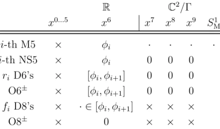
produces the so-called k-center Taub-NUT space, which gives rise tok D6-branes upon reduction to type IIA [53], together with N NS5-branes. The situation is summarized in table1.

Supersymmetry is halved due to the orbifold, and the (2,0) tensor multiplets from the M5’s each reduce to a (1,0) tensor multiplet plus a (1,0) hypermultiplet. We then have N ₋1 finite-length stacks each containing k D6-branes, giving rise to a chain of SU(k) gauge groups, as well as two semi-infinite D6 stacks.5 The N NS5’s contribute

NT =N−1 tensor multiplets as well asNT−1 =N−2 bifundamental hypermultiplets.

This is the type IIA description of this orbifold (1,0).

5_{In principle we would have U(}_k_{) gauge groups. The U(1) centers are all anomalous, but the}

(8)

R C2/Γ x0...5 x6 x7 x8 x9 S_M1

i-th M5 _× φi · · · ·

i-th NS5 _× φi 0 0 0

ri D6’s × [φi, φi+1] 0 0 0

O6± _× [φi, φi+1] 0 0 0

fi D8’s × · ∈[φi, φi+1] × × ×

O8± _× 0 _× _× _×

Table 1: NS5-D6(-O6)-D8(-O8) brane scan. A _· means the brane is sitting at a point along that direction;_×means it is infinitely extended along that noncompact direction. WhenΓ =Dk O6-planes

are present, and are overlaid onto the D6-branes. The O8-plane can either sit at 0, between the first NS5 atφ1 and its image at −φ1, or be stuck on the first NS5 say atφ1, which we choose to put at 0.

The real scalars φi inside the tensor multiplets are related to the positions of the

NS5’s along directionx6: We say we are on the tensor branch of the (1,0) SCFT when we give (nonzero) vevs to these scalars. This corresponds to having finite-coupling Yang– Mills terms in the Lagrangian of the quiver, and separates all NS5’s.6 In particular, we see from figure 1athat the left- and rightmost SU(k)’s are actually flavor groups, since they are associated with (two stacks of) semi-infinite D6-branes. Through a Hanany– Witten move we can trade each of the two for a stack of D8-branes sourcing a nonzero Romans mass F0 (although the latter has to vanish globally), where each D6 ends on

a different D8. The k D8’s contribute k fundamental hypermultiplets of the left- and rightmost gauge groups (see figure1b). We can now activate vevs for the former (much as in [54, 55]), and slide finite segments of D6-branes trapped between two D8’s off to infinity. We have modified the tail structure of the linear quiver by moving onto the Higgs branch of the SCFT.

In particular, its quiver will be characterized by two “massive tails” (of “lengths”

i = 1, . . . , L and N ₋ i = N ₋ 1, . . . , N ₋ R), where D8’s cross D6-branes, and a central “massless plateau” (of length N ₋L₋R) where there are no D8-branes and the Romans mass is identically zero. (Clearly, there can be nongeneric situations where the plateau disappears or we only have one massive region.) This engineers a situation (depicted in figure 1d) where we can have fi fundamental flavors of the i-th gauge

6_{The numbers}_N

Tof dynamical tensor multiplets andNT−1 of bifundamental hypermultiplets are

now explained. One tensor multiplet scalar, corresponding to the center-of-mass motion of the quiver alongx6_{, decouples from the dynamics. Supersymmetry tells us the whole multiplet is lost. Then, only}

(9)

group, for i ₆= 0, N. The ranks ri − 1 of the SU(ri) gauge groups need not equal k₋1 anymore (but max

1≤i≤N−1ri = k), due to the various Higgsings we have performed.

However, in the massless plateau ri =k fori=L, . . . , N−R: We will dub this number

“height” of the plateau. To all this data one can easily associate combinatorial objects, in the form of two Young tableaux ρL, ρR (one for each tail). They are associated to a

(ordered) partition of the maximal rank k (and therefore to a nilpotent orbit of su(k) [56]) as follows.7 Define the depth (ρt)i of the rows of the transposed tableau ρt by

(ρt)i :=ri −ri−1 =:si, i = 1, . . . , L (for ρL) or i = N −R, . . . , N −1 (for ρR). Then ρL = [ρ1, ρ2, . . . , ρl] and−ρR =−[ρ1, ρ2, . . . , ρr] are partitions of k:

l

X

i=1

(ρL)i = L

X

i=1

(ρt_L)i =rL=k=rN−R=− R

X

i=1

(ρt_R)N−i =− r

X

i=1

(ρR)N−i . (2.1)

(The numbers l, r depend on the specifics of the tableaux at hand, and can easily be found by transposingρt_L,R.) In the above equation we have crucially assumedr0 =rN =

0; this assumption will be relaxed momentarily. The theory at the origin of the Higgs branch – the “unHiggsed” theory in figure 1a– will be labeled by two trivial partitions

ρt_L = ₋ρt_R = [1,1, . . . ,1] =: [1k] (both corresponding to the trivial nilpotent orbit _{0_} of dimension zero), since ρL = −ρR = [k] = r1 = −(−rN−1). The Higgsed quiver of

figure 1chas instead

ρt_L= ρL= ; −ρtR = −ρR = (2.2)

corresponding to the nilpotent orbits_OL_[5,22_,1] and O_[6,4]R of su(10). Finally, gauge-anomaly cancellation implies [3]

fi = 2ri−ri+1−ri−1 =−(ri+1−ri) + (ri−ri−1) =−si+1+si >0 . (2.3)

The positivity of thefiimplies that the functioni7→ribe convex. A simple consequence

of this is that for i = 1, . . . , L the numbers ri have to grow, and to decrease for i = N ₋R, . . . , N.8 Given that the fi are the numbers of D8-branes sourcing a nonzero

Romans mass F0, the latter will be monotonous and decreasing along x6, crossing a

7_{See [}₃₂_{] for a full exploitation of this observation in the more general context of (1}_,_{0) quivers}

engineered through F-theory.

8_{The minus in front of}_ρ

Raccounts for the fact that in the right Young tableau the columns have

(10)

region where it is zero (the massless plateau) and eventually becoming negative (the right massive tail), so that we always have D8-branes instead of anti-D8’s.

As already mentioned, we can further generalize this situation by slightly modifying the quiver in figure 1d. In fact, as long as relation (2.3) is satisfied at each node, we can have nonzero numbers r0, rN of flavor D6-branes escaping off to infinity at the left

and right of the quiver. For i= 0, N the left hand side of (2.3) then reads r0+f1 and rN+fN−1respectively. The left, right Young tableau will give a partition ofkL :=rL−r0, kR :=rN−R−rN respectively, withk =rL=rN−Rthe height of the plateau. As we will

see, although we are simply adding some flavors of the first and last gauge groups, this has the effect of modifying the “poles” of the internal space of the dual supergravity AdS vacuum (topologically, anS3).

We now move on to describe how the AdS7 vacua of [30, 31, 27] are related to the

above constructions. A possible interpretation of these vacua as near-horizon limits of the brane configurations first appeared in [27]. (See also [57, 58, 59, 52, 60] for more general Ansatze of localized intersecting brane metrics with AdS7 near-horizon.)

Bringing all NS5’s on top of each other (the origin of the tensor branch, where the SCFT sits), we can imagine zooming in close to the NS5-D6 intersection, say at x6 = 0. This limit cannot forget the information about the D6-D8 intersection though, which labels the particular SCFT and is collected in the Young tableaux ρL,R of the linear

quiver. In fact, the D6-D8’s transform into magnetized D8 sources in the supergravity solution (with D6 charge smeared over their common worldvolume); the N NS5’s turn into N units of quantized H flux. Intuitively, two among directions x6 and x7,8,9 mix, and parameterize the base of the three-dimensional (compact) internal space M3 of

the AdS vacuum, plus its radial direction. In fact unbroken supersymmetry dictates that this space be a fibration S2 ,_→ M3 → I = [0, N], where the (finite-length) base

interval is now parameterized by a coordinate we callz. The remaining seven directions parameterize AdS7 and are filled by the D8 sources, which also “wrap” an S2 fiber

inside M3.9 Their position along z is fixed by supersymmetry [30, 1]. Moreover the

Romans mass F0 that is sourced by the branes will be a step function supported on I:

Its value decreases whenever we cross a D8 stack starting from z = 0.

The supergravity vacuum (metric, dilaton, warping factor, fluxes) can be defined in terms of a single cubic polynomial of z that we call α(z); it is defined piecewise in the subintervals [i, i+ 1] we decide to divide I into (i = 0, . . . , N ₋1). In the coordinate

9_{The D6 charge of the magnetized D8’s is equivalent to turning on a (nontrivial) gauge bundle on}

(11)

z, the position of the i-th D8 stack is conveniently fixed to be at z = i (i.e. the lower endpoint of [i, i+ 1]) by the second derivative ofα(z), namely ¨α(z)_|z=i =−(9π)2ri. The

number of D8’s in the i-th stack at z = i defines the value of the Romans mass F0 in

[i, i+ 1] (which is related to the third derivative of α(z) via (2.12) and (2.11), given below). This way, the supergravity vacuum depends on the quiver data only through

F0. The data associated with the tails of the quiver (i.e. the Young tableaux, when D8’s

are present, or simply the groups SU(f1), SU(fN−1) when we have semi-infinite flavor

D6’s) dictates what the coefficients of the polynomial α(z) are for i _∈ [0, L] (where

F0 >0) andi∈[N−R, N] (whereF0 <0). In particular, fori= 0, N, such coefficients

will be called “boundary data”, and can be related to what kind of brane sources are located in the vicinity of the “poles” ofM3 at the extrema z = 0, N of the base interval I.

We remark that, in case r0, rN 6= 0, the left impression in figure 1e will be slightly

modified (as depicted in the right one): The smooth poles of the internal spaceM3 will

now be singular points for the metric due to the presence of (flavor) D6-brane sources. The creases representing magnetized D8 sources will be displaced alongz so as to satisfy (2.3). The correspondence that we have just sketched will be made much more precise in section 2.

2.1.2 Alternating SO-USp groups: M5’s on _C2/Dk

In case N M5-branes probe the _C2/Dk singularity, there are two interesting effects. In

M-theory, the M5’s “fractionate” (i.e. we haveN = 2M half-M5-branes) [61]; in the IIA reduction, we have O6-planes on top of D6-branes (intuitively, the former “lift” to the extra generator ofDkwhich is not present inAk−1) suspended bewteen NS5-branes. The

NS5’s also fractionate, producing a sequence of alternating SO(2k) and USp(2(k₋4)) gauge groups [28].10 (See figure2afor the brane setup and2bfor the unHiggsed quiver.) They will contribute NT =N −1 = 2M −1 (1,0) tensor multiplets. The first gauge

group is engineered through an O6− projection on SU(k), the second through an O6+ one (the O6 charge changes sign whenever the plane crosses an NS5, an effect first discussed in [62] for O4’s). The rank of both gauge groups is always even, a fact that is related to the number of k mirror pairs of D6’s under the O6 projection. Moreover, the “jump” in the ranks of consecutive gauge groups (2k _→2k₋8 or 2k₋8_→2k) can

10_{For real compact symplectic groups we use the following notation: USp(2}_k_{) = Sp(}_k_{), of real}

(12)

be explained in field theory as a consequence of condition (2.3), and in string theory as the fact that an O6±-plane has _±4 D6 charge (thereby modifying the effective number of D6’s in a finite-length stack).

As before, we can modify the tail structure of the orbifold SCFT by adding D8-branes, as depicted in figure2c. Gauge-anomaly cancellation at each node enforces the following condition [32, Eqs. (4.11), (4.12)] (which can be derived from (3.10)):

fi+ 16 = 2pi−qi−qi−1 , gi−16 = 2qi−pi−pi−1 ; i= 1, . . . , M . (2.4)

fi (gi) is the number of half-hypermultiplets in the (real) vector representation of a

gauge SO(pi) (USp(qi)) group;N−1 = 2M−1 whenf1 =p1 = 0 (i.e. the quiver starts

off with a USp(q1) gauge group), or N −1 = 2M if f1, p1 6= 0.

As usual, adding D8-branes corresponds to a Higgsing of the theory which will be specified by two nilpotent orbits ofso(2k) (one for each tail), defined by two (transposed) “even” partitions λt of 2k [56, Thm. 5.1.4]. The quiver can now be written as in (the left frame of) figure 2d. (Notice that in a Higgsed quiver we might encounter odd-rank SO groups as well, see e.g. [48, Fig. 6]. This corresponds to a so-called O6f

−

, whereby a half-D6 is stuck on the O-plane. K-theory then requires having an odd quantum n0

of Romans mass F0 [63], i.e. an odd number of D8-branes crossing the D6-O6f

−

stack.) For each massive tail, suppose we define ρi := λti −λti+1 for i = 1, . . . , n−1 and ρn :=λtn using λt = [λt1, λt2, . . . , λtn]. (The number n can be found by transposing the

chosen partition.) The ρi give the numbers of D8-branes crossing the i-th D6-O6 stack,

whereas the “ranks” are defined as sums of parts of λt as follows [32, Eq. (4.34)]:

%i :=−8 + i

X

k=1

λt_k , for i odd ; %i := i

X

k=1

λt_k , for ieven . (2.5)

Here%i is the rank of a gauge USp (SO) group foriodd (even). In figure2d, the former

is represented by a black circle, the latter by a gray one. The number of D6-branes in each color stack is given by 2ri := Pi_k=1λtk, and this is what we will call rank of

the gauge group in the large N computation of sections 3.2 and 4.2. (The factor of 2 comes from counting physical branes and their images, in our conventions.) Using this partition-inspired notation, (2.4) reads (for each massive tail) [32, Eq. (4.36)]:

ρ2i−1+ 16 = 2%2i−1−%2i−2−%2i , ρ2i−16 = 2%2i−%2i−1−%2i+1 ; i= 1, . . . , n . (2.6)

(13)

quiver looks like that in figure 2b.

We also remark that, in the SO-USp case, the perturbative IIA picture may break down due to the appearance of (hypermultiplet) spinor representations which cannot be engineered in string theory. One must then turn to the F-theory description of the (1,0) theory [28, 48, 32]. However one may still use a “formal” massive IIA brane configuration (where we formally allow for a non-positive number of D6-branes in some finite-length stacks) to compute theaconformal anomaly of the (1,0) quiver engineered in F-theory [32]. As it turns out, the result agrees with the nonperturbative F-theory calculation. [32] also found a necessary and sufficient condition to engineer one such formal massive IIA quiver: The largest part λt₁ of an ordered transposed even partition

λt of 2k is less or equal to 8. One immediately notices that the principal (or regular) orbit _O[2k−1,1] of so(2k) satisfies this condition (since λt = [2,12k−2]). In section 5.1 we

will construct for the first time the AdS7 vacuum dual to this quiver (depicted in figure

5.1a), and we will extract its a conformal anomaly at largeN.

The corresponding supergravity vacua will differ from those dual to NS5-D6-D8-engineered quivers only for the presence of a nonzero constant term of the cubic polyno-mialα(z) in the intervals [0,1] and [N₋1, N]. We call themα0 (whenα(z) is supported

on [0,1]) andαN (whenα(z) is supported on [N−1, N]). These constants are vanishing

in the pure SU(k) case, but are nonvanishing when O6-planes of negative charge are present at the end of the quiver. As we will explain in greater detail in section 2.3,

α0, αN can indeed be related to the effective D6 charge of a D6-O6− source localized at

the poles of the internal spaceM3. This charge is given by ˜r0,N :=−4+2n2 =−4,−2,0,

withn2 = 0,1,2 pairs of D6-branes, or by ˜r0,N :=−4+2n2+21₂ =−3,−1 withn2 = 0,1

if also a half-D6 is present. (For n2 = 2 the total D6 charge is zero, and the pole is

regular.) A nonvanishing D6 charge n2 (or n2 +1₂) can then be associated with flavor

symmetries SO(g1,M = 2n2) (or SO(g1,M = 2n2+ 1)) of positive rank in the unHiggsed

quiver of figure 2bor the left Higgsed quiver of figure 2d(when f1 =p1 = 0).

In both cases, the metric will be singular at the poles, and the dilaton divergent. The S2 fibers of M3 will be replaced by RP2 ones due to the antipodal action of the

O6-planes.

2.1.3 SO or USp flavor, USp,SO,SU gauge groups: O8± onto D8’s

(14)

two consecutive NS5’s along x6 (i.e. an NS5 at φi >0 and its image at −φi) and when

the O8 is stuck at the location φi of an NS5.11 In the second case there exists only the

first possibility. Given that the O8-plane acts as a mirror along direction x6, we decide to put the origin ofx6 at its position. We will describe the linear quiver that ensues by considering only the “physical half” (say the one supported on [0,+_∞)) of the gauge and flavor groups.

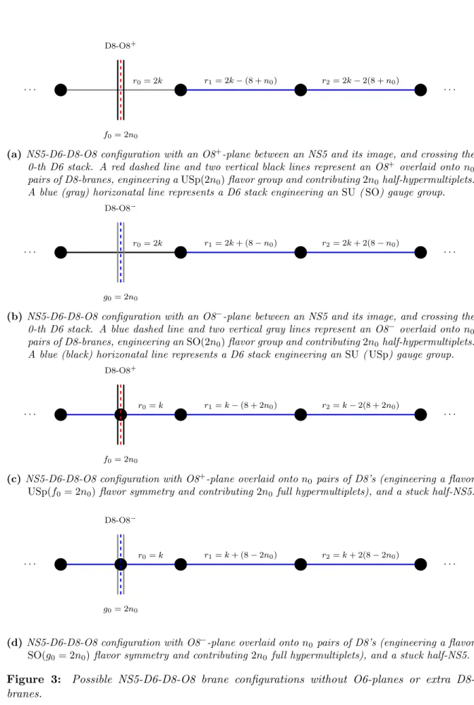
Let us first discuss the case without O6-planes. All consistent brane configurations are depicted in figure 3. In the first situation the O8±-plane (carrying _±16 units of D8 charge) will cross the (i = 0)-th segment of r0 = k D6-branes, projecting the gauge

group to SO(2k) or USp(2k) respectively.12 (The first NS5 at φ1 > 0 contributes a

single (1,0) tensor multiplet and a decoupled hypermultiplet which is neutral under the 0-th gauge group.) The next finite-length D6 stacks are not affected by the O8 projection, and their gauge group will be SU(ri) with even ranks ri = 2k∓i(8±n0) for i= 1, . . . , N₋1. As we will see, this is obtained by repeatedly applying condition (3.10) (which is a generalization of (2.3)) at each node, starting with r0 = 2k and f0 = 2n0

half-hypermultiplets (i.e. flv₀ = 1₂ in (3.10)). For i = N the semi-infinite D6-branes engineer an SU(rN = 2k∓N(8−n0)) flavor group.

We can now add more D8-branes (as in the pure SU(k) case), and engineer a left massive region, followed by a massless plateau, followed by a right massive region as long as condition (3.10) is satisfied. (Notice that, without extra D8’s, the number k

is constrained by N and n0 upon requiring 2k ∓N(8±n0) ≥ 0, in order to have a

meaningful SU(rN) flavor group). Moreover, the n0 D8 pairs overlaid onto the O8±

engineer an extra USp(2n0) (SO(2n0)) flavor symmetry. Finally, on top of the fN−1

fundamental (of SU(rN−1)) hypermultiplets contributed by D8-branes, we can have rN

flavor D6-branes escaping off to infinity. The quivers are depicted in figure 4a.

A very interesting subcase arises when k = 0 _⇒ r0 = 2k = 0, i.e. the first gauge

group is empty, and we stick say 8₋n0 D8 pairs on the O8− (see figure4c). There is no

orientifold projection on any of the gauge groups, and condition (2.3) simply imposes

ri = n0i for i = 1, . . . , N −1 (with a flavor symmetry SU(rN = N n0) on the right).

The (1,0) SCFT corresponding to this quiver is very similar to the so-called (rank-N) E-string theory [8], with the crucial difference that it cannot be engineered in M-theory

11_{Given that}_x6_{parameterizes}

R, we need not worry about D8 charge cancellation, but we still need to impose gauge-anomaly freedom, (3.10), i.e. an appropriately modified version of (2.3).

12_{Notice that, because of the projection around} _x6 _{= 0, the 0-th stack of D6-branes engineers a}

(15)

because of the D8’s (sourcing a nonzero Romans mass F0 = n_2π0). For this reason it was

dubbed (rank-N) “massive E-string theory” in [52]. (In particular whenn0 = 1 we have

an extraE8 flavor symmetry on the left, whose presence can be argued for by lifting the

particular D8-O8− system to M-theory as in [64];13 more generally, for 1_≤ n0 ≤ 8 we

have an E1+(8−n0) symmetry, using the definitions of [66].) The quiver was constructed in [52, Fig. 6] (which we reproduce in figure 4c), the dual AdS7 vacuum is given by [52,

Eq. (5.2)] and itsaconformal anomaly at largeN by [52, Eq. (5.13)].14 Given that this case has already been discussed at length in [52], in the remainder we will only treat the generic case where k₆= 0, i.e. r0 6= 0.

In the second situation, the O8± sits on top of a half-NS5-brane stuck on the plane, at x6 = 0. The orientifold projects out the tensor multiplet contributed by that NS5, does not act on the gauge group SU(r0), but acts on the bifundamental matter

com-ing from strcom-ings D60-image D60: We have a hypermultiplet in the (anti)symmetric of

SU(r0 =k). If we also overlay n0 pairs of image D8’s onto the O8±, all gauge groups

will be SU(ri = k∓i(8±2n0)) for i = 1, . . . , N −1, and we have a flavor symmetry

SU(rN =k∓N(8±2n0)) (again, this is due to (3.10)). We can also add D8-branes as

usual. The quivers are depicted in figure 4b.

The corresponding supergravity vacua will be defined in terms of a polynomialα(z) that, in the first subinterval z _∈[0,1], is characterized by a nonzero constant term α0

as well as coefficientr0 of the quadratic term, and in the last subinterval z ∈[N−1, N]

by a nonzero quadratic coefficient rN (this is a singular pole), but vanishing constant

term αN, as the right tail of the quiver is the same as for the pure SU(k) case. The

correspondence will be made more precise in section 2.

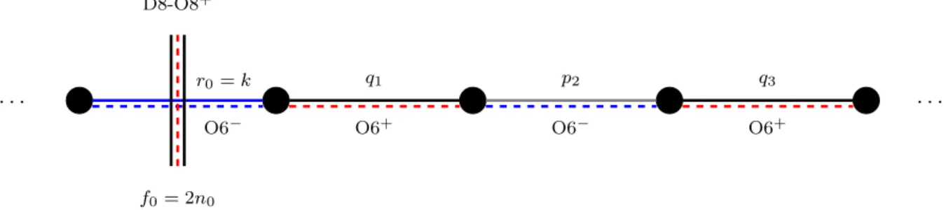
Let us now discuss the case with O6-planes overlaid onto D6-branes. The brane configurations are depicted in figure5. Given that the O6 charge changes sign whenever the former crosses an NS5, the situation where an O8 is stuck on the latter at x6 = 0, reflecting an O6± into itself, is not consistent. Thus we only need to consider the first situation (O8-plane between an NS5 at φ1 > 0 and its image at −φ1). The

combined O6+-O8− projection produces an SU(r0 = k) gauge group (i.e. only half of

the k D6 pairs under the O6 projection count), followed by a sequence of gauge groups

13_{The nonperturbative enhancement SO(2(8}

−n0))→E1+(8−n0)is due to D0-branes [65,66], which become tensionless asgs→ ∞sinceTD0∼g−s1.

14_{In that formula} _M _{is the number of D6-branes in the rightmost semi-infinite flavor stack, i.e.}

(16)

SO(pi)×USp(qi) for i = 1, . . . , N −1, and an SO(pN) or USp(qN) flavor symmetry,

according to the particular theory at hand (i.e. qN = 0 or pN = 0 respectively). Notice

that by simultaneously flipping the O6 and O8 charge we can exchange the gauge factors as to produce a sequence USp(qi)×SO(pi). Once again, we can add flavors of

each gauge group by inserting D8-branes across the finite-length D6 stacks (e.g. n0 D8

pairs overlaid onto the O8±-plane will produce a USp(2n0), respectively SO(2n0), flavor

group) as long as conditions (3.10) are satisfied at each node. The quivers are depicted in figure 5c.

The supergravity vacua will be characterized by a smooth pole of M3 at z = 0, i.e.

the cubic polynomial α(z) supported on [0,1] will have nonvanishing constant term α0

and quadratic coefficient r0 = k, and by a singular pole at z = N, that is the cubic

polynomial will have nonvanishing constant termαN but vanishing quadratic coefficient rN (due to the rightmost D6-O6− stack of total negative charge), or vanishing αN but

nonvanishing rN (due to the rightmost D6-O6± with total positive charge). The fibers

(17)

· · ·

f1=k r1=k rN−1=k fN−1=k

(a) The reduction to IIA of N M5’s probing C2/Ak−1. Circles represent NS5’s spread out along x6

(the horizontal direction); solid black lines represent finite-length D6-branes. r0 =rN = 0, given

that the 0-th andN-th stacks are made of (semi-infinite) flavor D6-branes.

f1=k |

•

r1=k−r2•=k− · · · − rN−•2=k −

fN−1=k |

•

rN−1=k

(b) The fully unHiggsed quiver engineered by the brane configuration in figure 1a. Blue circles rep-resent SU(ri) gauge nodes (vector multiplets, D6i-D6i strings), connected by bifundamental

hy-permultiplets (D6i-D6i+1 strings) and tensor multiplets (D6i-NS5i strings). Red boxes represent SU(fi)flavor nodes, connected to the former by fundamental hypermultiplets (flavor D6i - color

D6i strings). The f1, fN−1=k fundamental flavors of theSU(r1=k) andSU(rN−1 =k) gauge

groups respectively are equivalently engineered by k semi-infinite D6-branes or kD8-branes via a simple Hanany–Witten move (that does not modify the rest of the configuration).

· · ·

4 7 8 6 4 2

f1= 1 f2= 2 f13= 1

(c) Adding D8-branes to the setup in figure 1a, and Higgsing the theory as in [55]. Vertical lines (extending along directionsx7,8,9_{) represent flavor D8-branes crossing the D6-branes.}

1 |

•₄ −

2 |

•₇ −•₈ −•₉ −

1 |

•

10−10• −10• −10• −10• −10• −

1 |

•

10−•9−

1 |

•₈ −•₆ −•₄ −•₂

(d) A more general quiver corresponding to the brane setup of figure1c: N = 17,L= 5,R= 6, the partitions of10are given by (2.2), and r0=rN = 0. The SCFT is at a generic point of its tensor

and Higgs branch.

(e) The internal space M3 ∼=S3 of the AdS7 vacuum which is dual to the quiver in figure 1d. The

impression depicts the S2 _{fibers over the base interval} _I _{= [0}_{, N}_] _{parameterized by} _z _{(related to}

x6 _{by the near-horizon limit). Notice that the poles of} _S3_{, at the extrema of the base interval,}

are smooth points for the metric (the S2 _{fiber smoothly shrinks to zero size). A black crease}

represents a stack offi magnetized D8-branes (we will call stack even a single D8-brane) wrapping

a particularS2 _{fiber over the point} _z₌_i_.

(18)

1

2 12

· · ·

1

2 12

g1= 2k q1= 2k−8 qM = 2k−8 gM = 2k

O6− O6+ _O6+ _O6−

(a) The reduction to IIA ofM M5’s probing_C2_/D

k. A 1₂ superposed on a black dot indicates a

half-NS5-brane. A red dashed line represents an O6+ _{overlaid onto}_k_{pairs of D6-branes (the stack has}

an effective2(k₋4)D6 charge), a blue one an O6− overlaid onto k pairs.

g1=2k |

•

q1=2k−8−p1=2k• −q2=2k•−8− · · · −pM−•1=2k−

gM=2k

|

•

qM=2k−8

(b)The quiver engineered by the brane configuration in figure2a. Black (gray) circles representUSp(qi)

(SO(pi)) gauge groups, whereas black (gray) squares represent USp(fi) (SO(gi)) flavor groups.

There areM₋1 SO(2k)gauge groups andM USp(2(k₋4))gauge groups,NT=N−1 = 2M−1

tensor multiplets andN₋2 = 2M₋2 hypermultiplets (both represented by a₋).

1 2

· · ·

%1 %2 %3 %4

ρ1 ρ2 ρ3 ρ4

(c)Stacks ofρiD8-branes crossing the D6-O6 stacks in a massive tail. The O6±projects theSUflavor

group engineered by thei-th D8 stack toSO(ρi)(USp(ρi)), which is represented by a vertical gray

(black) line. All NS5’s are half-branes.

f1 |

•

p1 − g1

|

•

q1 − · · · −

fi

|

•

pi − gi

|

•

qi − · · · −

fM

|

•

pM − gM

|

•

qM

∼

=

ρ1 |

•

%1−

ρ2 |

•

%2− ρ3

|

•

%3 −

ρ4 |

•

%4 − · · ·

(d) A more general quiver corresponding to the brane setup of figure 2c. On the left we use the same convention as in figure 2b (there are N = 2M or 2M ₋1 gauge groups, the latter when

p1=f1= 0); on the right we use the partition-inspired convention (2.5),(2.6).

(19)

· · · r0= 2k r1= 2k−(8 +n0) r2= 2k−2(8 +n0) · · ·

f0= 2n0 D8-O8+

(a) NS5-D6-D8-O8 configuration with an O8+_{-plane between an NS5 and its image, and crossing the}

0-th D6 stack. A red dashed line and two vertical black lines represent an O8+ _{overlaid onto}_n 0

pairs of D8-branes, engineering aUSp(2n0)flavor group and contributing2n0half-hypermultiplets.

A blue (gray) horizonatal line represents a D6 stack engineering anSU(SO) gauge group.

· · · r0= 2k r1= 2k+ (8−n0) r2= 2k+ 2(8−n0) · · ·

g0= 2n0 D8-O8−

(b) NS5-D6-D8-O8 configuration with an O8−-plane between an NS5 and its image, and crossing the 0-th D6 stack. A blue dashed line and two vertical gray lines represent an O8− overlaid onton0

pairs of D8-branes, engineering anSO(2n0)flavor group and contributing2n0half-hypermultiplets.

A blue (black) horizonatal line represents a D6 stack engineering anSU(USp) gauge group.

· · · r0=k r1=k−(8 + 2n0) r2=k−2(8 + 2n0) · · ·

f0= 2n0 D8-O8+

(c) NS5-D6-D8-O8 configuration with O8+_{-plane overlaid onto}_n

0 pairs of D8’s (engineering a flavor

USp(f0= 2n0)flavor symmetry and contributing2n0 full hypermultiplets), and a stuck half-NS5.

· · · r0=k r1=k+ (8−2n0) r2=k+ 2(8−2n0) · · ·

g0= 2n0 D8-O8−

(d)NS5-D6-D8-O8 configuration with O8−-plane overlaid onton0 pairs of D8’s (engineering a flavor

SO(g0= 2n0)flavor symmetry and contributing2n0 full hypermultiplets), and a stuck half-NS5.

(20)

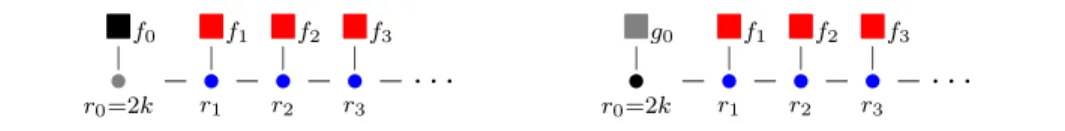
f0 |

•

r0=2k−

f1 |

•

r1 −

f2 |

•

r2 −

f3 |

•

r3 − · · ·

g0 |

•

r0=2k−

f1 |

•

r1 −

f2 |

•

r2 −

f3 |

•

r3 − · · ·

(a) The left quiver corresponds to the brane setup of figure3a (O8+ between NS5 and its image), the right one to that of figure3b(O8− _{between NS5 and its image).}

f0 |

•

r0=k−

f1 |

•

r1 −

f2 |

•

r2 −

f3 |

•

r3 − · · ·

g0 |

•

r0=k−

f1 |

•

r1 −

f2 |

•

r2 −

f3 |

•

r3 − · · ·

(b) The left quiver corresponds to the brane setup of figure 3c(O8+ stuck on a half-NS5); there is a hypermultiplet in the symmetric representation ofSU(r0=k), which we represent by. The right

one to that of figure3d(O8− _{stuck on a half-NS5); there is a hypermultiplet in the antisymmetric}

representation ofSU(r0=k), which we represent by .

· · · r0= 0 r1=n0 r2= 2n0 · · · fN−1=N n0

g0= 2(8−n0) D8-O8−

(c)NS5-D6-D8-O8− brane configuration engineering a rank-N massiveE1+(8−n0)-string theory on the

tensor branch (simply called massive E-string theory when n0 = 1). There are 8−n0 pairs of

D8-branes overlaind onto the O8−. The flavor group SO(2(8₋n0))can be argued to enhance to

E1+(8−n0) at strong coupling [66].

g0=2(8−n0) |

•

r0=0−r1=n• 0 −r2=2n• 0−r3=3n• 0− · · · −

fN−1=N n0 |

•

rN−1=(N−1)n0

(d) The rank-N massive E1+(8−n0)-string theory quiver. The first gauge group is empty, but there is

a tensor multiplet (withE1+(8−n0) enhanced flavor symmetry) which we represent by the leftmost

−.

Figure 4: Quivers engineered by NS5-D6-D8-O8± brane configurations. Notice that we have added possible flavors for each gauge node for i= 1, . . . , N₋1. (f0=g0 = 2n0 is the rank of the leftmost flavorUSp/SO group respectively.) This can be done as long as condition (3.10)

(21)

· · · r0=k · · ·

q1 p2 q3

O6− _O6+ _O6− _O6+

f0= 2n0

D8-O8+

(a)NS5-D6-O6-D8-O8 configuration with O8+_{-plane between an NS5 and its image, and crossing the}

0-th D6-O6− stack. A red vertical dashed line paired up with two black lines represent an O8+

overlaid onto n0 pairs of D8-branes, engineering a USp(2n0) flavor symmetry and contributing

2n0 half-hypermultiplets. A blue (black/gray) horizonatal line represents a D6 stack engineering

anSU(USp/SO) gauge group.

· · · r0=k · · ·

p1 q2 p3

O6+ _O6− _O6+ _O6−

g0= 2n0

D8-O8−

(b)NS5-D6-O6-D8-O8 configuration with O8−-plane between an NS5 and its image, and crossing the 0-th D6-O6+ stack. A blue vertical dashed line paired up with two black lines represent an O8− overlaid onto n0 pairs of D8-branes, engineering an SO(2n0) flavor symmetry and contributing

2n0 half-hypermultiplets. A blue (gray/black) horizonatal line represents a D6 stack engineering

anSU(SO/USp) gauge group.

f0 |

•

r0=k− g1

|

•

q1 −

f2 |

•

p2 − g3

|

•

q3 − · · ·

g0 |

•

r0=k−

f1 |

•

p1 − g2

|

•

q2 −

f3 |

•

p3− · · ·

(c) The left quiver corresponds to the brane setup of figure 5a (O8+_-O6− _{combined projection), the}

right one to that of figure5b(O8−-O6+ _{combined projection). Notice that we have added possible}

flavors for each gauge node. This can be done as long as conditions (3.10) are satisfied. Notice the difference with figure 2d(we use same colors and names for gauge and flavor nodes).

(22)

2.1.4 The holographic limit

Having heuristically explained how the near-horizon limit of the various brane configu-rations might work, we now set out to find the correct “holographic limit”. By this we mean the limit that suppress curvature andgs corrections to the closed string spectrum

sourced by the brane setup, allowing us to reliably use the classical AdS7 supergravity

vacua. Usually this also turns out to be a so-called largeN limit in the dual field theory. For the NS5-D6(-O6)-D8(-O8) configurations that engineer six-dimensional (1,0) linear quivers, [1] identified the correct limit to achieve the aforementioned suppression and at the same time keep track of the nontrivial information contained in the Young tableauxρL,R. (We know that this information labels the Higgsed theory and is

associ-ated with the massive tails of the quiver, so it should not be washed away in the limit.) The limit is the following:

N, L, R, k, ri → ∞ , L N,

R N,

k N,

ri

N finite. (2.7)

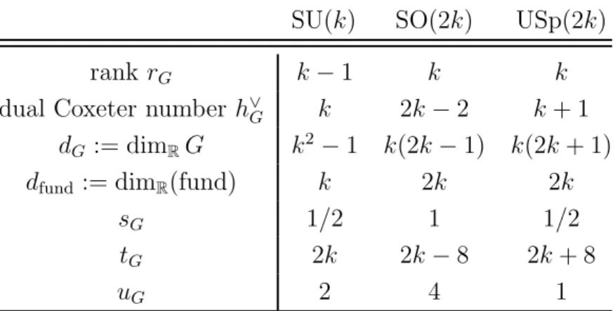
In particular we see that, in six dimensions, “large N” means infinite number of gauge groups. k, ri → ∞ also tells us that the ranks of the various gauge and flavor groups

are infinite. In light of table 3 this means that their dual Coxeter numbers (which will play an important role in the holographic match of a) are infinite, and approximate the ranks: h∨_G _∼ rkG _{→ ∞}. We will write _∼ to indicate the holographic limit of all relevant quantities.

2.2 Constructing generic solutions with

z

We shall now describe in greater detail how to construct the supergravity AdS7 vacua

dual to the quivers just introduced, by relying on the same combinatorial data.15

The generic AdS7 supergravity vacuum of massive type IIA can be described in

terms of a single function α(z) on which all physical fields (metric, dilaton, warping factor, fluxes) depend. The coordinatez parameterizes the base intervalI of the three-dimensional internal space M3, which is a fibration of two-spheres over I. The total

space of the fibration can be made compact by requiring that the fiber shrink at the extrema ofI. (Thus, topologically,M3 ∼=S3.) This in turn imposes boundary conditions

for the internal metric at the poles of S3. Different boundary conditions correspond

15_{Notice that, once we construct a general AdS}

7 vacuum of massive IIA, we can easily obtain AdS5

and AdS4ones from it by applying the one-to-correspondences in [67,68]. It is also possible to construct

(23)

to different physical sources, such as branes and orientifolds. The existence of these global solutions was first established numerically in [30].16 The solutions were later given a fully-analytic expression in [67], where the functionα(z) we just introduced was called β(y). Here, we will present the solutions as in [1], which further generalizes the formalism of [67].17

In [1] it was imposed that at the poles of S3 the metric be either regular or have the asymptotics corresponding to D6-brane sources. Under the correspondence between NS5-D6(-O6)-D8(-O8) brane configurations and AdS7 vacua we explained in the

pre-vious section, a regular asymptotics corresponds to having a stack of D8-branes (with D6 charge smeared on the common worldvolume) wrap an S2 fiber in the vicinity of the pole, whereas the second case to a stack of D6-branes localized at the pole. Both D6 and D8 sources are spacetime filling. (These statements are to be understood after having taken the near-horizon limit of the localized closed string spectrum – sourced by the brane configuration – which produces the AdS vacuum.)

In this work we generalize this situation, and allow for several new boundary con-ditions. For instance, we will construct the most general solution with D6-brane poles and an O8-D8 wall along the equator of S3. A version of this solution – dual to the so-called massive E-string theory – has already appeared in [52]; here we will generalize it further. We will also see how to introduce O6-planes on top of D6-branes, and show what the boundary conditions for such a combined object look like.

Explicitly, the ten-dimensional metric reads

1

π√2ds

2 10 = 8

r −α

¨

αds 2 AdS7 +

r −α¨

α

dz2 + α

2

˙

α2₋₂_α_α_¨ds 2 S2

, (2.8)

whereas the dilaton

eφ(z) = 25/4π5/234 (−α/α¨)

3/4

√

˙

α2₋₂_α_α_¨ . (2.9)

(Morever, as reviewed in appendix A, ¨α <0.) We also have

B =π

−z+ αα˙ ˙

α2₋₂_α_α_¨

volS2 , F₂ =

¨

α

162π2 +

πF0αα˙

˙

α2₋₂_α_α_¨

volS2 . (2.10)

The (continuous) coordinate z parameterizes the base interval I = [0, N], which will

16_{See [}₇₀_,₇₁_{] for an earlier AdS}

7×S3Ansatz with smeared sources, and [72] for a local construction. 17_{A change of variables is needed to go from the presentation of [}₆₇_{] to that of [}₁_{] and the present}

(24)

be divided into subintervals [i, i+ 1], i = 0, . . . , N ₋1. The integer N is precisely the number of NS5-branes in the IIA configuration (and is related to the quantized flux of H via N = ₋_4π12

R

M3H, see e.g. [67, Eq. (5.42)]). The Romans mass F0 is a step function with different values for different subintervals [i, i+ 1], namely

F0 ={F0,1, . . . , F0,N} , F0,i+1 = 2πn0,i+1 = 2πsi+1 := 2π(ri+1−ri) , (2.11)

where n0,i∈ Z (due to flux quantization) and ri−1 are the ranks of the gauge groups

SU(ri) in a linear quiver description of the dual SCFT’s (in the pure SU case). The

above combinatorial relation between Romans mass and ranks was derived in [1, Eq. (2.15)]

As discovered in [67], the supergravity equations that each vacuum is a solution to reduce to a single ODE, which in the language of the present paper can be recast in the following form:18

...

α(z) =₋(9π)2si+1 , z ∈[i, i+ 1] . (2.12)

This allows us to determine α as well as its first and second derivative (which will be very useful in the following) by successive integration. Calling

y(z) :=₋ 1

18πα˙(z), q(z) :=

1

9πy˙(z) = −

1

2(9π)2α¨(z)≥0 , (2.13)

in each of the intervals z _∈[i, i+ 1] we have

α(z) =αi−2(9π)yi(z−i)−

(9π)2

2 ri(z−i)

2

− (9π)

2

6 si+1(z−i)

3 _, _(2.14a)

y(z) =yi+

9π

2 ri(z−i) + 9π

4 si+1(z−i)

2 _, _(2.14b)

q(z) = 1 2ri+

1

2si+1(z−i), (2.14c)

where y_i, α_i are integration constants. To determine the latter it suffices to impose continuity of α(z), y(z) at every interval upper endpoint z =i+ 1, for i= 0, . . . , L₋1 and then N₋R, . . . , N₋2. The results depend on the “boundary data” y0, yN, α0, αN

(which will be determined shortly) and the physical ranks ri, and read

2 9πyi =

2 9πy0+

1

2(r0+ri) +

i−1

X

k=1

rk , (2.15a)

(25)

and

αi =α0−(9π)(2i)y0−

(9π)2

6 ((3i−1)r0+ri)−(9π)

2 i−1

X

k=1

(i₋k)rk (2.15b)

for i_∈[1, L] and

2

9πyN−i =

2 9πyN −

1

2(rN +rN−i)−

i−1

X

k=1

rN−k , (2.15c)

αN−i =αN + (9π)(2i)yN −

(9π)2

6 ((3i−1)rN +rN−i)−(9π)

2 i−1

X

k=1

(i₋k)rN−k (2.15d)

for i_∈[1, R]. (The derivation is carried out in appendix B.)

We now have to determine the boundary data themselves. This can be done by imposing continuity atz =Landz =N₋R, which in turn implies the useful constraints [1, Eq. (2.20) and above (A.5)]:19

yN−R−yL=

9π

2 k(N −R−L) ,

αN−R−αL=

2

k(y 2

L−yN2−R) ;

⇔ yN−R−yL=

9π

2 k(N −R−L) ,

αN−R−αL=−9π(N −R−L)(yL+yN−R),

(2.16)

where rL = rN−R = k is the height of the massless plateau, which is equivalent to

maximum rank in each of the two massive regions. (2.16) are two equations, and in general cannot determine four independent parameters (y0, yN, α0, αN). However in all

practical situations we will encounter we only need to determine a subset of them, as some may be identically vanishing. This is because different brane or orientifold sources impose different boundary conditions on the internal part of the metric (2.8), telling us which boundary data are vanishing, and which are not.

A remark is in order here. In presence of O6-planes, finite-length D6 stacks will actually comprise ri → 2ri branes (i.e. we count both the physical ones and their

images) due to the orientifold projection, and the height of the plateau (the maximum rank) becomes k _→ 2k (see the discussion in section 2.1.2). (Moreover an SO gauge group engineered can have odd rank if there is a stuck half-D6 on top of the O6−, in which case the latter is known as O6f

−

.)

19_{Notice that there is a typo on the right-hand side of [}₁_{, Eq. (2.20)]:} 9π

4 should be replaced by 9π

(26)

2.3 Boundary conditions

Let us describe the possible boundary conditions of the internal metric around z = 0. (Those around z = N can be found analogously.) Let us define the quantity σ(z) :=

˙

α(z)2₋2α(z) ¨α(z) for convenience. Given (2.14), at the lower endpoint of each subin-terval [i, i+ 1] we have:

α(z)_|z=i =αi , α˙(z)|z=i =−2(9π)yi , α¨(z)|z=i =−(9π)2ri , (2.17)

and

σ(z)_|z=i =:σi = 2(9π)2(riαi+ 2y2i) . (2.18)

In terms of α(z), σ(z) the metric of the internal space M₃ reads (see (2.8)):

1

π√2ds

2 M3 =

−α_α¨(₍z_z)₎

1/2

dz2+R2(z)ds2_S2 , R2(z) :=

−α_α¨(₍z_z)₎

1/2

α(z)2

σ(z) . (2.19)

R2(z) is the squared radius of the S2 fiber over the generic pointz _∈[0, N]. To have a compact M₃ we should impose R2(0) =R2(N) = 0. Focusing on the first condition we see that this is equivalent to requiring

R2(0) = r

1/2 0 α

3/2 0

18π(α₀r₀+ 2y2 0)

= 0 _⇔ r0 = 0∪α0 = 0 . (2.20)

Moreover, recalling (2.9), the boundary value of the dilaton is found to be

eφ(0) = 23/4π437 α

3/4 0

r3/4₀ (r0α0+ 2y02)1/2

. (2.21)

The criteria of [52, Sec. 5.1] to determine which kind of physical object we have at the endpoint z = 0 can now be phrased as follows:

• regular pole (the metric is finite and the space approximates _R3): α₀ = r₀ = 0,

σ₀ ₆= 0 _⇒ y₀ ₆= 0. These are the boundary conditions considered in [1], and correspond to having magnetized D8-branes wrapping an S2 fiber close to the pole;

• D6 pole: α0 = 0, r0 6= 0, σ0 6= 0 ⇒ y0 6= 0. We will call D6 pole even one

(27)

• O6 pole: α0 ∝ r˜0 6= 0, r0 = 0, σ0 6= 0⇒ y0 6= 0. Also in this case the S2 fiber is

replaced by _RP2. The total D6 charge ˜r0 of the D6-O6− source is negative;

• O8 pole without D6 charge: r0 =σ0 = 0 ⇒y0 = 0. In this case φ(z), R2(z)→ ∞

as z _→ 0, as is appropriate for a D8-O8 source of divergent dilaton type.20 (α0

may not be zero, for otherwise R2(z) tends to a constant as z _→ 0.) These boundary conditions are appropriate for the AdS7 vacuum constructed in [52, Eq.

(5.2)], dual to the massive E-string theory (described in section 2.1.3). Therefore we will neglect this case in the following;

• O8-D8 pole with D6 charge: r0 6= 0, y0 = 0 ⇒ σ0 = 2(9π)2r0α0 (and as before α0 6= 0). In this case φ(z), R2(z) are finite and nonvanishing at z = 0, which

corresponds to the equator of M3 ∼=S3. (As already explained, the physical half

of the internal space lies in [0, N].) In other words, the D6-brane charger0resolves

the dilaton and metric singularity at z = 0. (For r0 →0 this case reduces to the

previous one.)

One can indeed check [30] that the metric ds2_M₃, dilaton, and the relevant bulk fluxes close to z = 0 have the correct asymptotics to justify the presence of the above brane and orientifold sources. We summarize all possible requirements in table 2.21 We now realize that there exist only two cases with a nonvanishing subset of boundary data:

• if regular or D6 poles occur atz = 0 andz =N then α0 =αN = 0 automatically,

and we simply need to determine y0, yN. These are two parameters, and can be

determined by (2.16). The result is given in (B.24) (plugging in α0 = αN = 0).

If O6 poles occur instead, α0 and αN do not vanish but can be determined via

an independent physical argument (namely by expanding the bulk F2 flux in the

vicinity of z = 0, N, respectively)22 which suggests the definitions

α₀ := 9 2π

˜

r0y0 r1

, α_N :=₋ 9 2π

˜

rNyN rN−1

, (2.22)

where ˜r0,r˜N =−4, . . . ,−1 can be interpreted as the effective D6 charge of a flavor

D6-O6− stack.23 Once again we can use (2.16) to determine y0, yN. The result is

given in (B.32).

20_{See [}₂₀_{] for another well-known example.}

21_{The analysis of the boundary conditions at the other endpoint,}_z₌_N_{, is greatly simplified if one}

labels the subintervals starting from the latter rather than z = 0, i.e. z _∈ [N₋(i+ 1), N₋i] with

i= 0, . . . , R₋1.

22_{This is shown in section}_B.3_. 23_{Notice that}_α

(28)

• The second case corresponds to having an O8 pole atz = 0. (The orientifold acts as a wall around the origin of the z direction, and we choose to parameterize the physical half of the space by z _∈[0, N].) In this case y0 = 0, hence we only need

to determine α0, yN, αN. Moreover αN either vanishes (in case of a regular or D6

pole at z = N) or can be defined as in (2.22) in terms of yN and the effective

charge of a D6-O6− stack, if the latter is present. We can then use (2.16) to find expressions for α0 and yN, which are given in (B.40) and (B.38) respectively.

asymptotics of ds2_M₃ at z = 0, N resp. α0,N y0,N r0,N

regular point: D8-branes ( ˙α2₋2αα¨₆= 0) 0 ₆= 0 0 D6 pole ( ˙α2₋2αα¨₆= 0) 0 ₆= 0 >0 O6 pole ( ˙α2₋2αα¨₆= 0) >0 ₆= 0 0 O8 pole with D6 charge at z = 0: ˙α2₋2αα¨_∝r₀α₀ ₆= 0 0 ₆= 0

Table 2: The requirements for having a regular point, a D6 or D6-O6± source, a D8-O8 source with (smeared) D6 charge at the poles of the supergravity solution, characterized by an internal space

S2 _,

→M3 → I = [0, N] (or RP2 ,→ M3 → I = [0, N]). Different sources impose different boundary

conditions on the metric of M3 at the extrema of the base interval I. Notice that we can have an

O8-plane only atz= 0. The former acts as a mirror along directionz, and we choose to parameterize the physical half of the space by z_∈[0, N].

3 Computation of

a

in field theory

After having explained how to engineer (1,0) theories with massive IIA AdS7 duals,

we now explain how to extract a very important observable of the SCFT, namely its a

conformal anomaly. We will then take the holographic limit of the latter, and compare it to the result obtained in supergravity.

The (eight-form) anomaly polynomial_I of a six-dimensional (1,0) SCFT is a sum of various contributions (see [51] and appendixD), which can be summarized as follows:24

I =α c₂(R)2+β c₂(R)p₁(T) +γ p₁(T)2+δ p₂(T) +_I_flavor . (3.1)

withα(z) in [0,1] given by (2.14a) withi= 0, the constant term is found to be proportional to

q

r2 1 ˜ r0y0, which requires ˜r0y0 > 0. Given that ˜r0 <0, we must also have y0 < 0. At large k, N, this can be

proven by directly inspecting (C.30a) (sinceP

iri >Pi i

Nri). A similar argument holds forαN. 24_c

(29)

The coefficients α, . . . , δ are functions of the group theory data, the number of tensor multipletsNT =N−1,25 and the so-called Dirac pairing defined in (D.17), namely the

matrix

ηij =nδij −δi i−1−δi i+1 , n={n0, . . . , nNT}. (3.2) Explicitly, they are given by:

α= 1

24(NT−NV) + 1 2(η

−1₎ ijh∨Gih

∨

Gj , (3.3a)

β = 1

48(NT−NV) + 1 12(η

−1₎

ijKih∨Gj , (3.3b)

γ = 1

5760(23NT−7NV+ 7NH) + 1 288(η

−1₎

ijKiKj , (3.3c) δ= 1

5760(−116NT+ 4NV−4NH) , (3.3d)

where NV and NH are the total numbers of vector and hypermultiplets respectively,

NV = NT

X

i=1

dGi , (3.4)

NH = NT

X

i=1

idi+flvi fidi+i i+1didi+1

, (3.5)

and

Ki :=h∨Gi−i Ind(ρi)−sGi i i−1di−1+i i+1di+1+

flv i fi

. (3.6)

h∨_G_i is the dual Coxeter number of the i-th gauge group Gi, sGi the constant defined in table 3, and the coefficients i, i i+1, flvi = {1,12,0} account for the presence of full

hypermultiplets (1) as appropriate for SU quivers, half-hypermultiplets (1₂) as appro-priate for alternating SO-USp quivers, or no hypermultiplets at all (0). Ind(ρi) is the

index of the hypermultiplet representation ρi of real dimensiondi := dimR(ρi).26 (The dimension is calledfi for flavor hypermultiplets.)

Finally, the a conformal anomaly is given by the following combination of anomaly

25_{In the F-theory construction of these (1}_,_{0) theories,}_N

T=N−1 coincides with the number of−2

curves in the base (after having blown down all possible₋1 curves).

26_{By index we mean the eigenvalue of the quadratic Casimir in the representation, normalized}

such as to be an integer. If ρ is an irreducible representation of the Lie algebra g associated with

G, then Trρ(TaTb) = Indρ δab. More intrinsically, it can be defined in terms of d := dimRρ and

(30)

polynomial coefficients [74, Eq. (1.6)]:

a= 384

7 (α−β+γ) + 144

7 δ . (3.7)

Plugging the expressions (3.3) into the above equation we obtain the very general for-mula (in which a sum over repeated indices is understood):

a= 1

210(199NT−251NV+ 11NH) +

+ 16 7

12(η−1)ijh∨Gih

∨

Gj −2(η

−1₎

ijKih∨Gj + 1 12(η

−1₎ ijKiKj

. (3.8)

In this section we shall compute explicitly the leading term of theaconformal anomaly in field theory for a few linear quivers as h∨_G_i _∼N _{→ ∞}, which we claim to be

a_∼ 192

7 (η

−1₎ ijh∨Gih

∨

Gj . (3.9)

This leading behavior can be proven by showing that the last two terms in parentheses in (3.8) are subdominant w.r.t. the first, namely (3.9). This is easily done as follows.

First of all, as explained above (D.14), the cancellation of the gauge anomaly in-volving the term ₁₆1 Tr(F_i4) implies the constraint

tGi =iαρi + i i−1di−1+i i+1di+1+

flv

i fi , (3.10)

where the constants tGi have been defined in (D.11),

tr_adj(F_i4) =t_G_itr_fund(F_i4) +. . . , (3.11)

andαρi is the quartic Casimir ofGi in the representationρi, which is defined in (D.12). (Notice that in the pure SU(k) case (3.10) precisely reduces to (2.3).)

As one can see from tables 3and 4by direct inspection, the above constants satisfy the following relations for h∨_G_i _∼N _{→ ∞}:

tGi ∼

h∨_G_i sGi

, αρi ∼ Indρi

sGi

. (3.12)

Using (3.10) inside (3.6), and subsequently plugging in (3.12), we immediately realize that Ki is independent of N (i.e. it tends to a constant as N → ∞), hence any term in

(3.8) with a bilinear involving Ki is subdominant w.r.t. (η−1)ijh∨Gih

(31)

We now turn to the computation of a in some important classes of theories. By specializing the general formulae provided below, one can easily obtain the leading contribution to the a anomaly of any (1,0) linear quiver with massive type IIA dual (including the so-called “formal” quivers of [32]).

3.1 SU quivers on the tensor branch

The possible brane configurations realizing linear quivers with only SU(ri) groups are

depicted in figures 1a (without D8-branes) and 1c (with D8-branes – the latter is a specific example, easily generalizable to others). In the first, we have semi-infinite flavor D6’s extending beyond the left- and rightmost NS5-branes; in the second, stacks of magnetized D8-branes. As explained in section 2.1.1, in the supergravity AdS7

solution we then have D6 (r0, rN 6= 0) or regular (r0 =rN = 0) poles respectively (see

table 2);α0 =αN = 0 in both cases.

The regular poles case has already been treated in [1]. Those results carry through to the case with D6 poles, i.e. the computation of a is totally equivalent in both cases. The ultimate reason is thatr0, rN only appear in the gravity computation as coefficients

of subleading terms (w.r.t. the dominant _O(N5) order), and are also washed away in the field theory computation asri ∼k, N → ∞. Thus we may completely neglect them.

The quivers, depicted in figures 1band1d, are given by a collection of SU(ri) gauge

groups (flavor groups for i= 0, N); therefore h∨_G_i =ri for i= 1, . . . , N −1 =NT. The

(inverse) Dirac pairing (D.23b) is the (inverse) Cartan matrix ofAN−1. Therefore:

a _∼ 192

7 (η

−1

D6)ijrirj . (3.13)

Dividing the sum over i, j into left massive region, massless plateau, and right massive region, and keeping only the leading terms in N, we find:

a_∼ 192

7

L

X

i=1

+

N−R−1

X

i=L+1

+

N−1

X

i=N−R

! _L X

j=1

+

N−R−1

X

j=L+1

+

N−1

X

j=N−R

!

(η_D6−1)ijrirj (3.14a)

7 192a∼

k2 N

1

12(N −L−R)

2₍_N2_{+ 2(}_L₊_R₎_N

−3(L₋R)2) +

+ k

N(N−L−R) (N −L+R) L

X

i=1

iri+ (N +L−R) R

X

i=1 irN−i

!

1712.03235.pdf

AdS

/CFT

with orientifolds

Contents

1

Introduction

2

Brane configurations in massive IIA and

super-gravity solutions

2.1

The dictionary between branes, quivers, and vacua

2.2

Constructing generic solutions with

z

2.3

Boundary conditions

3

Computation of

a

in field theory

3.1

SU quivers on the tensor branch