QUANTUM DYNAMICS OF EXCITED ELECTRONS FROM FIRST PRINCIPLES: HOT CARRIER RELAXATION AND ELECTRONIC STOPPING
Kyle G. Reeves
A dissertation submitted to the faculty at the University of North Carolina at Chapel Hill in partial fulfillment of the requirements for the degree of Doctor of Philosophy in the
Department of Chemistry.
Chapel Hill 2016
ABSTRACT
Kyle G. Reeves: Quantum Dynamics of Excited Electrons from First Principles: Hot Carrier Relaxation and Electronic Stopping
(Under the direction of Yosuke Kanai)
An understanding of dynamical properties of matter is often essential to developing a deeper understanding of systems and their behavior. Many important examples of complex electron dynamics are a result of excited systems such as in the photoexcitation of photosynthetic complexes or hot carrier relaxation in photovoltaic devices. Applying first-principles computational methods to describe these systems and their dynamics would be a valuable tool to gain a deeper understanding of the relationship between atomic structure and the non-equilibrium electron dynamics. Approaches based on the Born-Oppenheimer adiabatic approximation fail, however, as the separation of electron and nuclear motion is no longer valid in the presence of excited electrons. First-principles simulations that incorporate non-adiabatic effects represent an approach to properly simulating the quantum dynamics of excited electrons while maintaining predictive power.
For my parents Pamela and Brian, my brother Christopher,
AKNOWLEDGEMENTS
I would first like to thank my advisor Professor Yosuke Kanai for his attention and commitment to supporting me to develop as both a scientist and as an individual. From my first year as the only graduate student in his lab up until the very end, I am grateful for his consistent support and insight. I would like to thank him for giving me space to explore and allowing for opportunities to make mistakes. I am excited to continue our conversations on science and philosophy into the distant future. I would also like to thank Professor André Schleife for mentoring me during my first summer in the program. As I have begun to learn of the challenges and frustrations of being a research scientist, I regularly find myself thinking of his positivity and enthusiasm. I have also been incredibly fortunate to have been mentored by Professor Dhandapani Venkataraman from the University of Massachusetts-Amherst. His deep and genuine thirst to experiment and to share that excitement with the world was what drew me to chemistry, and it is what continues to inspire me.
To those members of the Kanai Group throughout my time at UNC, I am extremely grateful for your making such an endeavor possible. From the satirical use of our group’s unofficial motto “try to be normal,” it was clear to me that it was perfectly acceptable to come to work as fully and authentically myself. I would especially like to thank Lesheng Li, Yao Yi, Dillon Yost and Zoe Watson for their close friendship.
May our paths cross regularly. Micah Brown—I am forever grateful and deeply thankful for your support and the adventures throughout the last few years.
Thank you to the many individuals who I have come to know and who happen to not be chemists or physicists (yet). Damon Seils, Dr. Allison De Marco, Dr. Molly De Marco, Dr. Jeff Herrick, Michelle Johnson, Scott McRae, Dr. Jonathan Reside, Taylor Livingston, Professor Anthony Bale, Rev. Heather Concannon, Lydia Enriquez, Gale Stafford, Shannon Stockwell, Anne Dufault, Kara Jacobacci, Dr. Olivia Holston, Dr. Cindy Hopf, Dr. Joe Malatos, Nick D’Eramo, Maddie Hayes, Rev. Nato Hollister and my Mutual Aid Carrboro community—you have all significantly shaped me and provided space to recharge and find community, which has made this journey pursuing a Ph.D. possible.
TABLE OF CONTENTS
LIST TABLES………..………x
LIST OF FIGURES………..………...………..xi
LIST OF ABBREVIATIONS……….………...xiii
CHAPTER 1: INTRODUCTION………..………...1
REFERENCES………...………..10
CHAPTER 2: THEORETICAL BACKGROUND AND NUMERICAL METHODS……...11
2.1 Electronic Structure Theory………..……….11
2.1.1 Density Functional Theory…………...………..12
2.1.2 Fewest-Switches Surface Hopping………….………....………..…20
2.1.3 Real-Time Time-Dependent Density Functional Theory…….………26
REFERENCES………..………..…..31
CHAPTER 3: EXCITED ELECTRON RELAXATION: THE ROLE OF SURFACE PASSIVATION IN SILICON………..35
3.1 Overview………..………..35
3.2 Numerical Details………..………36
3.3 Results and Discussion……..………..………..40
3.3.1 Dynamics of Hydrogen-Passivated dot………...……...………...41
3.3.2 Dynamics of Fluorine-Passivated Dot…………..…...………..……...42
3.4 Summary………..………..…54
CHAPTER 4: ELECTRONIC STOPPING IN WATER………..………..57
4.1 Overview………..………..………57
4.2 Numerical Details…………..………69
4.3 Results and Discussion………..………....75
4.3.1 Energy Transfer Rate: Stopping Power of Protons in Liquid Water.………...75
4.3.2 Energy Transfer Rate: Stopping Power of Alpha-particles in Liquid Water…77 4.3.3 Effective Charge State of Protons in Liquid Water….……….79
4.3.4 Role of exchange-correlation functional and memory effects.……….83
4.4 Electronic Excitation Dynamics………..………..86
4.4.1 Full simulation cell: localized response to ion path……….………….87
4.4.2 Individual molecule/bonds/lone pairs……….………..…92
4.4.3 Gas phase vs. condensed phase response: hydrogen bonding, extended electronic structure.... …………...………...………95
4.5Summary………..………....99
REFERENCES………..………..………....102
CHAPTER 5: CONCLUSIONS………..………..106
APPENDIX A: WANNIER FUNCTION ANALYSIS………..………...110
LIST OF TABLES
Table 4.1 - Percent difference in the calculated of electronic stopping power for
LIST OF FIGURES
Figure 3.1 - The initial atomic configurations of the passivated silicon nanocrystals….…....37 Figure 3.2 - The maximum non-adiabatic coupling between Kohn-Sham eigenstates…...…39 Figure 3.3 - Alternative representations of the hot carrier relaxation processes………..…...40 Figure 3.4 - Population changes for a hydrogen-passivated silicon quantum dot…………...42 Figure 3.5 - Population changes for a fluorine-passivated silicon quantum dot……..……....43 Figure 3.6 - Electronic isosurface for the eleventh unoccupied Kohn-Sham electronic
state of the fluorine-passivated silicon quantum dot in its equilibrium geometry…..…..44 Figure 3.7 - Distribution of the non-adiabatic couplings of the fluorine-
passivated silicon quantum dot………...………..45 Figure 3.8 - Oscillations of the energy differences between unoccupied electronic
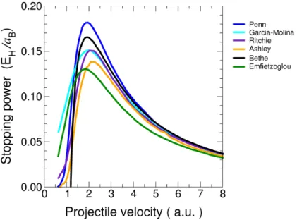
states in the fluorine-passivated silicon quantum dot and their Fourier transform……...47 Figure 3.9 - The power (phonon) spectra calculated forpassivated silicon quantum dots…...49 Figure 4.1 - The total stopping power for protons in amorphous carbon (2.0 g/cm3)…...…59 Figure 4.2 - Contemporary analytical models of the electronic stopping power
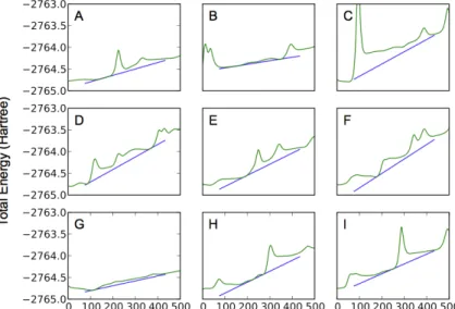
of a proton in liquid water……….65 Figure 4.3 - Baseline fitting of the change in total energy for a proton travelling at constant
velocity through liquid water………..………...72 Figure 4.4 - Convergence of the predicted stopping power of protons in liquid
water as a function of the number of random paths………..………74 Figure 4.5 - The electronic stopping power of protons in liquid water via
real-time time-dependent density functional theory simulations………..………75 Figure 4.6 - The electronic stopping power of alpha-particles in liquid water via
real-time time-dependent density functional theory simulations………..78 Figure 4.7 - First-principles calculations of mean steady-state charge state of
a proton (green) and an alpha-particle (red) traveling through liquid water…………...81 Figure 4.8 | Evaluation of the validity of linear response theory in calculating
Figure 4.9 - Estimated electronic stopping power for protons in liquid water
calculated using two hybrid exchange-correlation functionals………..………..……...85 Figure 4.10 - Sensitivity of the mean steady-state charge on a proton in liquid
water to approximations in the exchange-correlation functional………..…………86 Figure 4.11 - The non-adiabatic force and single-particle excitation probability
experienced by a proton traveling through liquid water………..………...89 Figure 4.12 - Changes to the valance band density of water via hole generation
for a proton in liquid water………..………...91 Figure 4.13 - Maximally localized Wannier functions of liquid water………...…...93 Figure 4.14 - The hole generation for three water molecules excited by a 20keV
proton in liquid and gas phases………..………..…….95 Figure 4.15 - The hole generation of a gas-phase water molecule by an energetic
proton with an effective charge of Zeff = 1 and Zeff = 0.5...………..97
Figure A.1 - A Wannier function analysis for 1-nonene……...………..…………..114 Figure B.1 - Bader analysis is performed on the electron density following an
energetic ion traveling through a slab of liquid water………..…………..117 Figure B.2 - Estimated steady-state charge associated with protons and alpha-
LIST OF ABBREVIATIONS
B3LYP Becke-3-paremeter-Lee-Yang-Parr functional
BK Brandt-Kitagawa
BLYP Becke-Lee-Yang-Parr
BO Born-Oppenheimer
CI Configurational interaction
CPA Classical path approximation
CPMD Car-Parrinello molecular dynamics
CSE Chemical state effects
DFT Density functional theory
ELF Energy loss function
FFT Fast Fourier transform
FPMD First-principles molecular dynamics FSSH Fewest-switches surface hopping GGA Generalized gradient approximation
GS Ground state
HEG Homogeneous electron gas
HF Hartree-Fock
HK Hohenberg-Kohn
ICRU International Commission on Radiation Units
KS Kohn-Sham
LC-BLYP Long-range corrected BLYP
MLWF Maximally localized Wannier function
NA Non-adiabatic
PBE Perdew-Burke-Erzerhof
PBE0 Perdew-Burke-Erzerhof with 0.25 HF exchange
PPA Plasmon-pole approximation
PSE Physical state effects
QP Quasiparticle
RK4 Fourth-order Runge-Kutta integrator
RPA Random phase approximation
RT-TDDFT Real-time time-dependent density functional theory SEP Single-particle excitation probability
SiQD Silicon quantum dot
TDKS Time-dependent Kohn-Sham
CHAPTER 1: INTRODUCTION
P=exp −1
4𝜋𝜉 Eq. 1.1
where 𝜉, the so-called Massey parameter is written as
𝜉 R = Δ𝐸 R
ℏR∙g R Eq. 1.2
The Massey parameter is determined based on the energy difference for the current nuclear configuration (Δ𝐸 R ), as well as the velocity of the atoms (R) involved in the transition. The function g R represents the coupling between the electronics wavefunctions. From the Landau-Zener expression in Eq. 1.1, a transition is more likely as 𝜉 becomes smaller. Therefore, consistent with physical intuition, the model suggests a cooperative set of conditions that lead to electronic transitions: smaller energy differences, greater atom velocities, and strong coupling between adiabatic states.
While this phenomenological model may guide intuition about the applicability of the BO adiabatic approximation, it remains limited in actually predicting the overall effect of non-adiabaticity in complex material properties in which the quantities in Eq. 1.2 may be difficult
to access. Motivated by the consideration for electronic transitions, numerous extensions of molecular dynamics (MD) simulations were developed to include quantum transitions. Arguably, the most notable example of these mixed quantum/classical simulation techniques is the surface-hopping method developed by Tully [4-6].
motion that occurs throughout the relaxation process. For example, systems in an electronic excited state relax to the electronic ground state by coupling to the motion of nuclei in the system, and thus the electron relaxation dynamics can no longer be treated independently of the system’s nuclear motion (i.e. phonon modes, bond stretching, bond bending, etc.). Additionally, systems can be excited if they are in a specific nuclear configuration in the ground state and nearest excited state approach in energy as the nuclei move. These excitations can be thermally generated or due to the transfer of energy from another source. Photodissociation, fragmentation due to ionization events, and electron-hole migration are all examples of systems where electron and nuclei dynamics are inextricably related as a result of an electronic structure that is far from the electronic ground state for a particular nuclear configuration. For these systems, the BO adiabatic approximation will consistently fail to properly describe the physics of the concerted electron and nuclear motion and in some cases fail to detect certain phenomena altogether. In order to fully describe the electron dynamics, non-adiabatic effects must be taken into account.
mitigate an effect, atomistic-detail and predictive capabilities are two highly-desirable features of an effective computational approach to exploring non-adiabatic dynamics.
Integrating these many-body, non-adiabatic effects, however, is not straightforward. While analytical expressions for non-adiabatic terms are exact in theory, they have only been calculated for smaller, simpler systems such as non-adiabatic charge transfer between two fixed ions [11]. Recent work by Abedi et al. (2016) account for this non-adiabaticity using the exact factorization approach [12,13] and appears promising for future work in simulating non-adiabatic dynamics that include both nuclear and electron dynamics. The authors note, however, that this exact formalism still only serves as a basis from which approximations must still be made for larger, complex systems. When performing first-principles simulations, however, access to sufficient computing resources and efficiently parallelized codes continue to limit the size of the systems that we can simulate non-adiabatic dynamics.
First-principles calculations offer a distinct advantage to analytical approaches, which while theoretically sound, still often rely on extensive amounts of parameterization. A first-principles approach eliminates the need for fitting parameters or experimental data and opens the approach up to being predictive. A significant portion of the discussion throughout this work will focus on the particular role that atomistic detail (e.g. surface chemistry, molecular order/disorder, chemical bonding, etc.) play in dictating electronic response. In the remainder of this work, we will discuss two important, non-adiabatic phenomena via the use of first-principles simulations.
fluorine-passivated quantum dot by an order of magnitude. We concluded that the relaxation dynamics of carriers in nanocrystalline silicon is sensitive to the chemistry at the surface for two reasons: (1) changing atoms at the surface can significantly influence the electronic structure of the entire quantum dot and (2) the differences in mass and bond strength/rigidity at the surface manifest in notably different nuclear motion at the surface which directly influences the coupling between electronic states. This is consistent with experimental work, which suggests that recombination rates within quantum dots are sensitive to stabilizing surface ligands [14-18]. This work is the subject of the paper published in Nano. Lett. 15, 6429 (2015) [19].
Next, we investigate a very different system that is nonetheless dominated by another non-adiabatic phenomenon, electronic stopping. Here we investigate the energy transfer process between high-energy ions and liquid water. This section is divided into two main sections: our quantitative and qualitative understanding of these systems. In both studies, we rely on real-time, first-principles electronic structure calculations to evolve the electronic system of the water as it is exposed to a charged particle (i.e. proton or alpha-particle) with a kinetic energy that falls within the range of 1-10MeV. Our real-time time-dependent density functional theory calculations provide information about total energy of the system, but also a three-dimensional description of the electron density of water throughout the simulation.
experiment at most velocities with a stark absence of data within the velocity regime surrounding the anticipated peak. For the first time, we present a first-principles electronic stopping power curve for a liquid condensed matter system via a series of simulations that allow us to determine the amount of energy that is transferred into the electronic subsystem via electronic excitations. This work is the subject of the paper published as a Rapid Communication in Phys. Rev. B 94 (2016) [20].
In the mixed qualitative-quantitative study of the mechanism by which these electronic excitations are generated, we simulate and focus our analysis on a single ion trajectory passing through liquid water at a velocity just below the computationally predicted peak velocity. We selected this velocity to better understand the important dynamics that occur at the Bragg peak, or roughly where the ion is depositing the maximal amount of energy into the system. Despite its importance in hadron therapies of cancer and in degeneration of materials in nuclear reactors, little is still known about the excitation and ionization that occurs. We observed that the majority of excitations that occur and that contribute to the electronic stopping are generated via ionization events that involve the water molecules nearest to the path of the ion. Electron density localized on individual molecules is excited throughout the entire system, or in other words, water molecules are ionized as the projectile passes by them. This work is the subject of an article that is currently under peer-review and is expected to be published in the Fall of 2016.
REFERENCES
[1] M. Born and R. Oppenheimer, Ann Phys-Berlin 84, 0457 (1927). [2] C. Zener, P R Soc Lond a-Conta 137, 696 (1932).
[3] L. Landau, Physikalische Zeitschrift der Sowjetunion 2, 46 (1932). [4] K. Drukker, J Comput Phys 153, 225 (1999).
[5] J. C. Tully, J Chem Phys 93, 1061 (1990).
[6] J. C. Tully and R. K. Preston, J Chem Phys 55, 562 (1971).
[7] J. A. Efstathiou, P. J. Gray, and A. L. Zietman, Brit J Cancer 108, 1225 (2013). [8] W. D. Newhauser and R. Zhang, Phys Med Biol 60, R155 (2015).
[9] J. Sisterson, Nucl Instrum Meth B 241, 713 (2005). [10] B. C. Garrett et al., Chem Rev 105, 355 (2005).
[11] F. Agostini, A. Abedi, Y. Suzuki, S. K. Min, N. T. Maitra, and E. K. U. Gross, J Chem Phys 142 (2015).
[12] A. Abedi, F. Agostini, and E. K. U. Gross, Epl-Europhys Lett 106 (2014). [13] A. Abedi, N. T. Maitra, and E. K. U. Gross, Phys Rev Lett 105 (2010).
[14] M. T. Frederick, V. A. Amin, and E. A. Weiss, J. Phys. Chem. Lett. 4, 634 (2013). [15] S. Y. Jin, R. D. Harris, B. Lau, K. O. Aruda, V. A. Amin, and E. A. Weiss, Nano Lett
14, 5323 (2014).
[16] K. E. Knowles, M. T. Frederick, D. B. Tice, A. J. Morris-Cohen, and E. A. Weiss, J. Phys. Chem. Lett. 3, 18 (2012).
[17] M. Malicki, K. E. Knowles, and E. A. Weiss, Chem. Commun. 49, 4400 (2013). [18] M. D. Peterson, L. C. Cass, R. D. Harris, K. Edme, K. Sung, and E. A. Weiss, Annu.
Rev. Phys. Chem. 65, 317 (2014).
CHAPTER 2: THEORETICAL BACKGROUND AND NUMERICAL METHODS
2.1 Electronic Structure Theory
the vast computing resources most effectively. The following chapter includes both the theoretical background relevant to this dissertation as well as the methods by which simulations and calculations are performed. Throughout this text, we make use of atomic units such that 𝑒!,𝑚, and ℏ are all unity.
2.1.1 Density Functional Theory
In a system where we apply the Born-Oppenheimer adiabatic approximation [1], we are interested in determining the ground state electronic structure for a given, unchanging configuration of nuclei. The equation that describes the quantum-mechanical behavior of electrons in these stationary states is the time-independent, electronic Schrödinger equation, written here as
−ℏ
!∇
!!
2𝑚! + 𝑣 r!; R! +
!
!!!
!
!!!
𝑤 r!,r! +
!
!,!
!!!
Ψ! r!,⋯,r!;R!,⋯,R!
= ε!Ψ! r!,⋯,r!;R!,⋯,R! Eq. 2.1
where 𝑣 r! is some external potential that depends parametrically on the position of the systems nuclei R! and 𝑤 r!,r! represents the interaction between electrons.
of particles—into a set of coupled, lower-dimensional wave functions. The HK proof reasoned via a proof by contradiction that for an interacting system of N electrons in an external potential 𝑣!"# r that varies by more than a constant, there exists a one-to-one correspondence between that potential and the ground state electron density 𝑛! r [21]. Even more powerfully, it follows that the non-degenerate ground state (GS) many-body wave function is a functional of the ground state density Ψ! X!,⋯,X! =Ψ! 𝑛! r . Access to the many-body wave function implies that any physical observable, O, also has a functional form via O 𝑛! r = Ψ! 𝑛! r 𝑂 Ψ! 𝑛! r . The total energy (E) of a ground-state electronic system is that system’s minimum, and thus the approach up until this point, was to vary 𝑛! r so as to minimize 𝐸 𝑛! r . The minimization of the total energy is often performed via a constrained search based on work by Levy [22,23] and Lieb [24]. The total energy can be written as
𝐸 = Ψ 𝑇Ψ + Ψ 𝑣ee Ψ + 𝑑!r 𝑣
ext r 𝑛 r Eq. 2.2
where 𝑇 is the kinetic energy operator for the electrons, 𝑣ee is the electron-electron
𝐹 𝑛 r = min
!→!r Ψ 𝑇+𝑣ee Ψ Eq. 2.3
The total energy, 𝐸, therefore becomes a functional of the electron density, and the ground state electron density can be determined as expressed in Eq. 2.3 by minimizing 𝐸 through variations in 𝑛(r).
𝐸 𝑛 r = min
! 𝐹 𝑛 r + 𝑑
!r 𝑣
ext r 𝑛 r Eq. 2.4
It should be noted at this point, however, that the exact expression for 𝐹[𝑛(r)] remains unknown and is the source of continued work on modern density functional theory.
It would be a year following the HK proof that Kohn and Sham (KS) [25] would propose a formulation of density functional theory (DFT) that is used today [26]. The KS system is defined to be the fictitious system of non-interacting, single-particle wavefunction where the electron density is identical to that of the interacting system and is expressed as 𝑛 r =
𝜑! r !
!
!!! where 𝜑! r is the set of KS orbitals. Each single-particle orbital is governed by the expression
−1
2∇!+𝑣ext r + 𝑑!r 𝑛 r
r-‐r' +𝑣XC 𝑛 r 𝜑! r = 𝜀!𝜑! r Eq. 2.5
where
𝑣XC 𝑛 r = 𝛿𝐸XC
and 𝐸XC is the exchange-correlation (XC) energy which is a functional of the electron density. The final three terms within the brackets of Eq. 2.5 represent the Kohn-Sham potential, which represents the unique potential experienced by non-interacting electrons that corresponds exactly to the ground-state electron density described by the interacting, many-body wavefunction. All many-body effects are captured in the XC functional. The exact form of this functional is unknown, however, and there exist many different approximations to the functional. Among the most commonly used functionals is the local density approximation (LDA, 𝐸XC!"# 𝑛 r ) which approximates the XC energy of the total system as a sum of
approach. Parr and Yang in addition to Lee and Becke at this time would also contribute the Becke-Lee-Yang-Parr (BLYP) [29], a gradient-corrected functional that showed some of the first promising DFT calculations of atoms and small molecules. A second common GGA functional is the Perdew-Burke- Ernzerhof (PBE) XC functional [30]. The PBE functional was constructed specifically to meet several criteria required within DFT including the Lieb-Oxford bound, which requires that the exchange energy alone for a given density is greater than or equal to that of the exchange-correlation energy for the same density [31], and the correct linear response of the uniform electron gas [32].
number of electrons in the system, 𝒪 𝑁!! . This is compared to the 𝒪 𝑁!! scaling of HF to evaluate the four-center, two-electron integrals necessary to compute the exact exchange. As of today, in most cases hybrid functionals cannot be utilized in calculations of systems with large numbers of electrons.
First-Principles Molecular Dynamics
Classical molecular dynamics is a well-established field where the interatomic interactions are described by potentials created before any simulation is ever run [41,42]. Classical molecular dynamics has been used widely in chemistry, physics, materials science and more recently in biochemistry and biophysics. Despite these successes in reproducing these and other experimental data, classical simulations do have their limitations. For example, there is an assumption that interactions that are predefined between particles are well suited for atoms in all environments, simple or complex. Similarly, there is an assumption that the interactions experienced by an atom throughout the simulation are static, as most classical potentials remain unchanged in their formulaic expression throughout the simulations. In some cases, potentials are parameterized according to experimental measurements or according to a variety of other schemes in order to account for differences in complex, chemical systems [43]. This approach, however, significantly limits the method to being fully predictive and requires that a system be synthesized in order to simulate its behavior. Finally, classical molecular dynamic has the known challenge of properly describing bond-breaking and bond-making. Often, force fields will impede changes to chemical bonding or poorly describe the new system.
instead of predefining the potentials used throughout the simulation, the forces acting on the nuclei are calculated on-the-fly using electronic structure theory. Throughout this work, we will discuss the use of DFT to determine the ground state electronic structure necessary to compute forces acting on nuclei, however other electronic structure methods could also be used. We discuss and utilize DFT in particular because it has proven to be both an effective and computationally affordable approach to determine the electronic structure of stationary electronic states for large and complex molecular systems. The disadvantage to this approach is the computational cost associated with performing a ground-state calculation at each time step throughout the simulation.
One assumption that is regularly made which is generally valid for many chemical systems is the Born-Oppenheimer (BO) adiabatic approximation. Succinctly stated, this assumption assumes that the motion of the electrons is entirely decoupled from the motion of the nuclei. Nuclei evolve in time with forces determined by the ground-state electronic structure for the given atomic configuration. Thus, the general approach of ab-initio molecular dynamics is to calculate the ground-state electronic system based on a specific configuration of nuclei from first-principles electronic structure calculations, and to advance the classical nuclei using Newton’s equations of motion where forces are determined from the ground state electronic structure. The Hellman-Feynman force [44] acting on each ion, I, is calculated in Eq. 2.7
𝑀!R! = − Ψ! ∇!ℋ! Ψ! Eq. 2.8
where ∇! is the gradient in the electronic coordinates based on a displacement in the ion I. Ψ!
is the ground-state many-body electronic wavefunction, which in the cases of DFT is a Slater determinant of the single-particle, ground-state KS-orbitals. Eq. 2.8 offers a slightly different representation of Eq. 2.7 where the force is related to the mass and acceleration of the nucleus. Work by Feynman [44] notes that the right-hand expression in Eq. 2.7 simplifies to Eq. 2.8 if the many-body wavefunction is an eigenfunction or a linear combination of eigenfunctions of the electronic Hamiltonian, ℋ!. In the case of KS DFT, ℋ! is the KS Hamiltonian and the forces can be determined for a specific nuclear configuration by evaluating the expression ∇!ℋ!KS.
Algorithms used to integrate Newton’s equations of motion vary widely, although some of the most common algorithms include Verlet algorithm [45], the Leap Frog algorithm [46] and the Euler algorithm [46]. The choice of each algorithm influences the time step that is appropriate to accurately capture dynamics. Time steps of ~1fs, for example, are commonly used in FPMD to generate accurate simulations of 1ps-10ps in length, long enough to generate statistics in agreement with experimental measurements.
Quantum Dynamics: Beyond Ground-State Dynamics
approximation, these processes, which include electron transfer [47], phonon-induced carrier relaxation [48-51] and exciton dynamics [52,53], require an approach that takes into consideration the connection between electron and nuclear dynamics (i.e. non-adiabatic effects). While the BO adiabatic approximation provides a significant simplification to simulations, incorporating non-adiabaticity into simulations leads to a significant increase in both the cost and the complexity of the computations. The following sections represent two well-accepted theoretical approaches to capture non-adiabatic dynamics in molecular simulations: fewest-switches surface hopping (FSSH) and real-time time-dependent density functional theory (RT-TDDFT).
2.1.2 Fewest-Switches Surface Hopping
between potential energy surfaces (a “hop”) between adiabatic states is determined based on a phenomenomlogical hopping criterion. If a hop occurs, the active surface is redefined. In the original formulation of surface hopping, there were an indefinite number of hops that a particle could make between surfaces. It wouldn’t be until 1990 that Tully would propose the FSSH algorithm as a means to minimize the number of hops between potential energy surfaces [5]. When not minimized, the excessive hopping outside of the region of the electronic crossings essentially lead to dynamics that are more similar to a weighted-average of the two adiabatic stats, and can lead to unphysical dynamics outside of the electronic crossings [4]. The FSSH hopping criterion is derived specifically to limit the electronic hops to the region of strong non-adiabatic coupling (i.e. electronic crossings). FSSH has been shown to capture the correct dynamics for non-adiabatic dynamics such as carrier recombination [55], photochemistry [56], and phonon-assisted carrier relaxation [5].
The FSSH algorithm can also be extended into a formulation based on single-particle wavefunctions as proposed by Prezhdo [57-59]. Instead of hops between many-body adiabatic states as was the case in Tully’s surface hopping, Prezhdo proposed the use of single-particle wavefunctions as states to and from which electrons might hop. Single-particle wavefunctions are evolved in time according to the set of coupled, time-dependent Kohn-Sham (TDKS) equations, where 𝜑! are the corresponding single-particle KS orbitals.
𝑖ℏ𝜕𝜑!𝜕𝑡r,𝑡 =ℋKS 𝜑
It should be noted that KS Hamiltonian depends on the electronic density via the occupied, TDKS orbitals. We can alternatively express the time-dependent wavefunctions in the adiabatic KS orbitals (ground state KS-orbitals, 𝜑! ).
𝜑! r,𝑡 = 𝑐!" 𝑡 𝜑! r;R
!!
!!!
Eq. 2.10
Here, 𝑐!" 𝑡 are the time-dependent coefficients that relate the adiabatic KS orbitals to the time-dependent wavefunctions, calculated as 𝜑! r 𝜑! r,𝑡 . Substituting Eq. 2.10 into Eq. 2.9, multiplying by a single adiabatic state from the left and integrating leaves the following expression and its approximation.
𝑖ℏ𝜕𝑐!" 𝑡
𝜕𝑡 = 𝑐!" 𝑡 𝜑! r;R ℋKS 𝜑! 𝜑! r;R +d!"∙R
!!
!!!
Eq. 2.11
𝑖ℏ𝜕𝑐𝜕𝑡!" 𝑡 ≈ 𝑐!" 𝑡 𝜀!𝛿!"+d!"∙R
!!
!!!
Eq. 2.12
time-dependent electron density does not deviate significantly from that density generated by the adiabatic states, then the approximation ℋKS 𝜑
! 𝜑! r;R ≈ℋKS 𝜑! 𝜑! r;R =
𝜀!𝜑! r;R remains reasonable and Eq. 2.11 can be simplified to Eq. 2.12. The second term in
the brackets in the right-hand side of Eq. 2.11 refers to d!" and the non-adiabatic (NA)
coupling term. The NA coupling relates the coupling of single-particle electronic states as mediated by the motion of the system’s nuclei. It is expressed as
d!"∙R=−𝑖ℏ 𝜑! r;R ∇R 𝜑! r;R ∙R=−𝑖ℏ 𝜑!
𝜕
𝜕𝑡 𝜑! Eq. 2.13
where ∇R is the gradient with respect to nuclear displacements. The expression can be rewritten in terms of a partial derivative with respect to time
d!" =
𝜑! ∇Rℋ 𝜑!
𝜀!−𝜀! ∙R Eq. 2.14
The probability of hopping between time-dependent, TDKS orbitals [60] is expressed as
P!"(𝑡,∆𝑡) =max 0,
𝑏!"∆𝑡
𝑎!! 𝑡 𝐵!" 𝑡 Eq. 2.15
where
𝑏!" =−2Re 𝑎!"∗ d
𝑎!" 𝑡 = 𝑐!𝑐!∗ Eq. 2.17
𝐵!" 𝑡 = exp
− 𝜀! 𝑡 −𝜀! 𝑡 𝑘!𝑇 1
𝜀 𝜀!> 𝜀!
!≤ 𝜀! Eq. 2.18
The probability to hop is related to several parameters including the size of the time step (∆𝑡) as well as the current occupation of the state from which the particle is hopping (𝑎!! 𝑡 ). The coupling between single-particle orbitals is captured in the expression for 𝑏!" in which the coherence between the states 𝑎!"∗ is multiplied by the NA-coupling and the current motion of the nuclei. The right-hand expression for d!"∙R in Eq. 2.13 is used to calculate 𝑏!". If 𝑏!" is computed to be negative, the probability for a hop is deemed to be impossible, and P!" =0. Detail balance is captured in FSSH by weighting the probability of a hop by a Boltzmann factor, 𝐵!" 𝑡 (see Eq. 2.15) [61]. Hops to electronic states of greater energy are therefore less
likely by including this Boltzmann factor. The time-dependence of this parameter comes in by determining the energy difference between states according to the time-dependent eigenvalues calculated on-the-fly.
complicated expression for ∇R 𝜑! r;R . The eigenvalues for each step in the FSSH calculation correspond to those computed on-the-fly during the FPMD.
Surface hopping does have its limitations, however, which should be acknowledged. First is the challenge of decoherence. The FSSH algorithm has the well know challenge of inaccurately propagating electronic wavefunctions on different electronic surface with complete coherence (i.e. in phase). This inaccuracy can be understood simply through considering the mixed quantum-classical system in parallel to the Schrödinger’s cat. If a classical measurement is made on a superposition of quantum mechanical states, the state collapses into a pure state. The nuclei in FSSH simulations are treated classically, and so therefore these classical particles should regularly be making measurements on the quantum electronic system. The expected long-term behavior is therefore that the electronic density matrix collapses to a pure state. Evolving with complete coherence will never achieve this. This failure, however, generated little error on short timescales, but long-time dynamics can fail catastrophically. There is a growing body of work, however, to correct for this over coherence [54,63,64]. Prezhdo et al. recently proposed and extension to the FSSH algorithm to include an ad hoc decoherence time decay constant to update the electron density matrix by either collapsing or projecting out individual, adiabatic states from the state vector evolving in real time [65]. Most recently, work by Subotnik et al. have developed and implemented the so-called A-FSSH, a parameter-free approach to including decoherence correction in real time [66].
that the motion of the nuclei of our system experiencing non-equilibrium electron dynamics does not deviate significantly from the trajectories expected within the BO adiabatic approximation and therefore are assumed to be identical. In single-molecule systems, the CPA can catastrophically fail as small changes to the electronic structure are confined to a smaller area and thus can dramatically change the Columbic forces experienced by the nuclei throughout the simulation. As the system size increases, however, the CPA becomes a more reasonable approximation because the electronic feedback with the nuclei influences the nuclear trajectories to an increasingly less extent, particularly when excitations are delocalized and changes to the local electron density are minimized.
2.1.3 Real-Time Time-Dependent Density Functional Theory
to compute the excitation energies of a system [68]. This formalism can only be used when the perturbation is small and the changes in electron density do not dramatically change the overall electronic structure.
To make these many-body equations accessible, a proof similar to the Hohenberg-Kohn theorem that accounts for time dependence is necessary. It was the Runge-Gross theorem [67] in 1984 that served as proof that there indeed exists a one-to-one correspondence between densities and potentials for a given fixed initial state. Taking a similar form as the time-dependent Schrödinger equation, the time-dependent Kohn-Sham (TDKS) equations are
𝑖ℏ 𝜕
𝜕𝑡𝜓! r,𝑡 = −
ℏ!
2𝑚∇!+𝑣ext r,𝑡 + 𝑑!r 𝑛 r
r-r'
+𝑣XC 𝑛 𝑡 r 𝜓! r,𝑡
Eq. 2.19
As was true for the time-independent case, the relationship between electron density and TDKS orbital is 𝑛 r,𝑡 = !! 𝜓! r,𝑡 !
!!! . Here, the XC potential is a functional of the time-dependent density. (Further discussion regarding the XC potential in RT-TDDFT is provided below.) Provided an initial set of KS orbitals 𝜓! , RT-TDDFT simulates the dynamics of the system by propagating these 𝑁! single-particle, nonlinear TDKS equations by applying the time-evolution operator
𝜓! r,𝑇 = 𝒯exp −𝑖 𝑑𝜏 !
!
𝐻!" 𝜏 𝜓
where 𝒯 is the time-ordering operator, and 𝜓! r,𝑡 =0 represents the initial set of KS orbitals. At this point, it is worthwhile to reiterate that these coupled equations are non-linear as the KS Hamiltonian is a functional of the electron density as determined by the TDKS orbitals. The solution to Eq. 2.20 becomes essentially intractable. In practice, this propagation is performed using numerical approximations. The propagation scheme used to evolve a set of TDKS equations depends on a variety of factors including the basis set representation and the time-step taken throughout the simulation. For example, in the Octopus code [69], which is calculated on a real-space mesh, the Crank-Nicholson (Cayley) scheme [70] and Magnus expansions [71] are both used to propagate the TDKS equations. In codes that use a planewave basis such as the Qbox/Qb@ll code[72,73], the 4th-order Runge-Kutta propagation scheme was found to be most stable and scalable to systems of thousands of electrons [74].
Exchange-Correlation Functionals in RT-TDDFT
Hartree-Fock exchange integral is gradually turned on for long-range distances using a standard error function. As can be expected with the computation of the double integral, the computational cost of Hartree-Fock limits the use of these class of XC functionals.
An additional approximation within applications of RT-TDDFT is the use of the adiabatic exchange-correlation approximation [76,77]. Eq. 2.19 indicates that 𝑣XC 𝑛 𝑡 r is a functional of the time-dependent density, and more specifically the instantaneous electron density. The development of XC potential functionals has been formulated based on ground-state DFT and as was mentioned above, uses the homogeneous electron gas as the reference to describe electron correlation. In strong fields that drive large excitations, however, it is less clear whether or not these ground-state functionals are reasonably constructed for non-equilibrium, excited-state electron densities. In particular, this critique comes from work showing that the KS potential depends on the history of the density (i.e. how the excited electron density was generated) [77]. Work has continued to incorporate history effects
(𝑡 < 𝑡’) into the XC-potential functions themselves as well as testing the contexts in which the adiabatic approximation performs with reasonable accuracy [78-82].
Computational Resources and Code Parallelization
It cannot go unstated that the feasibility of these real-time electron dynamic simulations go beyond just the theory and require an intentional consideration of the computational resources and the parallelization of the electronic structure code. The work contained within Chapter 4 (‘Electronic Stopping in Water’) makes use of the Qbox/Qb@ll code [72,73], which has been optimized to perform large-scale simulations on massively-parallel, multi-core supercomputers [83]. As a plane-wave based code (𝜓! r,𝑡 = !
! G𝐶! G,𝑡 𝑒𝑥𝑝 𝑖G∙r ,
Blue Gene/Q architecture by distributing the expansion coefficients , 𝐶! G,𝑡 , on a process
REFERENCES
[1] M. Born and R. Oppenheimer, Ann Phys-Berlin 84, 0457 (1927). [2] C. Zener, P R Soc Lond a-Conta 137, 696 (1932).
[3] L. Landau, Physikalische Zeitschrift der Sowjetunion 2, 46 (1932). [4] K. Drukker, J Comput Phys 153, 225 (1999).
[5] J. C. Tully, J Chem Phys 93, 1061 (1990).
[6] J. C. Tully and R. K. Preston, J Chem Phys 55, 562 (1971). [21] P. Hohenberg and W. Kohn, Phys Rev B 136, B864 (1964). [22] M. Levy, P Natl Acad Sci USA 76, 6062 (1979).
[23] M. Levy, Phys Rev A 26, 1200 (1982).
[24] E. H. Lieb, Int J Quantum Chem 24, 243 (1983). [25] W. Kohn and L. J. Sham, Phys Rev 140, 1133 (1965).
[26] R. G. Parr, in Horizons of Quantum Chemistry: Proceedings of the Third International Congress of Quantum Chemistry Held at Kyoto, Japan, October 29 - November 3, 1979, edited by K. Fukui, and B. Pullman (Springer Netherlands, Dordrecht, 1980), pp. 5.
[27] J. P. Perdew and K. Burke, Int J Quantum Chem 57, 309 (1996).
[28] R. M. Martin, Electronic Structure: Basic Theory and Practical Methods (Cambridge University Press, 2004).
[29] A. D. Becke, Phys Rev A 38, 3098 (1988).
[30] J. P. Perdew, K. Burke, and M. Ernzerhof, Phys Rev Lett 77, 3865 (1996). [31] E. H. Lieb and S. Oxford, Int J Quantum Chem 19, 427 (1981).
[32] M. Levy, Int J Quantum Chem, 617 (1989).
[33] P. J. Stephens, F. J. Devlin, C. F. Chabalowski, and M. J. Frisch, J Phys Chem-Us 98, 11623 (1994).
[34] C. Adamo and V. Barone, J Chem Phys 110, 6158 (1999).
[36] J. Paier, M. Marsman, and G. Kresse, Phys Rev B 78 (2008). [37] J. Heyd and G. E. Scuseria, J Chem Phys 121, 1187 (2004).
[38] E. N. Brothers, A. F. Izmaylov, J. O. Normand, V. Barone, and G. E. Scuseria, J Chem Phys 129 (2008).
[39] P. G. Moses, M. S. Miao, Q. M. Yan, and C. G. Van de Walle, J Chem Phys 134
(2011).
[40] M. Jain, J. R. Chelikowsky, and S. G. Louie, Phys Rev Lett 107 (2011).
[41] M. C. Payne, M. P. Teter, D. C. Allan, T. A. Arias, and J. D. Joannopoulos, Rev Mod Phys 64, 1045 (1992).
[42] D. K. Remler and P. A. Madden, Mol Phys 70, 921 (1990).
[43] L. Monticelli and D. P. Tieleman, in Biomolecular Simulations: Methods and Protocols, edited by L. Monticelli, and E. Salonen (Humana Press, Totowa, NJ, 2013), pp. 197.
[44] R. P. Feynman, Phys Rev 56, 340 (1939). [45] L. Verlet, Phys Rev 159, 98 (1967).
[46] D. Frenkel and B. Smit, Understanding Molecular Simulation: From Algorithms to Applications (Academic Press, 2002), Vol. 1, Computational Science: From Theory to Applications.
[47] W. R. Duncan and O. V. Prezhdo, Annual Review of Physical Chemistry 58, 143 (2007).
[48] Y. G. Semenov and K. W. Kim, Phys Rev Lett 92 (2004).
[49] E. A. Muljarov, T. Takagahara, and R. Zimmermann, Phys Rev Lett 95 (2005). [50] M. Califano, A. Zunger, and A. Franceschetti, Nano Lett 4, 525 (2004).
[51] D. S. Kilin, O. V. Prezhdo, and M. Schreiber, J Phys Chem A 111, 10212 (2007). [52] A. B. Madrid, K. Hyeon-Deuk, B. F. Habenicht, and O. V. Prezhdo, ACS Nano 3,
2487 (2009).
[53] C. Sousa, S. Tosoni, and F. Illas, Chem Rev 113, 4456 (2013).
[54] J. E. Subotnik, A. Jain, B. Landry, A. Petit, W. J. Ouyang, and N. Bellonzi, Annu Rev Phys Chem 67, 387 (2016).
[56] E. Tapavicza, G. D. Bellchambers, J. C. Vincent, and F. Furche, Phys Chem Chem Phys 15, 18336 (2013).
[57] O. Prezhdo, Abstr Pap Am Chem S 244 (2012). [58] O. Prezhdo, Abstr Pap Am Chem S 243 (2012). [59] O. V. Prezhdo, Abstr Pap Am Chem S 238 (2009).
[60] L. J. Wang, R. Long, and O. V. Prezhdo, Annual Review of Physical Chemistry, Vol 66 66, 549 (2015).
[61] P. V. Parandekar and J. C. Tully, J Chem Phys 122 (2005).
[62] S. Hammes-Schiffer and J. C. Tully, J Chem Phys 101, 4657 (1994). [63] B. R. Landry and J. E. Subotnik, J Chem Phys 137 (2012).
[64] B. R. Landry and J. E. Subotnik, J Chem Phys 135 (2011).
[65] H. M. Jaeger, S. Fischer, and O. V. Prezhdo, J Chem Phys 137 (2012). [66] N. Shenvi, J. E. Subotnik, and W. T. Yang, J Chem Phys 134 (2011). [67] E. Runge and E. K. U. Gross, Phys Rev Lett 52, 997 (1984).
[68] C. Ullrich, Time-dependent density-functional theory : concepts and applications (Oxford University Press, Oxford ; New York, 2012), Oxford graduate texts.
[69] X. Andrade et al., Phys Chem Chem Phys 17, 31371 (2015).
[70] W. H. Press, Numerical recipes : the art of scientific computing (Cambridge University Press, Cambridge, UK ; New York, 2007), 3rd edn.
[71] W. Magnus, Commun Pur Appl Math 7, 649 (1954).
[72] E. W. Draeger and F. Gygi, Lawrence Livermore National Lab, Qbox (Qb@ll Branch), tech. report, (2014).
[73] F. Gygi, Ibm J Res Dev 52, 137 (2008).
[74] A. Schleife, E. W. Draeger, Y. Kanai, and A. A. Correa, J Chem Phys 137 (2012). [75] H. Iikura, T. Tsuneda, T. Yanai, and K. Hirao, J Chem Phys 115, 3540 (2001). [76] N. T. Maitra, Abstr Pap Am Chem S 228, U260 (2004).
[78] J. F. Dobson, Phys Rev Lett 73, 2244 (1994).
[79] J. F. Dobson, M. J. Bunner, and E. K. U. Gross, Phys Rev Lett 79, 1905 (1997). [80] E. K. U. Gross and W. Kohn, Phys Rev Lett 55, 2850 (1985).
[81] G. Vignale and W. Kohn, Phys Rev Lett 77, 2037 (1996).
[82] G. Vignale, C. A. Ullrich, and S. Conti, Phys Rev Lett 79, 4878 (1997).
CHAPTER 3 : EXCITED ELECTRON RELAXATION - THE ROLE OF SURFACE PASSIVATION IN SILICON
3.1 Overview
chapter, we discuss the role that surface passivation of a silicon quantum dot plays in the system’s electron relaxation dynamics. Here, we choose to study silicon because of its ubiquity in electronic technologies. Additionally, the extensive work with silicon has led to a significant amount of synthetic control allowing us to simulate systems that echo experimental work generating nanometer-sized nanocrystal and controlling chemically passivated surfaces. We apply fewest-switches surface hopping, a mixed quantum/classical approach, to capture the non-adiabatic dynamics of the relaxation process.
3.2 Numerical Details
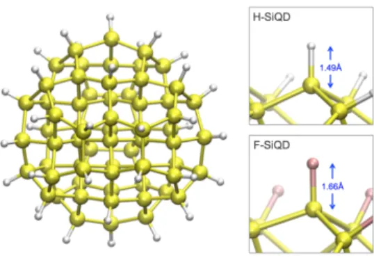
In this work, we consider a small, well-defined silicon quantum dot approximately 1.5 nm in diameter. On the surface of each quantum dot (66 silicon atoms), a layer of 40 passivating atoms was arranged such that no silicon dangling bonds existed. The structure for each dot can be seen in Figure 3.1. Density functional theory was use to optimize the
Figure 3.1 | The initial atomic configuration of the silicon nanocrystal. The structure contains sixty-six silicon atoms and forty passivating atoms. The hydrogen-passivated silicon quantum dot has an average bond length of 1.49Å while the fluorine-passivated silicon quantum dot has an average bond length of 1.66Å.
Density Functional Theory Calculations and First-Principles Molecular Dynamics
small size of the system and limitations in the fewest-switches surface hopping (FSSH) code, only a Γ-point calculation was performed in Qbox.
At the beginning of the simulation, the velocities of the nuclei were initially randomized while conserving the total kinetic energy (i.e. temperature). This was done in order to remove any collective motion inadvertently imparted on the system during the relaxation process. The temperature of the system was kept constant using the “scaling” thermostat implemented in Qbox. This thermostat rescales the velocities of all atoms according to the expression 𝑣! = 𝑣! 1−𝜂𝑑𝑡 , where 𝜂 =𝜏!!tanh 𝑇−𝑇
!"# /∆ . In the previous expression, 𝜏 is the thermostat time constant set to 24.189fs and ∆ is the thermostat temperature window set to 100K. All simulations used a 𝑇!"# of 295K. The calculation was performed using a time step of 0.5fs. Throughout the simulation, the non-adiabatic coupling (NA-coupling) matrix was calculated numerically on-the-fly during the FPMD via the approach proposed by Hammes-Schiffer and Tully[62]. This approach applies a finite differences approach to Kohn-Sham wave functions of adjacent time steps and pays particularly close attention to the phase of the electronic states. FPMD simulations were generated for each dot for a total of 1.25 ps each, or a total of 2500 molecular dynamics steps.
Fewest-Switches Surface Hopping Calculations
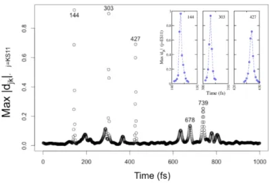
step of 0.5fs was determined to be sufficiently small to calculate converged NA-couplings. In
Figure 3.2, the NA-coupling for an electronic state is plotted throughout he simulations. It is
clear that a time step of 0.5fs indeed captures the sharp peaks in the NA-couplings. Additionally, the 1.25ps FPMD simulations were found to be long enough to adequately capture both high and low frequency and vibrational modes in each system.
Figure 3.2 | The maximum non-adiabatic (NA) coupling calculated between the eleventh unoccupied KS orbital and all other KS orbitals throughout the duration of the FPMD simulation. The inset shows zoomed in regions for each peak in NA-coupling. Similar temporal resolution was observed for the maxima of other KS orbitals.
relaxation time constants from the initially populated states were considerably under-predicted by an order of magnitude. To account for the motion of the ions, we apply the classical path approximation (CPA). We set a decoherence time constant of 10000 a.u. such that during our simulations, the ad hoc decay of off-diagonal elements in the density matrix to correct the overcoherence of FSSH are not applied.
3.3 Results and Discussion
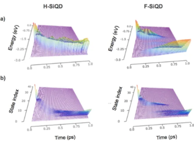
When calculating the relaxation dynamics using the method proposed by Prezhdo et al. [93], there are two distinct representations of the analysis: electron relaxation through electronic state indices and relaxation according to the energy of a particle above the system’s valance band edge (Figure 3.3). These representations provide two important yet
different perspectives to the analysis.
Figure 3.3 | Two representations of the hot carrier relaxation process as determined by fewest-switches surface hopping (FSSH) calculations. Representations are presented for a hydrogen-passivated silicon quantum dot (H-SiQD, left) and a fluorine-passivated silicon quantum dot (F-SiQD, right). Relaxation can be visualized via energetics (top row) or via electronic state index (bottom row).
As is evident from Figure 3.3, the features between the two representations do not change
factor that is entirely missing from the electronic state index but captured in the energy representation. In the energy representation, the populations of two states of similar energy will sum to create a stronger feature than in the index representation where states remain separated along the y-axis of the plot. Information about the density of states is implicitly included in the energy representation because electronic populations will only exist on the energy axis where there are also electronic states. One advantage of the energy representation is that an average energy of the electron can be approximated for the excitation. In this representation, however, the details of how individual electronic states participate in the dynamics are lost and therefore the mechanism may remain obscured. Alternatively, representing the relaxation process using the electronic state indices allows us to identify contributions from individual states, but we lose valuable information about the energetics of the process. In the remainder of this work, we choose to represent the relaxation dynamics in the electronic state index representation. While the energy representations were consulted throughout the analysis, the purpose of this work was to identify and explain features within the relaxation process; therefore to capture the details of the mechanism the use of electronic state indices are a more intuitive choice.
3.3.1 Dynamics of hydrogen-passivated dot
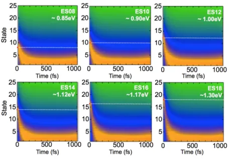
In Figure 3.4, we present six surface hopping simulations in which we varied the electronic
Figure 3.4 | Population changes for a hydrogen-passivated silicon quantum dot (H-SiQD). Initially-populated states range from ~0.85eV to ~1.30eV. The dotted, white line indicates the state in which the excited electron is initially populated.
In each plot, we observe that the excited electron relaxes to a Boltzmann distribution within ~100fs regardless of the initial excited-state energy. From the analysis, we note that there is very little sensitivity of the relaxation dynamics based on which initial state in the hydrogen-passivated quantum dot is populated.
3.3.2 Dynamics of Fluorine-Passivated Dot
Figure 3.5 | Population changes for a fluorine-passivated silicon quantum dot (F-SiQD). Initially-populated states range from ~0.56eV to ~1.18eV. The dotted, white line indicates the state in which the excited electron is initially populated.
In Figure 3.5, excited electrons that have energies greater than ~0.75eV above the LUMO
interact with a unique set of states that leads to a feature that creates a bottleneck in the relaxation dynamics that is not present in the hydrogen-passivated case. The slowed relaxation dynamics led to a relaxation process that is extended by hundreds of femtoseconds compared to the analogous, hydrogen-passivated system. Our investigation thus shifts to understanding the relationship between this unique feature and the dynamical electronic structure of these nanoscale systems. We identified that it is the eleventh unoccupied KS electronic state (ES11) as the state above which these slowed dynamics of the excited electron can be observed. This state is independent of the choice of initial state, as long as the initial state falls above ES11.
Visualizing the Quantum Dots’ Electronic Structure
[14,15,17,18], and therefore during synthesis, close attention is paid to materials’ surface quality and inadvertent inclusions of impurities or vacancies.
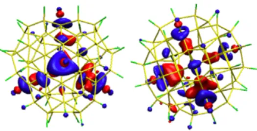
Figure 3.6 | The electronic isosurface for the eleventh unoccupied single-particle electronic state (ES11) of the fluorine-passivated silicon quantum dot (F-SiQD) in its equilibrium geometry. The two orientations of the same system show the high tetrahedral symmetry of the electronic state.
In our simulations, however, we prepare pure materials with a completely passivated surface such that no silicon dangling bonds remained at the surface. Density functional theory allows us to visualize the electron density of an individual single-particle electronic state according to the relationship 𝜌! r = 𝜓! r ! where 𝜓
do note that there is unusually high amount of tetrahedral symmetry for ES11 (Figure 3.6) and
that, while fluctuating in response to the nuclear motion, the symmetry persists throughout the entire simulation. By visual inspection of the electron density and spatial extent of the electronic wave functions alone, the explanation for the slower relaxation remains unclear.
Figure 3.7| Distribution of the non-adiabatic couplings throughout the FPMD performed on the fluorine-passivated silicon quantum dot. Each distribution includes the magnitude of the NA-coupling for states with an index ±1.
Distribution of Non-adiabatic Couplings
Given that the NA-couplings determine the non-adiabatic dynamics, we next investigate the distributions of NA-couplings for each state to identify any trends that might explain the bottleneck observed at ES11. Figure 3.7 shows the distributions of the NA-couplings for the
fluorine-passivated SiQD and each state indicated alongside the distribution. As mentioned in Chapter 2, the NA-coupling matrix decays to zero for off-diagonal elements far from the diagonal. For this reason, the distributions shown in Figure 3.7 are only for electronic states
d!" tends to zero) for electronic states ES10 and ES11. It is also clear that there are some non-zero NA-couplings which implies that, although weakly, coupling does still happen between adjacent states.
To better understand the physical reason for this poor coupling, we refer back to Eq. 2.14, which expresses the NA-coupling between two electronic states as having contributions from both the character of the wave function as well as the energetic separation between the states. Quantifying and analyzing the numerator of Eq. 2.14 is not possible given the available tools implemented into the electronic structure code at the time of this study, but it should be noted that our visual inspection of the wave functions indicated that the poor coupling was not likely due to the presence of highly localized states and therefore poor spatial overlap. We are able, however, to extend our analysis by investigating the energy differences between adjacent states. The NA-coupling between two electronic states is inversely related to the total energy between those states. Thus, visualizing the distribution of energy differences between adjacent states throughout the duration of the simulation can provide some measure for how the NA-couplings fluctuate based only on the energetics of the simulation. These energy differences are plotted in Figure 3.8a. From this distribution, we notice that the energy
which excited electron density in ES12 can couple to lower energy states. Thus, ES11 serves essentially to shuttle the electronic population over a large energy gap (~0.3eV) from ES12 to ES10. After publication of this work on the non-adiabatic dynamics in silicon quantum dots [19], Lim et al. reported a similar dynamical gap state in bulk silicon during their simulation of the non-adiabatic dynamics generated via self-irradiation [94].
(A) (B)
Figure 3.8| (A): Oscillations of the energy differences between unoccupied electronic states in the fluorine-passivated silicon quantum dot (F-SiQD). Differences between ES8 and ES9 are in blue, ES9 and ES10 are in dark green, ES12 and ES13 are in yellow, ES13 and ES14 are in light green, ES10 and ES11 are in violet, and ES11 and ES12 are in red. Histograms corresponding to the distributions over the full FPMS are shown in the right-hand plots. (B): The Fourier transform of the energy differences displayed in (A) are shown for both F-SiQD (left) and H-SiQD (right). Highlighted are the Fourier transforms of the energy differences including the “shuttle state,” ES11: Δε10,11 (violet) and Δε11,12 (red).
Quantifying the Shuttling Rate
between ES11-ES10 and ES12-ES11. Comparing between the two systems, there are several strong, low-frequency peaks that appear in the fluorine-passivated system between 5-10 THz that are absent in the hydrogen-passivated system. These peaks confirm an oscillation in the energy of ES11 that is unique to the fluorine-passivated system related to the narrowing and widening of the gap between ES11 and its nearest neighbors.
To further explore the source of these slow oscillations, we investigate the relationship between the fluctuations of the eigenvalues and the motion of the motion of the nuclei via the simulation’s phonon spectrum, also referred to as the power spectrum. Generating the power spectrum allows us to identify the nuclear motion that exists in the system and how it corresponds to the frequencies we observe in the Fourier transform of the energy differences between electronic states (Figure 3.8b). In the case of the fluorinated silicon quantum dot, we
will investigate which nuclear motion is related to the oscillatory motion to the fluctuation of the ES11 eigenstate. The power spectrum is defined as
𝐹 𝜔 = 1
2𝜋 𝑑𝑡 𝑒
!"# 𝑣! 0 ∙𝑣! 𝑡
𝑣! 0 ∙𝑣! 0
!
!! !
!!!
Eq. 3.1
where the expression in the square brackets is the velocity autocorrelation function and the index j corresponds to each atom. We use an approximation proposed by Kohanoff to account for the discrete sampling of time in molecular dynamics simulations [95]. Figure 3.9a
The bond stretching for Si-F appears in the F-SiQD spectrum at closer to ~800cm-1 [97]. The
most noticeable differences in nuclear motion between these two systems can be attributed mainly to the surface silicon atoms and the unique passivating atoms, although the differences in the low-frequency region of the power spectra suggest that even the internal silicon atoms are affected by the passivating atoms at the surface. To identify the source of the fluctuation in the eigenvalues, in Figure 3.9b we compare the Fourier transform of the
eigenvalue of ES11 to the power spectrum for fluorine-passivated silicon quantum dot. We observe a strong peak at ~800cm-1 in both the power spectrum and theFourier transform of the ES11 eignevalue.
(A) (B)
Figure 3.9 | (A): The power spectra calculated for the fluorine-passivated silicon quantum dot (F-SiQD, blue line) and hydrogen-passivated silicon quantum dot (H-SiQD, red line). The bond stretching for Si-H appears at ~2100cm-1 and the bond stretching for Si-F appears
at ~800cm-1. (B): A comparison between the power spectrum for F-SiQD (red) and the Fourier transform of the eigenvalue of the F-SiQD ES11 throughout the full FPMD (blue). A strong peak is observed at ~800cm-1 in both spectra.
The Challenge of Level-Crossings in FSSH
electronic states, and an improperly indexed set of states would result in referencing the incorrect non-adiabatic coupling and eigenvalue when calculating the 𝑐!" coeffficents used to calculate the hopping probability.
In the case of trivial crossings, the NA-coupling matrix can be manually modified to account for the change in indices such that the FSSH references the correct NA-coupling terms when calculating the 𝑐!" coefficients. This process is extremely tedious and an enormous undertaking if there are many potential crossings throughout the FPMD simulation. Alternatively, new FSSH algorithms are constructed to account for the differences in avoid and trivial crossings [98]. As we had uncovered in our analysis, ES11 regularly approaches its neighboring states and the energy difference becomes quite small in magnitude. It is therefore reasonable to confirm that the character of each single-particle state remains consistent before and after the states approach each other. The small volume of the SiQD and the delocalization of the wavefunctions also support the observations that all crossings in our FPMD can be treated as avoided crossings.
Limitations of FSSH
As is true with any approach, there are drawbacks and limitations to the tools being utilized. We discuss two such limitations that affect these surface-hopping calculations: the accuracy and physical meaning of the single-particle energies used within the FSSH calculation and simulation of phenomenena beyond excitations involving one quantum particle. Each limitation deserves its own short discussion to make clear the limitations to our analysis as well as potential future direction for the methodology.