RESPONSE ADAPTIVE DESIGNS FOR HIGHLY SUCCESSFUL TREATMENTS, RANDOMNESS AND RELATIONSHIP DETECTION IN CLINICAL TRIALS
Steven Hoberman
A dissertation submitted to the faculty at the University of North Carolina at Chapel Hill in partial fulfillment of the requirements for the degree of Doctor of Philosophy in the Department
of Biostatistics in the Gillings School of Global Public Health.
.. … Chapel Hill 2014
© 2014
Steven Hoberman
ABSTRACT
Steven Hoberman: Response Adaptive Designs for Highly Successful Treatments, Randomness, and Relationship Detection in Clinical Trials
(Under the direction of Michael Kosorok and Anastasia Ivanova)
In the first part of our research we consider a problem of reducing the expected number of treatment failures (a binary response indicator) in trials where the probability of response to treatment is close to 1 and treatments are compared based on log odds ratio. We propose a new class of urn designs for randomization of patients in a clinical trial. The new urn designs target a number of allocation proportions including the allocation proportion that yields the same power as equal allocation but significantly less expected treatment failures. The new designs are compared with the doubly adaptively biased coin design, the efficient randomized adaptive design and with equal allocation. The properties of the new class of designs are studied by embedding them into a family of continuous time stochastic processes.
In the second part of our research we study entropy as a measure of randomness in a clinical trial. For any randomization design we define a sequence of probability distributions. We then use this sequence to formulate and prove a statement about conditions for the asymptotic mean entropy of a randomization design to achieve its maximum value. We compare
randomization designs and response adaptive randomization designs with respect to the
TABLE OF CONTENTS
LIST OF TABLES……….vii
LIST OF FIGURES………....viii
CHAPTER 1: INTRODUCTION AND LITERATURE REVIEW o………...……….1
CHAPTER 2: HIGHER ORDER RESPONSE ADAPTIVE URN DESIGNS FOR HIGHLY SUCCESSFUL TREATMENTS .…….……….. …… 15
Section 2.1...………...15
Section 2.2………..18
Section 2.3………..20
Subheading 1………...20
Subheading 2………...21
Subheading 3………...23
Section 2.4………..25
Section 2.5………..27
Section 2.6………..30
Section 2.7………..33
CHAPTER 3: THE PROPERTIES OF ENTROPY AS A MEASURE OF RANDOMNESS IN THE CLINICAL TRIAL……….………..40
Section 3.1………..40
Section 3.2………..42
Section 3.4………..48
Section 3.5………..57
CHAPTER 4: THE BROWNIAN DISTANCE COVARIANCE IN SURVIVAL ANALYSIS………. ….66
Section 4.1………..66
Section 4.2………..68
Section 4.3………..71
Section 4.4………..71
APPENDIX 1.1: TRANSITION PROBABILITIES FOR THE MARKOV PROCESS….……. 74
APPENDIX 1.2: TELESCOPING PROPERTY OF THE URN………..…….76
LIST OF TABLES
LIST OF FIGURES
Figure 2.1. The asymptotic variance...34
Figure 2.2. Range of success probabilities p1 and p2...35
Figure 2.3. Power for the CALISTO trial... 36
Figure 2.4. Allocation proportion and quantiles... 37
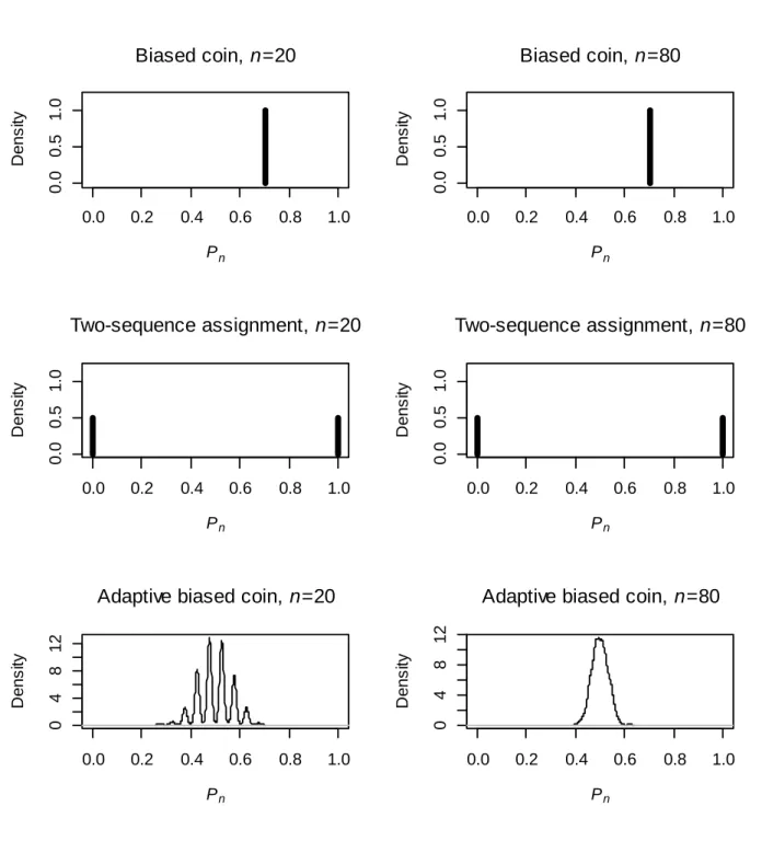
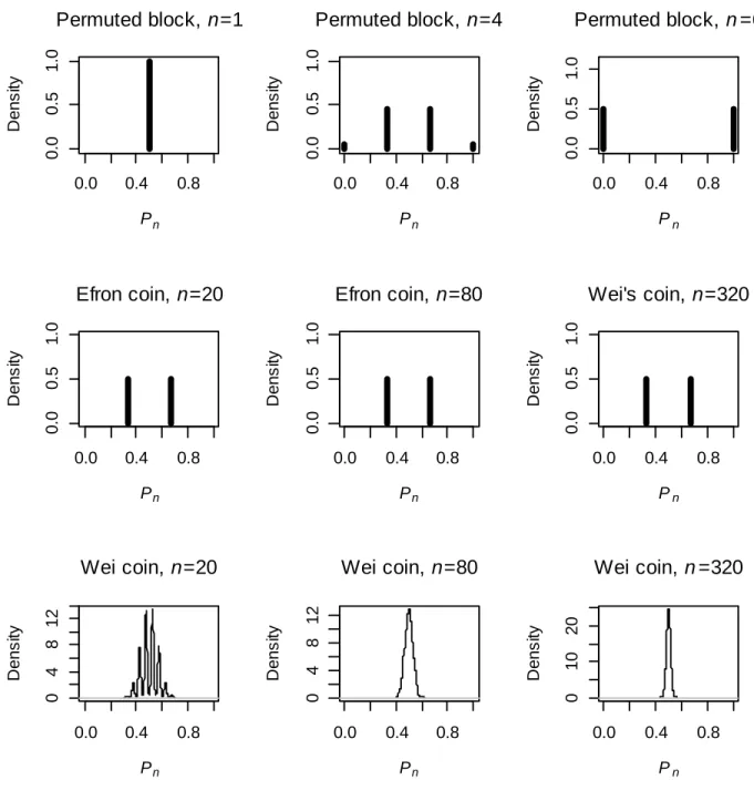
Figure 3.1. Density of Pn for designs... . 60
Figure 3.2. Density of Pn for designs in Section 4 with fixed target allocation... 61
Figure 3.3. Density of Pn for response adaptive designs from Section 4... 62
CHAPTER 1: INTRODUCTION AND LITERATURE REVIEW
The clinical trial has long history in biostatistics. One of the most important issues in clinical trials is how to assign patients to different treatments. One of the first ways proposed to do this is simple randomization. This method involves flipping a coin with a certain success probability and assigning patients to one of two treatments depending on the result of the coin flip. The problem with this approach is that it can lead to imbalances in the number of patients assigned to each treatment that can affect power. One way statisticians have sought to deal with this issue is to create more complex treatment assignment regimes that depended on the trial assignments previous to the current patient. There are many attractive features of such schemes, but one major drawback is that they introduce the possibility for new kinds of bias to enter the trial.
showed that this Bayesian design, which minimizes the Bayes risk of the experimenter’s strategy. However, this result depended on the simplicity of the two level distribution of bias known to the investigator.
Efron suggested an allocation scheme that involved flipping a fair coin if the allocation to each treatment was equal, and flipping a bias coin with bias towards the less frequent treatment if there was imbalance (Efron, 1971). In this scheme, the number of patients in the trial was unbounded. He referred to covariate bias as accidental bias. This is the bias that results from random differences in covariate values in the patient population. Selection bias, which is also important, is defined as the bias that results from the baseline characteristics of the patients assigned to each treatment differing due to knowledge that the investigator has about the previous patients or (Blackwell and Hodges, 1957).
Efron also introduced an early method to replace the coin flip as a treatment allocation scheme. It is called Efron’s coin (Efron, 1971). The idea is that if the number of patients assigned to each treatment is equal then a fair coin is flipped to determine the next treatment assignment; if there is an imbalance, then a biased coin with probability p > 0.5 is flipped, and if the coin lands heads, then the next patient is selected to decrease the imbalance. The value of p may vary. Efron mentioned that the “best” guessing strategy at patient n, if the treatments were unmasked and the goal is to guess the next treatment assignment, was to guess the treatment that appeared least often (Efron, 1971). This yielded an asymptotic probability of correctly guessing
the next treatment as 0.5+(r-1)/4r, which implies excess selection bias of (r-1)/4r. Here
Accidental bias is quantified as being , where is the covariance matrix of the treatment vector and z is the covariate vector (Efron, 1971). Recently a compact form for this matrix was discovered (Markaryan and Rosenberger, 2010). This bias must be less than the maximum eigenvalue of Efron, 1971), and the upper bound was recently sharpened (Markaryan and Rosenberger, 2010).
The doubly adaptive biased coin chooses the next treatment with probability:
( / )
( , ) ,
( / ) (1 ) (1 ) /(1 ) (0, ) 1,
(1, ) 0.
x g x
x x
g g
Where is the estimated target allocation for treatment 1, x is the actual target allocation for treatment 1, and is a nonnegative randomization parameter that is constant throughout the trial (Hu and Zhang, 2004).
Hu and Zhang show a law of the iterated logarithm of the doubly adaptive biased coin designs as well as several other designs (Wei, 1978). A law of the iterated logarithm is a standardization of the sum of a sequence of random variables that converges in probability but not almost surely. By using martingale methods and the law of the iterated logarithm, they prove asymptotic normality of allocation proportions under some general conditions. This law is used to show asymptotic normality of the allocation proportion of the doubly adaptive biased coin (Hu and Zhang, 2004). Joint bivariate normality of the allocation proportion and target allocation are also shown upon standardization by . The values in the covariance matrix for the multivariate normal distribution are determined by the same methods.
The doubly adaptive biased coin can be used for either continuous or binary outcomes. The variance of the allocation proportion for the doubly adaptive biased coin is smaller than that for the randomized play the winner rule, especially when the allocation proportion is close to 0.5 (Hu and Zhang, 2004).
1) g(v, v) = v and g(x, y) - g(x, v) --> 0 as y -> v when x and y represent discrete densities
2) gk(x,v) is Lipschitz continuous with an upper bound of 1 when x is a discrete density and xk is
greater than vk.
3) For any and each k in (1, ..., K), there exists a constant > 0 such that for all x, y with x1'= 1, y1'= 1, ,
> uniformly in x, y
with x1'= 1, y1'= 1, .
It is important to understand that condition 3 exists to avoid experimental bias. If all estimated target allocations for each of the k arms are not small, but the actual allocation to treatment k is very small, the probability of assigning the next treatment to k should not be too small in order to avoid large experimental bias. The authors claim that if the greater than sign is replaced by a less than sign then condition 3 follows from condition 2 (Hu and Zhang, 2004).
If the Lipschitz continuity constant referred to in the conditions for the randomization function is less than 0.5, then the convergence of the actual allocation proportion to the vector of target allocation proportions is of order and the convergence of the estimated target allocation vector is also of order Both of these convergences are almost sure.
Another design that was proposed after the doubly adaptive biased coin was the efficient randomized adaptive design (ERADE). This is design is a combination of Efron’s coin and the doubly adaptive biased coin. Let x be the actual allocation to treatment #1 in the trial, be the estimated target allocation, and be a parameter between zero and one. The ERADE assigns the next patient to treatment #1 with probability:
if x > ,
if x = ,
if x < .
When the log odds ratio, log
p q1 2/(q p1 2)
, is of interest, the allocation to treatment #1 that minimizes the asymptotic variance of the log odds ratio estimate is1 p q2 2 /( p q1 1 p q2 2)
(Ivanova, 2003). This allocation also minimizes the sample size
required to achieve given power if testing is based on the log odds ratio. The allocation that minimizes the expected number of failures for a fixed variance of the estimated odds ratio is
2 p2 / p1 p2
. The allocation that yields the same power as equal allocation for
testing the log odds ratio is 3 p q2 2/(p q1 1p q2 2). When min(p q1, 1)min(p q2, 2)
1 3
0.5 and any allocation inside the interval [0.5,3] yields higher or the same power for testing the log odds ratio. Similarly, when min(p q1, 1)min(p q2, 2) 310.5 and any allocation inside [3,0.5] yields higher or the same power than equal allocation. It happens that
1
i i
The Neyman allocation, 1= p q1 1 / ( p q1 1 p q2 2), maximizes the power of treatment comparison under a Z test for a when the sample size is fixed. It assigns more patients to the treatment with the larger variance, while the allocation 1 does the opposite. Therefore, the allocation 1 is “ethical” (assigns more patients to the better treatment) when, for example, both treatments have success rates below 0.5. Let without loss of generality p1 p2. When
1 2
0.5 p p any allocation inside the interval [0.5,3] is a desirable allocation for testing H0:
1 2 0
p p as it yields higher or the same power and assigns more patients to the better treatment than equal allocation. The allocation 1 is “ethical” when both treatments have success rates higher than 0.5. It has been argued that response adaptive designs are most useful in trials with highly successful treatments (Ivanova and Rosenberger, 2001). Also in trials where it is most desirable to minimize the number of treatment failures, the treatment failure as often death; therefore we discuss the case of comparing treatments with p1 p2 0.5 in more detail. For
1 2 0.5
p p any allocation inside the interval [0.5,3] is a desirable allocation for testing the log odds ratio as it yields higher or the same power and assigns more patients to the better treatment than equal allocation.
Historically, designing an allocation scheme for a clinical trial requires balancing a number of different factors. This includes the desire to assign patients to treatment that appears superior during the course of the trial, as well as to achieve higher power with such allocations as the Neyman allocation.
the Neyman allocation. The authors show that the allocation to treatment #1 converges almost surely to the target allocation as well under this scheme.
Some take the view that randomization not only mitigates biases but is the basis for inference, and is therefore very important (Rosenberger and Lachin, 1993). The first approach, however, introduces positive correlation between the sequential treatment allocations, which can increase the variance of the allocation proportion and therefore decrease power.
The Z test setup can be used to show that the size of the noncentrality parameter for the associated Chi squared distribution in the test corresponds to the power of the trial (Hu and Rosenberger, 2003). The authors use a power series expansion to show that the Neyman allocation maximizes this power. There are more complicated procedures that do as well, but what is necessary for these procedures to work is that the allocation proportion converge almost surely to constant.
These results are also generalized to a multi-treatment clinical trial setting where the test is an omnibus test of whether any are different from the null. The authors also use simulations to show that the urn allocation has the smallest failure rate and noncentrality parameter, a second design (with allocation probability proportional to ), has the next smallest of each, followed by the Neyman allocation with the highest power and highest failure rate.
derivatives of the target allocation by the inverse of the Fisher information when the target allocation is achieved. Besides Ivanova’s drop the loser design, Zelen’s play the winner rule also achieves this lower bound (Hu, Rosenberger and Zhang, 2006). In the proof of the main result a sequence of independent random variables is created from the original sequence via an application of the Martingale central limit theorem.
Some of the earliest statistical theory deals with trying to detect a linear relationship between a pair of random variables. However, often other relationships are of interest. Other attempts to capture these relationships statistically include CorGC (Delicado and Smrekar, 2009), mutual information (Breiman, 1968), and the Spearman rank correlation coefficient (Breiman, 1968). Mutual information is a way of assessing how close the relationship between two random variables is to independence. It is computed by taking the Kullback-Leibler divergence between the joint density and the product of the marginal densities. The Spearman correlation coefficient is based on the ranks of the data and is geared toward discovering a monotonic relationship. The CorGC is based on principal curves that are fit to the data. As with any two methods, the principal curve has drawbacks. The latter two methods make some assumptions about the relationship in the first place, while mutual information is harder to implement in smaller samples when the form of the density must itself be estimated.
In the middle of the last century (Renyi, 1959) several axioms were proposed that a measure of dependence between two random variables defined on the same probability space must have.
i) The measure should be defined for any pair of random variables (X,Y), neither of them being constant with probability 1.
iii) It should lie within [0,1]
iv) It should equal zero only in the case of independence.
v) It should equal one only in the case of strict dependence of the two random variables. vi) It should be invariant under functions of it two arguments that map the real line in a
one to one way onto itself.
vii) If the joint distribution is bivariate normal, then the function should be equal to the absolute value of the correlation coefficient.
Later in the twentieth century several different dependence measures were proposed,, but not all of them satisfied these axioms. The CorGC satisfied axioms ii), iii), and vii), as well as curved based analogues of axioms i) and v) (Delicado and Smrekar, 2009). The method is best designed for arguments distributed along a curve with no noise. Local measures of linearity on the curve are defined and then they are aggregated to obtain global measures of dependence.
the Pearson correlation, the comparison would indicate the strength of the linear relationship. Another potential drawback to this method is that it does not reveal the actual nature of the relationship, just that one exists.
It has also been shown on the machine learning side, that Reproducing Kernel Hilbert Space measures can be viewed as an extension of the distance covariance.
Another method to search for patterns in large data sets that was recently introduced is called the MINE statistic (Reshef, et al. 2011). This statistic also has the ability to detect arbitrary relationships in data sets. Like the Brownian distance covariance, it is invariant under affine transformations. It is also a rank statistic and it is this property that is used for computing tables of p values. The authors compare the statistic to several other statistics used to find general relationships, including the Brownian Distance Covariance. They note that it is only their statistic that has the property of equitability between different relationships with the same amount of noise. What they mean by this is that if two data sets are generated by drawing values from two different mathematical functions at random and perturbing each of them with the same amount of symmetric normal noise, then the value of the MINE statistic will be very similar for these two data sets. The statistic relies on the concepts of mutual information mentioned earlier. It statistic can be computed in a series of steps.
for the grid, given its dimensions. This maximum can be easily derived from the theoretical formula for mutual information. The maximum of this ratio across all grids that are investigated is called the MIC. A MINE statistic is a statistic that’s based on the MIC. These include ways to assess degrees of monotonicity or closeness to being a function. A larger MIC indicates a stronger relationship, and the grid that is retained from the calculation offer insight into what the explicit relationship is, which the Brownian distance covariance does not.
The MIC has certain desirable properties. First, in the case of statistical independence, it converges to zero in probability. Second, in the case of statistical dependence the statistic is bounded away from zero almost surely. Third, if the data are drawn from a noiseless functional relationship then the MIC converges to one. A property noticeably missing from this list is consistency: the authors do not show that the MIC converges to a number between zero and one in the case of noisy dependence. The Brownian Distance Covariance statistic, however, does have the property that it converges to its theoretical value in large samples. It has also been argued that the MINE statistic suffers from low power when the sample size is reasonable (200-300) (Gorfine-Orgad, 2012). Kosorok (personal communication) also observed that the MINE can register sizable correlations for random noise in reasonable samples, suggesting that Type 1 error may also be a problem in those samples as well. The MINE statistic is also not precisely equitable; it is a property that is established through simulation studies that are compare MINE to other methods.
can be said of the marginal variance. In survival analysis these questions are often more of interest than simply whether a relationship exists.
REFERENCES
Blackwell, D. and Hodges, J. L. (1957). Design for the control of selection bias. Annals of Mathematical Statistics. 28, 449-460.
Breiman, L. (1968). Probability. Boston: Addison-Wesley.
Delicado, P. and Smrekar, M. (2009). Measuring non-linear dependence for two random variables distributed along a curve. Statistics and Computing. 19, 255-269.
Efron, B. (1971). Forcing a sequential experiment to be balanced. Biometrika. 58, 403-417. Gorfine-Orgad, M. (2012).http://comments.sciencemag.org/content/10.1126/science.1205438 Hu, F. and Rosenberger, W.F. (2006). The Theory of Response-Adaptive Randomization in
Clinical Trials. New York: Wiley.
Hu, F. and Zhang, L.X. (2004). Asymptotic properties of doubly adaptive biased coin designs for multitreatment clinical trials. Annals of Statistics.32, 268-301.
Ivanova, A. (2003). A play-the-winner type design with reduced variability. Metrika. 58, 1-13. Ivanova, A. and Rosenberger, W.F. (2001). Adaptive designs for clinical trials with highly
successful treatments. Drug Information Journal.35, 1087-1093.
Markaryan, T. and Rosenberger, W.F. (2010). Exact properties of Efron’s biased coin randomization procedure. Annals of Statistics.38, 1546-1567.
Melfi, V.F., Page, C. and Geraldes, M. (2001). An adaptive randomized design with application to estimation. Canadian Journal of Statistics. 29, 107-116.
Renyi, A. (1959). On measures of dependence. Acta Mathematica Hungarica. 10, 441-451. Reshef, D.N., Reshef, Y.A., Finucane, H.K., Grossman, S.R., McVean, G., Turnbaugh, P.J.,
Lander, E.S., Mitzenmacher, M. and Sabeti, P.C. (2011). Detecting novel associations in large data sets. Science.33, 1518-1524.
Rosenberger, W. and Lachin, J. (1993). The use of response-adaptive designs in clinical trials.
Controlled Clinical Trials.14, 471-484.
Szekely, G.J. and Rizzo, M.L. (2009). Brownian distance covariance. Annals of Applied Statistics.3, 1236-1265.
Stigler, S. M. (1969). The use of random allocation for the control of selection bias. Biometrika. 56, 553-560.
Wei, L.J. and Durham, S. (1978). The randomized play-the-winner rule in medical trials. Journal of the American Statistical Association. 73, 840–843.
CHAPTER 2: HIGHER ORDER RESPONSE ADAPTIVE URN DESIGNS FOR HIGHLY SUCCESSFUL TREATMENTS
2.1 Introduction
desired allocation including the allocation that maximizes power.
An important metric of any allocation procedure is the amount of randomness it provides. In a deterministic procedure the next assignment can be predicted for sure if all previous
assignments and outcomes, in case of response adaptive allocation, are known. On the other side of a spectrum is a fully randomized allocation procedure, an allocation via a fair coin, in case of equal allocation, or biased coin otherwise. We use entropy to measure randomness of the designs, a measure that has not been used before when response adaptive designs were compared. This allows making a fair comparison of adaptive procedures since deterministic procedures are more efficient in targeting the desired allocation.
Hu and Rosenberger (2003) showed that the power of treatment comparison is closely related to the variability of the allocation proportion: the higher the variability the lower the power. The variability of the allocation proportion depends on the type of allocation procedure as well as on the allocation that the design targets and the amount of randomness it provides. The urn design of Ivanova (2003) yields the lowest variability as it achieves the lower bound of the asymptotic variance of the allocation proportion (Rosenberger and Hu, 2003; Hu, Rosenberger and Zhang, 2006), so does the ERADE (Hu, Zhang and He, 2009). The doubly adaptive coin design achieves the lower bound only when the procedure is deterministic (Rosenberger and Hu, 2003).
immigrated urn models. In this paper, we generalize the design of Ivanova (2003) in a different way by allowing the change in the urn composition to depend on several previous outcomes, not only the most recent outcome. This new generalization allows targeting a large spectrum of allocation proportions, including allocations that yield good power of treatment comparison. Since the design of Ivanova (2003) yields the lowest variability of the allocation proportion the new design has low variability as well and as the result has better power than competitors. The generalization, however, creates challenges in obtaining theoretical properties of the design since the new design can no longer be embedded into a family of stochastic processes unless
multidimensional state space is considered.
ratios or relative risk the power is maximized when more patients are assigned to the better treatment (Dette, 2004).
In this paper in Section 2 we review possible target allocations for trials comparing two treatments. We introduce higher order urn designs in Section 3. We present the theoretical result for normally distributed outcomes in Section 4. Simulations results are described in Section 5. In Section 6 we re-design the CALISTO trial. Section 7 is a discussion section.
2.2. Optimal allocations
Consider the case where two treatments are compared. Let Ni(n) be the number of subjects
assigned to treatment i, i = 1, 2, by the time a total of n subjects have been assigned, 1( ) 2( )
N n N n n. The allocation proportion to treatment 1 by the time n patients have been assigned is N n1( ) /n. The optimal allocation proportion can be determined by using multiple-objective optimality criteria (see Jennison and Turnbull, 2000, for more details). If treatment outcomes are binary from Bernoulli p( i), 0 pi 1, qi 1 pi, i = 1, 2, the allocation proportion on treatment 1, 1 p q1 1/( p q1 1 p q2 2), Neyman allocation, minimizes the variance of
1 2
ˆ ˆ
p p . Alternatively, it minimizes the total sample size required to achieve given power if the Wald’s test statistic is used to test H0: p1p2 0. The allocation that minimizes the expected number of failures for a fixed variance of the estimate of the parameter of interest or for fixed power (Rosenberger et al., 2001) is 2 p1/( p1 p2). Another allocation to mention is
3 p q1 1/(p q1 1 p q2 2)
; it yields the same power as equal allocation (see discussion of 3 in
the three corresponding allocations are 1 p q2 2 /( p q1 1 p q2 2),
2 p q2 2 / p q1 1 p q2 2
, and 3 p q2 2 / (p q1 1 p q2 2).
compared to equal allocation. Therefore 3 is an ideal target allocation in trials with highly successful treatments.
2.3. Higher order urn designs for binary outcomes
2.3.1. The second order urn design for binary outcomes
We introduce the second order urn design to create an urn design that focuses on variability of the estimated treatment effect rather than the mean. As a result the new design targets allocation proportions that are optimal or nearly optimal in terms of power, such as allocation 3. Also, by modifying a low variability design from Ivanova (2003), we obtain another low variability design and therefore we expect the new design to have good power compared to competitors as variability affects power negatively (Hu and Rosenberger 2003).. The design is defined as follows:
Second order urn design. The urn contains balls of three types. Balls of types 1 and 2 represent the two treatments. Balls of type 0 are called immigration balls. Initially the urn contains 2b + a balls; b balls of each treatment type and a, a > 0, immigration balls. Assume that
j patients have been treated so far, with at least one patient assigned to each treatment. If the jth patient was assigned to treatment i, let ( )
( )
i
i N j
X be this patient’s outcome. A ball is drawn from the urn at random. If the ball is of type 0, i.e., an immigration ball, no subjects are assigned to treatment, and the ball is returned to the urn together with 2 additional balls, one of each treatment type. If a ball corresponding to treatment i is drawn, i = 1, 2, the next subject is assigned to treatment i and an outcome ( )i( )
i N j
X is observed. If ( )i( ) ( )i( ) 1
i i
N j N j
the outcome of the previous subject assigned to treatment i, the ball is not returned. Otherwise, the ball is returned to the urn.
In the urn design of Ivanova (2003) the ball is not returned to the urn if there is a failure on the corresponding treatment. In the second order urn design the ball is not returned to the urn if the two most recent responses on the treatment are different, thus changing the urn composition according to the variability rather than the actual outcome. In this urn design the ball is not returned if outcomes are different, which increases the allocation to the treatment with smaller variance.
2.3.2. Limiting allocation proportion and variability of the second order urn design
When a response adaptive design is investigated, what is most important is the distribution of the proportion of patients assigned to each treatment, specifically the limiting distribution as the number of patients tends to infinity. To obtain this distribution for the second order urn design, we use the technique of embedding the design into a family of continuous time stochastic processes (Ivanova, 2003; Ivanova, 2006). First, we note that the design can be described by using the notion of continuous time (see Ivanova, 2003 and Ivanova, 2006, for more details), which is a useful mathematical construct not related to the real time in the medical experiment. Let Zi(t) be the number of balls of type i at time t, Ui(t) be the number of draws of a ball of type i
followed by a success on treatment i, and Yi(t) be the number of draws of a ball of type i
followed by a failure on treatment i, so that the number of trials on the ith treatment, i = 1, 2, is
Ni(t) = Ui(t) + Yi(t). Let I(t), the common immigration process, be the number of draws of balls of
type 0, immigration balls. By construction Zi(t) = Zi(0) + I(t) - Yi(t). The number of trials Ni(t) is
what interests us most, and the number of balls in the urn, Zi(t), is the quantity that defines this
et al. (2000) extended the technique from Cox and Miller (1965, p. 265) to obtain the differential equation for the joint probability generating functions. To describe the behavior of Ni(t), we will
obtain its joint generating function with the number of balls in the urn, Zi(t),
( ) ( )
( )
( , , ) Z ti N ti
i
G t z w E z w . Since the two most recent responses are used, consider the
generating function G0( )i ( , , )t z w describing the behavior of the process corresponding to treatment i when the preceding state was 0, the penultimate on treatment i was a success, and the generating function G1( )i ( , , )t z w describing the behavior of the process when the preceding state is 1, the penultimate response on treatment i was a failure, with
( ) ( ) ( )
0 1
( , , ) ( , , ) ( , , )
i i i
G t z w G t z w G t z w . Using backward equations, the following system of equations is obtained (see Appendix I for more details):
( ) ( ) ( )
( )
0 0 1
0
( ) ( ) ( )
( )
1 1 0
1
( , , ) ( , , ) ( , , )
( ) ( 1) ( , , )
( , , ) ( , , ) ( , , )
( ) ( 1) ( , , )
i i i
i
i i
i i i
i
i i
G t z w G t z w G t z w
q wz z q w a z G t z w
t z z
G t z w G t z w G t z w
p wz z p w a z G t z w
t z z
. (1)
Initial and boundary conditions are ( )
0 (0, , ) i
i
G z w q z, G1( )i (0, , )z w p zi , and G( )i ( ,1,1)t 1, i = 1, 2, with t 0, |z| 1, and |w| 1.
We are interested in the limiting allocation proportion for the urn p limn
N ni( ) /n
, where plim denotes convergence in probability. Ivanova (2003) showed that the limiting proportion can be computed by first obtaining
( )
1
log ( ,1, ) lim ( ) lim
i
t i t
w
G t w E N t
It might not be possible to obtain the closed form solution of the system of equations (1) except for special cases, however limtE N t t( i( ) / ) can be obtained by taking logs and then differentiating functions in the equations (1). We get limtE N t( i( ) / )t a/ (2p qi i). Using Theorems 3.1 and 3.2 from Ivanova (2000),
1 1 2 21
1 1 2 2 1 1 2 2 / (2 )
p lim ( ) /
/ (2 ) / (2 ) n
a p q p q
N n n
a p q a p q p q p q
,
which is 3.
The variability can be assessed by computing
1 2
( )
1
(1,2)
1 2 1 2
1 2 1
log ( ,1, )
( ) ,
( ), ( ) log ( ,1, , ) ,
i
i
w
w w
d G t w d
var N t w
dw dw
cov N t N t G t w w
w w
where G(1,2)( ,1,t w w1, 2) is a joint function for N1(t) and N2(t) (see Ivanova, 2006, for details). It
was not possible to obtain the closed form expressions forvar N t
1( )
, var N t
2( )
and
1( ), 2( )
cov N t N t for given t and as t so we resorted to numerical computations.
2.3.3. Higher order urn designs for binary outcomes
To describe this extension we first note that the second order design defined in Sect ion 3.1 can be alternatively defined using the estimate of success probability obtained from the two most recent observations. The estimate
( ) ( )
( ) ( ) 1
ˆ / 2
i i
i i
i N j N j
p X X , i =1, 2, can take on three
possible values 0, 1/2 and 1. The ball of type i is not returned if ˆpi0.5. Similarly, in the kth order urn design, the estimate of success rate is based on the k most recent responses:
( ) ( ) 1 1
ˆ /
i
k i
i m N j m
p
X k. Let an integer be such that k2, if k is even, or k 21, if k is odd. Consider the kth order design where the ball is not returned if ˆpi /k or ˆpi 1 /k, that is, the ball is not returned if the estimate of success rate is the closest possible to 0.5. The probability of not returning the ball is ki i i
Q C p q if k2, or k 1 k 1
i i i i i
Q C p q C p q
( )
k k
i i i i i i
C p q p q C p q if k21. Here k
C k!/
!(k)!
is a binomial coefficient with 0k
C , if < 0 or > k. The limiting allocation proportion for this urn design (Ivanova, 2003) is equal to Q2/(Q1Q2) p q2 2 /(p q1 1 p q2 2) ( )
. For example, when k = 3 the limiting allocation proportion is (1) p q2 2/ (p q1 1p q2 2)3, when k = 4, the allocation is
2 2 2 2 2 2
2 2 1 1 2 2
(2) p q /(p q p q )
. For p1 p2 and , ( ) ( ), therefore for all > 1 ( ) is
closer to 1 than (1)3. Allocations ( ) for > 1 might be desirable for trials with the goal of selecting the best treatment, however, as was discussed in Section 2, the power under allocations ( ) with > 1 is lower than under 3 or under equal allocation.
With the use of a biased coin the kth order urn design can be made to target the desirable allocation 3. Consider a kth order urn design, k = 4, 5…, where the ball is not returned if
ˆ /
2 2
1 / 1
k k k k
m m
C C C C lands heads. To compute the limiting allocation proportion for this design we first compute the probability of not returning the ball
2
1 1
2 1 1
1
1
2 2
1 1 1 1
2
2 ' 2 ' 2
2 2 2
0
1 1 1
( ) .
k k k
k k
k m k m k m k m
m
i k k m i i k i i m i i
m m m
k k k k
k m k m k
i i m i i i i i i i i
k k k
m
C C C
Q C p q p q C p q
C C C
C C C
p q C p q p q p q p q
C C C
Therefore the limiting allocation is equal to Q2/(Q1Q2) p q2 2/(p q1 1p q2 2)3. For example, when k = 4, the possible values for ˆpi are 0, 1/4, 1/2, 3/4, and 1. According to the design described above, the ball is not returned if ˆpi1/ 2; or if ˆpi 1 / 4,3 / 4 and a biased coin with the probability of heads equal to 3/4 lands heads. When k = 5, the ball is not returned if
ˆi 2 / 5,3 / 5
p ; or if ˆpi1 / 5,4 / 5 and a biased coin with the probability of heads equal to 2/3 lands heads.
2.4. Higher order urn designs for normally distributed outcomes
In this section we define the kth order urn design for continuous outcomes and prove a result about its limiting allocation. As response adaptive designs are mostly advantageous when treatments with binary outcomes are compared (unless the variances of continuous responses in the two arms are very different), the goal of this section is to provide insights into how to construct higher order urn designs for binary outcomes that yield good power of treatment comparison.
1 2
ˆ ˆ
is the Neyman allocation Ney 1/( 1 2). Assume that outcomes of treatment i
come from 2
( ,i i )
N and let ˆ2 i
be the estimate of the variance based on the k most recent observations on treatment i, defined as
22 ( ) ( )
( ) 1 ( ) 1
1 1
ˆ /( 1), where / .
i i
k k
i i
i N j m N j m
m m
X X k X X k
Then, the ball is not returned to the urn if ˆ2 i
for some . The following theorem characterizes the limiting distribution.
Theorem. As , the limiting allocation proportion for the kth order urn design, k 1, with normally distributed outcomes tends to 1/( 1 2).
Proof. The distribution of (k1) ˆi2/ i2 is chi-squared with degrees of freedom df k 1. Let F
be the cumulative distribution function of chi-squared distribution with df k 1, and f be its density function. The probability of not returning the ball is F
(k1) / i2
and the limiting proportion is (Ivanova, 2003)
2 1 1 2 2 0 1 2( 1) / ( )
plim lim
( 1) / ( 1) /
n
F k
N n
n F k F k
.
Now it follows from L’Hôpital’s Rule that:
2 2 2
1 1 1 2
2 2 2 2
2 2
0 0
1 1 2 2 1 2
1 2
( 1) / ( / ) /
lim lim
( / ) / ( / ) /
( 1) / ( 1) /
F k f
f f
F k F k
,
since f x( )xk/ 2 1ex/ 2.
basis to the general strategy of constructing higher order urn designs for binary outcomes described in previous sections.
2.5. Comparison with competing designs
In this section we compare the new urn designs with the doubly adaptive biased coin design (Hu and Zhang, 2004) and the efficient randomized adaptive design (Hu, Zhang and He, 2009).
The doubly adaptive biased coin design (Hu and Zhang 2004) allocates patient j to treatment i with probability g N j( i( ) /(j1), )ˆ , where
ˆ is the target proportion estimated from the data. We use the choice of g from Hu and Zhang (2004):
( / )
( , ) ,
( / ) (1 ) (1 ) /(1 ) (0, ) 1,
(1, ) 0.
x g x x x g g
Here is a design parameter controlling the amount of randomization in the design. Let
1 2 (p p, )
be the target allocation proportion as a function of p1 and p2, for example,
1 2 2 2 1 1 2 2 ( ,p p ) p q / p q p q
for inverse Neyman allocation. Hu and Zhang (2004) give
the following formula for the asymptotic variance, 2, of N n1( ) /n
2
2 1 2
2
2
1 1 2 1 2
2 2
2 1 2 1 1 1 2 2 2
2
1 1 2 2 1 2
2 1
, where 1 2 1 2
( , ) 1 ( , ) and
( , ) ( , )
.
( , ) 1 ( , )
p p p p
p p p q p p p q
p p p p p p
When 0, the design is fully randomized, and the variance is 12222; when the design is deterministic, the variance is 22 and is equal to the lower bound of the asymptotic variance. Hu and Rosenberger (2005) recommended using the design with 2.
The ERADE (Hu, Zhang and He, 2009) is a generalization of Efron’s coin which attains the lower bound of the asymptotic variance and can target any desirable allocation. The ERADE requires specifying a design parameter π, 0 1, that reflects the degree of randomization, with larger values of π corresponding to more randomization and variability. The design is defined as follows. As before,
ˆ is the estimated target allocation for treatment 1. Then the next patient is assigned to treatment 1 with probability
ˆ if the actual allocation to treatment 1 exceeds
ˆ; with probability
ˆ if the two estimated allocations are equal; with probabilityˆ
1 (1
) if the actual allocation exceeds the estimated target allocation. Hu, Zhang and He (2009) studied the choice π and found that the simulated results of π = 1/8 and 1/4 were very similar to the results of π = 1/2 in terms of allocation proportion and its variability, and the ERADE with π = 3/4 has a slightly larger variability than others. They recommended using π in [0.4, 0.7]. Since the ERADE with π = 0.5 performed very similar to lower values of ERADE we used the ERADE with π = 0.5.We compared designs based on variability of allocation proportion and randomness. Randomness was quantified by summing entropy of the allocation distribution for each
assignment, 1
log( ) N
j j
j
, where j is the probability of being assigned to treatment 1 after (j –1) patients have been assigned. For a given p1 and p2, the sample size, N, used for entropy
testing based on the log odds ratio. For the adaptively biased coin design j g N j( 1( ) /(j1), )ˆ . In the case of the third order urn design, j is equal to
1
1 1 2
0 0
( ( ) ) ( ( ) ( ) 1 2 )
m
m k
z j m z j z j k
, where z ji( ) is the number of balls of type j in theurn right after the most recent treatment (non-immigration) ball was chosen, and the sum is over the number of immigration balls m to be drawn before a treatment ball is drawn. The product in the denominator is the probability that m - 1 immigration balls are chosen before z ji( ) is finally chosen. We have not been able to obtain a closed form for the sum. Noting that that the sum of all terms after the mth term is less than the mth term (see Appendix II) it is easy to obtain the numerical value for the sum with any degree of accuracy. We computed the sum within 10-14 of the true value.
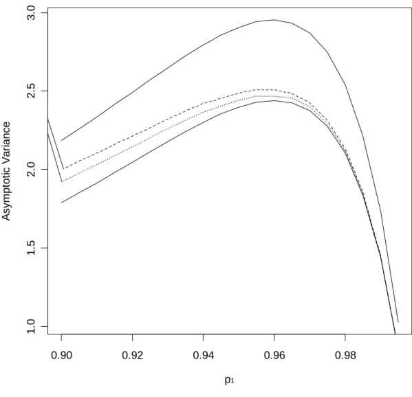
First, we compare the asymptotic variance of the second and third order urn designs with the lower bound of the asymptotic variance of designs that target 3 and the asymptotic variance of the doubly adaptive biased coin design with 2. Fig. 1 displays the asymptotic variances for p2 0.90 and p1 in [0.90, 0.99]. Even though the design from Ivanova (2003) achieves the lower bound of the asymptotic variance, the higher order urn designs do not, but their variances are very close to the lower bound and are significantly smaller than those of the biased coin design with 2.
Second, we compared the designs for sample sizes required to achieve 80% power for treatment comparison if equal allocation was used. We compared the second and third order urn designs to the adaptively biased coin design with 2 and ERADE with π = 0.5 for values of p1
randomness the designs provide. The regions of (p1, p2) sample space where the third order urn
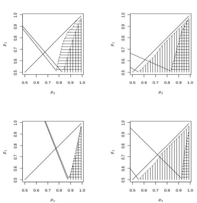
design has higher entropy, which is more desirable, are marked with vertical lines in Fig. 2. Elements of (p1,p2) space where the asymptotic variance for the third order urn design was
smaller marked with horizontal lines in Fig. 2. In Section 2 we proposed 3 as the target allocation in a trial where treatment comparison is based on log odds ratio. The first row of Fig. 2 shows the comparison with the adaptively biased coin design and the ERADE targeting 3, the second row targeting 1. Fig. 2 shows that the third order urn design performs well against the adaptively biased coin design and the ERADE targeting 3 in about half of the 2-dimensional region of (p1, p2). When the coin design and the ERADE target 1 the region where the new
design is better is smaller, however, the advantage of the proposed design still holds for trials where highly successful treatments are compared.
2.6. Example: re-designing CALISTO trial
power. Our proposed urn design targets 3 0.866, the allocation that yields the same power as equal allocation by less treatment failures. For the success probabilities in CALISTO trial both the coin design and the ERADE perform better when targeting 1, therefore we describe simulation results for these two designs for 1 target only. To redesign the CALISTO trial we first found the values of parameters in the coin design and π in the ERADE design that yield the same randomness, measured by the total entropy, as the third order urn design. These parameters were 0 for the coin design and π = 0.28 for the ERADE. Then trials with assignments by the coin design and the ERADE were simulated. Results are presented based on 5000 simulated trials. Simulation study was repeated with recommended values 2 and π = 0.5 yielding similar conclusions. To simulate CALISTO trial we resampled from CALISTO data knowing that 13 out of 1502 failures were observed in Arixtra arm and 88 out of 1500 in placebo arm. Results when data were simulated from Bernoulli distribution with success probabilities
1 0.991
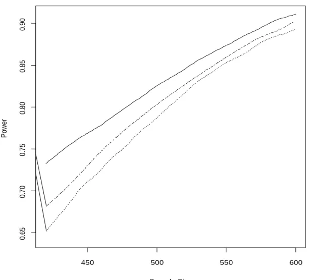
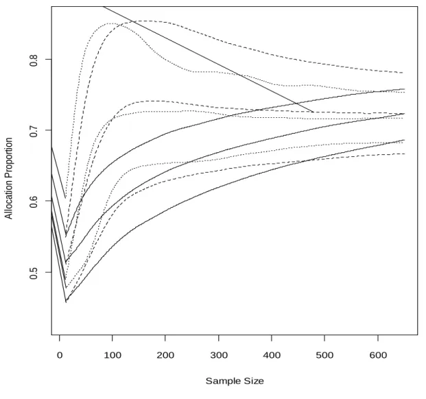
Fig. 3 shows power curves in the informative region of total sample sizes, between 300 and 600, for the third order urn design, the ERADE, and equal allocation. Power for the adaptively biased coin design is inferior and is not shown. As seen from Fig. 3, the proposed urn design has better power than equal allocation and the ERADE. Better power for the urn design is the result of low variability of the allocation proportion (Fig. 4). The average allocation proportion and its 25th and 75th percentiles (Fig. 4) show that the allocation proportion of the doubly adaptive coin design and the ERADE converges to the limiting proportion quickly, but that the variability of the allocation proportion is high. For example, for the total sample size of 300, the allocation proportion in 10% of the trials is 90:10 or more extreme when the target is, in fact, 1 0.717. This makes the design more sensitive to time trends and lower in power when multiple interim analyses are performed. Though the urn design converges slower, it is far less variable.
We also performed simulations with delayed response. As shown by Bai, Hu and Rosenberger (2002) the asymptotic properties of response adaptive designs under delay in outcome are the same as without a delay unless the delay is substantial and as long as adaptations are done frequently. We assumed that the data from the first patient was only available when the
performing better than the urn design. Note that if the adaptations of the allocation proportion are only performed once or twice during the trial, the proposed urn design is not suitable and the adaptively biased coin or the ERADE should be used. Both the coin design and the ERADE estimate the success probabilities using all available data and compute the desirable allocation proportion.
2.7. Conclusions
The doubly adaptively biased coin design and ERADE estimate the target allocation from the data and therefore can target any desired allocation proportion. Both designs converge rapidly to the target, however, the variability of the allocation proportion is high as well. The proposed higher order urn designs converge to the target allocation more slowly, however, are far less variable. In the example considered, the third order urn design does not result in extreme allocations and yields higher power than the doubly adaptive coin design, the ERADE and equal allocation. Another advantage of the proposed urn designs is that one does not have to know the most recent estimates of the treatments’ success probabilities p1 and p2. For the third order urn design, for example, one only needs to know if there were any failures among the most recent 3 responses. Therefore, if data used for a recent adaptation are revealed, an investigator will not know the most recent estimates of p1 and p2.
Figure 2.1. The asymptotic variance. Consider the second order urn design (dashed line), the third order urn design (dotted line) and the doubly adaptive biased coin design with parameters = 2 (upper solid line) and = (lower solid line). Success rate p2 = 0.9.
0.90 0.92 0.94 0.96 0.98
1
.0
1
.5
2
.0
2
.5
3
.0
p1
A
sym
p
to
ti
c
V
a
ri
a
n
Figure 2.2. Range of success probabilities p1 and p2. When third order urn design has smaller asymptotic variance (horizontal lines) and higher entropy (vertical lines) than the doubly adaptive coin design with = 2 (left panel) or ERADE with π = 0.5 (right panel). The diagonal line is the boundary of the sample space. The first row is for the coin design and ERADE targeting 3, the second for 1.
0.5 0.6 0.7 0.8 0.9 1.0
0. 5 0. 6 0. 7 0. 8 0. 9 1. 0 p2 p1
0.5 0.6 0.7 0.8 0.9 1.0
0. 5 0. 6 0. 7 0. 8 0. 9 1. 0 p2 p1
0.5 0.6 0.7 0.8 0.9 1.0
0. 5 0. 6 0. 7 0. 8 0. 9 1. 0 p2 p1
0.5 0.6 0.7 0.8 0.9 1.0
Figure 2.3. Power for the CALISTO trial. Consider p1 0.991 and p2 0.941 for third order urn design (solid line), the equal allocation (dotted-dashed line) and the ERADE with π = 0.28 targeting 1 (dotted line).
450 500 550 600
0
.6
5
0
.7
0
0
.7
5
0
.8
0
0
.8
5
0
.9
0
Sample Size
P
o
w
e
Figure 2.4. Allocation proportion and quantiles. The allocation proportion and its 25th and 75th percentiles for the trial with p10.991 and p2 0.941 for third order urn design (solid lines), the doubly adaptive coin design with = 2 (dashed lines), and ERADE with π = 0.5 (dotted lines) plotted against the sample size.
0 100 200 300 400 500 600
0
.5
0
.6
0
.7
0
.8
Sample Size
A
llo
ca
tio
n
P
ro
p
o
rt
io
REFERENCES
Athreya, K. B. and Karlin, S. (1968). Embedding of urn schemes into continuous time branching processes and related limit theorems. Annals of Mathematical Statistics 39,1801–1817. Bai, Z. D., Hu, F. F. and Rosenberger, W.F. (2002). Asymptotic properties of adaptive designs
for clinical trials with delayed response. Annals of Statistics30, 122-139.
Baldi Antognini, A. and Giovagnoli, A. (2010). Compound optimal allocation for individual and collective ethics in binary clinical trials. Biometrika97, 935-946.
Connor E. M., Sperling R. S., Gerber R., Kiselev, P., Scott, G., O'Sullivan, M. J., et al. (1994). Reduction of maternal-infant transmission of human immunodeficiency virus type 1 with zidovudine treatment. New England Journal of Medicine331, 1173-1180.
Cox, D. R. and Miller, H. D. (1965). The Theory of Stochastic Processes, New York: Wiley. Decousus, H., Prandoni, P., Mismetti, P., Bauersachs, R. M., Boda, Z., Brenner, B., Laporte, S.,
Matyas, L., Middeldorp, S., Sokurenko, G. and Leizorovicz, A. (2010). Fondaparinux for the treatment of superficial-vein thrombosis in the legs. New England Journal of Medicine 23(363), 1222-1232.
Holger, D. (2004). On robust and efficient designs for risk estimation in epidemiological studies.
Scandinavian Journal of Statistics31, 319-331.
Eisele, J. R. (1994). The doubly adaptive biased coin design for sequential clinical trials. Journal of Statistical Planning and Inference38, 249–261.
Hjalmarson, A. and the MIAMI Trial Steering Committee (1985). Metoprolol in acute myocardial infarction (MIAMI). A randomised placebo-controlled international trial.
European Heart Journal6(3), 199-226.
Hu, F. and Rosenberger, W. F. (2003). Optimality, variability, power: Evaluating response-adaptive randomization procedures for treatment comparisons. Journal of the American Statistical Association98, 671–678.
Hu, F. and Ivanova, A. (2004) Adaptive design. In Encyclopedia of Biopharmaceutical Statistics, Marcel Dekker, New York, 1-6.
Hu, F. and Rosenberger, W. F. (2006). The Theory of Response-Adaptive Randomization in Clinical Trials. New York: Wiley and Sons.
Hu, F., Rosenberger, W. F. and Zhang, L.-X. (2006). Asymptotically best response-adaptive randomization procedures. Journal of Statistical Planning and Inference 136, 1911–1922. Hu, F. and Zhang, Y. (2004). Asymptotic properties of doubly adaptive biased coin designs for
Hu, F., Zhang, Y. and He, X. (2009). Efficient randomized-adaptive designs. Annals of Statistics 37, 2543-2560. Ivanova, A. (2003). A Play-the-Winner-Type Urn Design with Reduced Variability. Metrika58, 1-13.
Ivanova, A. (2006). Urn designs with immigration: useful connection with continuous time stochastic processes. Journal of Statistical Planning and Inference 136, 1836-1844.
Ivanova, A., Rosenberger, W. F., Durham, S. D. and Flournoy, N. (2000). A birth and death urn for randomized clinical trials: Asymptotic methods. Sankhyā B 62,104–118.
Ivanova, A. and Rosenberger, W. F. (2001). Adaptive designs for clinical trials with highly successful treatments. Drug Information Journal35, 1087-1093.
Pocock S. J. (1977). Group sequential methods in the design and analysis of clinical trials.
Biometrika 64, 191-199.
Rosenberger, W. F., Stallard, N., Ivanova, A., Harper, C. and Ricks, M. (2001). Optimal adaptive designs for binary response trials. Biometrics57 (3), 833-837.
Simoons, M., Krzemiñska-Pakula, M., Alonso, A., Goodman, S., Kali, A., Loos, U., et al. (2002). Improved reperfusion and clinical outcome with enoxaparin as an adjunct to streptokinase thrombolysis in acute myocardial infarction. The AMI-SK study. European Heart Journal23, 1282-1290.
Tebbe, U., Michels, R., Adgey, J., Boland, J., Caspi, A., Charbonnier, B., et al. (1998). Randomized, double-blind study comparing saruplase with streptokinase therapy in acute myocardial infarction: the COMPASS Equivalence Trial. Journal of American College of Cardiology31, 487-493.
Wallentin, L., Bergstrand, L., Dellborg, M., Fellenius, C., Granger, C. B., Lindahl, B., et al. (2003). Low molecular weight heparin (dalteparin) compared to unfractionated heparin as an adjunct to rt-PA (alteplase) for improvement of coronary artery patency in acute myocardial infarction-the ASSENT Plus study. European Heart Journal24, 897-908.
Wei, L. J. and Durham, S. (1978). The randomized play-the-winner rule in medical trials.
Journal of the American Statistical Association 73, 840–843.
Zelen, M. (1969). Play the winner rule and the controlled clinical trial. Journal of the American Statistical Association 64, 131–146.
Zhang, Y., Hu, F., and Cheung, S. H. (2006). Asymptotic theorems of sequential estimation adjusted urn models. The Annals of Applied Probability16, 340-369.
CHAPTER 3: THE PROPERTIES OF ENTROPY AS A MEASURE OF RANDOMNESS IN THE CLINICAL TRIAL
3.1. Introduction
The interpretation of between-group comparisons in a clinical trial is facilitated by the creation of treatment groups that are similar to each other in baseline composition. Selection bias is a major impediment to baseline similarity of treatment groups especially in unmasked clinical trials. Selection bias occurs when expected responders are enrolled or denied enrollment based on the knowledge of treatment to be allocated next (Blackwell and Hodges, 1957), and how healthy the patients are. To minimize selection bias one needs to minimize predictability of future allocations based on past ones. One way to measure predictability is to define a reasonable guessing strategy and then compute the expected number of correctly predicted treatment assignments. Allocation procedures that minimize selection bias against various guessing strategies have been identified (Blackwell and Hodges, 1975; Stigler, 1969). One drawback to this approach is that it is somewhat arbitrary, because the expected value is just one measure of a distribution. Also, this requires assumptions about the distribution of healthiness in the patient population, which is generally difficult to evaluate. Finally, in a clinical trial where a response adaptive randomization design is used, it is not clear what the best guessing strategy for the investigator is, and thus it is not clear how to calculate bias.
assignments are known. This approach relies on information theory, specifically, Claude Shannon’s definition of entropy (Shannon 1959), which quantifies the amount of information observer has about the values a random variable may take. The greater the entropy, the less information the observer has. The formula for entropy of a discrete probability distribution taking on k values (which is the type of distribution the treatment assignment random variable will have) is
1
log( ) k
i i
i
p p
,where there are k different possible treatments, and pi is the probability of the ithtreatment being