ISSN: 1311-1728 (printed version); ISSN: 1314-8060 (on-line version)
doi:http://dx.doi.org/10.12732/ijam.v29i6.8
STUDY OF A ONE-DIMENSIONAL UNSTEADY GAS DYNAMIC PROBLEM BY ADOMIAN
DECOMPOSITION METHOD Manoj Singh1, Arvind Patel2§, Ruchi Bajargaan3
1,2,3 Department of Mathematics
University of Delhi 110007, Delhi, INDIA
Abstract: The system of gas dynamic equations governing the motion of one-dimensional unsteady adiabatic flow of a perfect gas in planer, cylindrical and spherical symmetry is solved successfully by applying the Adomian decom-position method under the exponential initial conditions. The solution of the system of equation is computed up to the five components of the decomposition series. The variation of the approximate velocity, density and pressure of the fluid motion with position and time is studied. It is found that there exists discontinuity or shock wave in the distribution of flow variables. The solution of system of gas dynamic equations by Adomian decomposition method is con-vergent for a domain of position and time. The decomposition method provides the variation of flow-variables with position and time separately which was not possible in similarity method.
AMS Subject Classification: 35L65, 76N15, 76M99
Key Words: system of gas dynamic equations, Adomian decomposition method, unsteady adiabatic flow
1. Introduction
The conservation laws for the motion of a gas in its mathematical formulation is written as a system of gas dynamic equations for mass, momentum and
energy. This system of gas dynamic equation is complemented by the equation of the state of the gas. The solution of the system of one-dimensional unsteady gas dynamic problem under the suitable initial condition is an important field of study. The solution of the system of gas dynamic equations are studied in literature and is solved by the different methods. One of the important and widely used method to solve the equations is similarity method but it needs the much computational work, knowledge of geometrical aspects of the problem and give solution in term of similarity variable, not in term of space and time variables directly, [1]. Recently, considerable amount of research work has been invested in applying the Adomian decomposition method to a wide class of linear and non-linear ordinary and partial differential equation as well as integral equation [2, 3, 4, 5, 6, 7, 8, 9, 10]. The Adomian decomposition method was introduced and developed by George Adomian [11]−[12] and is well addressed in the literature. This method has been used in the solution of scalar gas dynamic equation [13]−[14]. The system of gas dynamic equation has been solved by the Adomian decomposition method in two dimension for polytropic gas [15]. But the system of gas dynamic equations for the unsteady adiabatic flow of a perfect gas in one dimension for all the three type of symmetry namely planer, cylindrical and spherical has not been studied.
In the present work, we have solved the system of non-linear one-dimensional unsteady gas dynamic equations for adiabatic flow of a perfect gas in all the three symmetry under the variable initial condition by applying the Adomian decomposition method [12], [16] and [17]. The convergence and accuracy of the solution is discussed. The variation of flow-variables with position and time is presented which show that there exist a discontinuity or shock wave in the flow field. All the computations are performed usingMathematica 9.
2. Basic equations and initial conditions
The system of gas dynamic equations governing the motion of a one-dimensional unsteady adiabatic flow of a perfect gas in planer, cylindrical and spherical symmetry is given by [1]
∂u′ ∂t′ +u
′∂u ′
∂r′ + 1
ρ′
∂p′
∂r′ = 0, (1)
∂ρ′ ∂t′ +u
′∂ρ ′
∂r′ +ρ ′∂u
′
∂r′ + (ν−1)
ρ′u′
∂ ∂t′(
p′ ρ′γ) +u
′ ∂
∂r′(
p′
ρ′γ) = 0, (3)
whereu′,ρ′ andp′ are the velocity density and pressure respectively at position
r′ and time t′, γ is adiabatic exponent, ν is symmetry parameter which takes the values 1, 2 and 3 for the planer, cylindrical and spherical symmetry. The initial conditions for the motion is taken as
u′(r′,0) =u0e
−r′
l0 , ρ′(r′,0) =ρ
0e
−r′
l0 , p′(r′,0) =−ρ0u
2 0
3 e −3r′
l0 , (4)
where 0 ≤ r′ < ∞, t′ ≥ 0 and l0, u0 and ρ0 are dimensional constant. The
initial condition is consistent with the equation of motion (1). The equation of state for the perfect gas is p′ = ρ′RT where R and T are gas constant and temperature respectively. The technique to make the above equations dimensionless consists of introducing a simple change of variables t′ = t0t,
r′ =l0r,u
′
=u0u,ρ
′
=ρ0ρ and p
′
=ρ0u20p, where t
′
,r′,u′, ρ′ and p′ are the original dimensional variables,t,r,u,ρand pare corresponding dimensionless variables, and t0, l0, u0 and ρ0 are characteristic time, characteristic length,
characteristic velocity and characteristic density. Under the transformation the equations of motion of one-dimensional unsteady adiabatic flow of a perfect gas in planer, cylindrical and spherical symmetry reduces as
∂u ∂t +u
∂u
∂r +
1
ρ ∂p
∂r = 0, (5)
∂ρ ∂t +u
∂ρ ∂r +ρ
∂u
∂r + (ν−1) ρu
r = 0, (6)
∂ ∂t(
p ργ) +u
∂ ∂r(
p
ργ) = 0, (7)
and the initial conditions in non-dimensional form become
u(r,0) =e−r, ρ(r,0) =e−r, p(r,0) =−(1/3)e−3r, (8)
3. Basic idea of Adomian decomposition method
In Adomian decomposition method, we consider the partial differential equation in an operator form
Lu+Ru+N u=g, (9)
whereL is highest order linear operator which is assumed to be invertible and
R is linear operator of order less than order ofL,N is non-linear operator and
gis a source term. We apply the inverse operatorL−1to both sides of equation
(9) and using the given condition, we obtained
u=f −L−1(Ru)−L−1(N u), (10)
where the function f represents the terms arising from integrating the source term g and using the given condition, all are assumed to be prescribed. The standard Adomian decomposition method suggests the solution u in form of infinite series of the components, given by
u =
∞
X
n=0
un, (11)
whereun,n≥0 are components ofu. The non-linear operatorN is decomposed
in series form
N =
∞
X
n=0
An, (12)
whereAn are called Adomian polynomials. The aim of decomposition method
is to determine the componentsu0, u1, u2...; recursively and elegantly. The
Ado-mian polynomials can be generated for all form of non-linearity [18]−[19]. The Adomian polynomials Anare generated according to the algorithms previously
published in [19] and standard Adomian decomposition scheme introduced in [12]−[20]. On substituting Eq. (11) into Eq. (10) we get
∞
X
n=0
un=f−L−1(R
∞
X
n=0
un)−L−1(N
∞
X
n=0
un). (13)
Following the Adomian analysis in Eq. (13), the non-linear partial differential Eq. (9) with the condition is transformed into a set of recursive relations
u0 =f, (14)
uk+1=−L−1(Ruk)−L−1(N uk); k≥0. (15)
From Eqs. (14) and (15), by putting the componentsun,n≥0 in Eq. (11) the
4. Solution of the system of gas dynamic equations
Firstly we eliminate ∂ρ/∂tin Eq. (7) by using Eq. (6) then we write the basic Eqs. (5), (6) and (7) in the following operator form
Ltu+uLru+ (1/ρ)Lrp= 0, (16)
Ltρ+uLrρ+ρLru+ (ν−1)ρu/r= 0, (17)
Ltp+γpLru+uLrp+γ(ν−1)pu/r= 0, (18)
where Lt and Lr are the partial differential operators given byLt =∂/∂t and
Lr=∂/∂r. Then following the standard Adomian method, Eqs. (16)–(18) can
be written as
u(r, t) =e−r−L−t1(uur)−L−t1(pr/ρ), (19)
ρ(r, t) =e−r−Lt−1(uρr)−Lt−1(ρur)−(ν−1)L−t1(ρu/r), (20)
p(r, t) = −e −3r
3 −γL −1
t (pur)−L−t1(upr)−γ(ν−1)L−t1(pu/r). (21)
Let us assume the solution u, ρ and p of the Eqs. (16)–(18) in the form of decomposition series as
u(r, t) = ∞
X
n=0
un(r, t), (22)
ρ(r, t) = ∞
X
n=0
ρn(r, t), (23)
p(r, t) = ∞
X
n=0
pn(r, t). (24)
The non-linear term uur, pr/ρ, uρr, ρur, pur and upr in Eqs. (19)–(21) is
uρr=
∞
X
n=0
An, ρur =
∞
X
n=0
Bn, (25)
uur =
∞
X
n=0
Cn,
pr
ρ =
∞
X
n=0
Dn, (26)
pur =
∞
X
n=0
En, upr=
∞
X
n=0
Fn, (27)
whereAn,Bn,Cn,Dn,EnandFnare Adomian polynomials. Substituting Eqs.
(22)–(24) and (25)–(27) into both sides of Eqs. (19)–(21) we find
∞
X
n=0
un(r, t) =e−r−L−t1(
∞
X
n=0
Cn)−L−t1(
∞
X
n=0
Dn), (28)
∞
X
n=0
ρn(r, t) =e−r−L−t1(
∞
X
n=0
An)−L−t1(
∞
X
n=0
Bn)
−(ν−1)L−t1( ∞ X n=0 ρn ∞ X n=0
un)/r, (29)
∞
X
n=0
pn(r, t) =−e−3r/3−γL−t1(
∞
X
n=0
En)−L−t1(
∞
X
n=0
Fn)
−γ(ν−1)L−t1( ∞ X n=0 pn ∞ X n=0
un)/r. (30)
Following the decomposition method in Eqs. (28)–(30) we obtained the recur-sive relation for gas dynamic Eqs. (16)–(18) in an operator form as
u0(r, t) =e−r, (31)
u1(r, t) =−L−t1(C0)−L−t1(D0), (32)
ρ0(r, t) =e−r, (34)
ρ1(r, t) =−L−t1(A0)−L
−1
t (B0)−(ν−1)L
−1
t (p0u0/r), (35)
ρk+1(r, t) =−L−t1(Ak)−L−t1(Bk)−(ν−1)Lt−1(ρkuk/r), (36)
p0(r, t) =−e−3r/3, (37)
p1(r, t) =−γL−t1(E0)−L−t1(F0)−γ(ν−1)Lt−1(p0u0/r), (38)
pk+1(r, t) =−γL−t1(Ek)−L−t1(Fk)−γ(ν−1)Lt−1(pkuk/r), (39)
wherek≥1.
We can obtain the solution of gas dynamic equations from recursive Eqs. (31)–(39) in series form provided the Adomian polynomials are known. The Adomian polynomials are calculated as follows:
∞
X
n=0
An=uρr = (u0+u1+u2+u3+· · ·+)
×(ρ0r+ρ1r+ρ2r+ρ3r+· · ·+),
we now, compare the term with subscript of same order from both side of above equation, then Adomian polynomial An is given by
An= n X
k=0
ukρ(n−k)r, n= 0,1,2....
Similarly, we can obtain Adomian polynomial Bn,Cn,Fn, as
Bn = n X
k=0
ρku(n−k)r, n= 0,1,2....
Cn= n X
k=0
Fn= n X
k=0
ukP(n−k)r, n= 0,1,2....
and,
∞
X
n=0
Dn=
pr
ρ = (
p0r+p1r+p2r+p3r+· · ·
ρ0+ρ1+ρ2+ρ3+· · ·
),
so, comparing the term with subscript of same order from both sides of above equation, we get
D0 =
p0r
ρ0
,
D1=−
p0rρ1
ρ20 + p1r
ρ0
,
D2 =−
p0rρ2
ρ20 + p0rρ21
ρ30 − p1rρ1
ρ20 + p2r
ρ0
,
D3=−
p0rρ3
ρ3 0
− p0rρ
3 1
ρ4 0
+2p0rρ1ρ2
ρ3 0
+p3r
ρ0
−p0rρ1
ρ2 0
−p1rρ2
ρ2 0
,
and so on. Similarly we can write En also. Using the Adomian polynomials
An, Bn, Cn, Dn, En and Fn into the recursive relations (32)–(33), (35)–(36)
and (38)–(39), we can compute the components of the velocity, the density and the pressure and then the solution u(r, t), ρ(r, t) and p(r, t) of gas dynamic equations are given by the Eqs. (22)–(24).
5. Result and Discussion
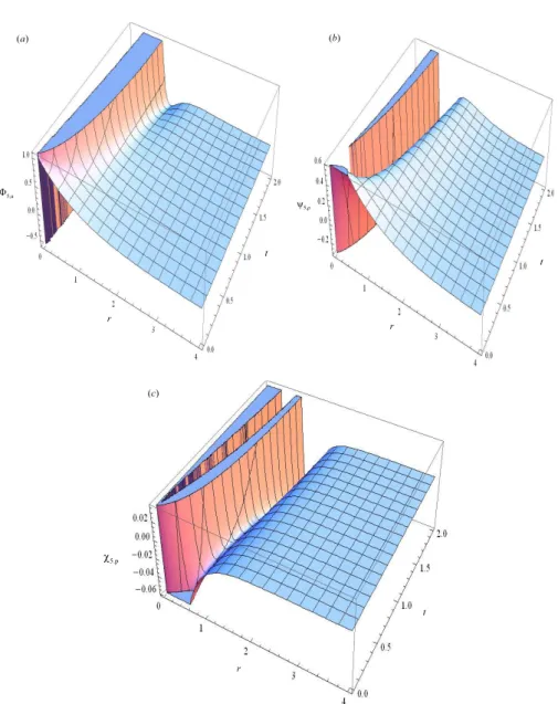
The distribution of flow variables in the flow-field is calculated by the Eqs. (22)– (24) for γ = 1.4 and ν = 1,2,3 for planer, cylindrical and spherical symmetry. For each case of symmetry, the five components of the velocity, density and pressure are computed from the recursive Eqs. (31)–(39) and approximate velocity, density and pressure are given in form of tables and figures.
u0 =e−r,
u1 = 0,
u2 = (−2.93333e−3r+e−4r)t2,
u3 = (−6.93332e−4r+ 1.66667e−5r)t3,
u4 ={(−8.14682 + 0.78222r)e−5r+ (2.96111−0.31111r)e−6r}t4,
and so on. Therefore, the velocity u is given by putting the value of u0, u1,
u2, u3, u4· · ·, in to the Eq. (22). For numerical computation we truncate the
series after five term and the approximate velocity Φ5,u is given by
Φ5,u= 4 X
n=0
un=e−r+ 0 + (−2.93333e−3r +e−4r)t2
+(−6.93332e−4r+ 1.66667e−5r)t3+{(−8.14682 + 0.78222r) +(2.96111−0.31111r)e−6r}t4.
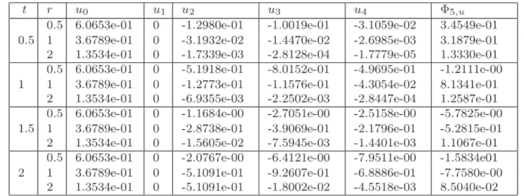
The approximate velocity Φ5,u for ν = 1 is presented in Table 1 and Fig. 1a.
Similarly, for ν = 2 andν = 3 we have computed the five velocity components for different value of r and t and approximate velocity Φ5,u is shown in Tables
4, 7 and Figs. 2a, 3arespectively.
5.2. The density components for planer symmetry ν= 1 are calculated as follows
ρ0 =e−r,
ρ1 = 2e−2rt,
ρ2 = 2e−3rt2,
ρ3 = (3.95555e−4r+ 1.66666e−5r)t3,
ρ4 = (−15.88887e−5r + 8.00000e−6r)t4,
and so on. Therefore, the density distributionρin the flow-field is given by the Eq. (23). The approximate density Ψ5,ρ after truncation up to five term of Eq.
(23) is given by
Ψ5,ρ = 4 X
n=0
ρn=e−r+ 2e−2rt+ 2e−3rt2+ (3.95555e−4r
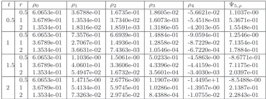
This approximate density Ψ5,ρ for ν = 1 is presented in Table 2 and Fig. 1b.
Similarly, we have computed the approximate density Ψ5,ρ forν = 2 andν = 3
and given into Tables 5, 8 and Figs. 2band 3b respectively for different values of r and t.
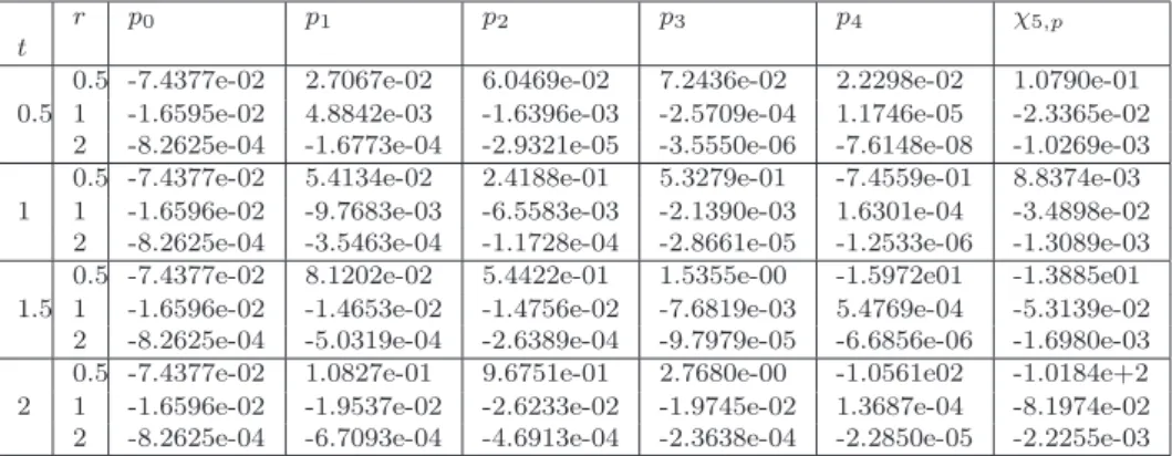
5.3. The pressure components for planer symmetryν = 1 are computed as follows
p0 =−e−3r/3,
p1 = (−1.46667e−4r)t,
p2 = (−3.96000e−5r)t2,
p3 ={(−8.44801 +.52147r)e−6r+ (1.22227r)e−7r}t3,
p4 ={(−1.97074 + 0.96474r)e−7r−(4.86444 + 0.37333r)e−8r}t4,
and so on. So, the pressure distribution p in the flow-field is obtained by Eq. (24). The approximate pressure χ5,p after truncation up to five term of the
decomposition series (24) is
χ5,p= 4 X
n=0
pn= (−0.3333e−3r) + (−1.4667e−4r)t+ (−3.9600e−5r)t2
+{(−8.4480 +.5215r)e−6r+ (1.2223r)e−7r}t3
+{(−1.9707 + 0.9647)e−7r−(4.8644 + 0.3733r)e−8r}t4.
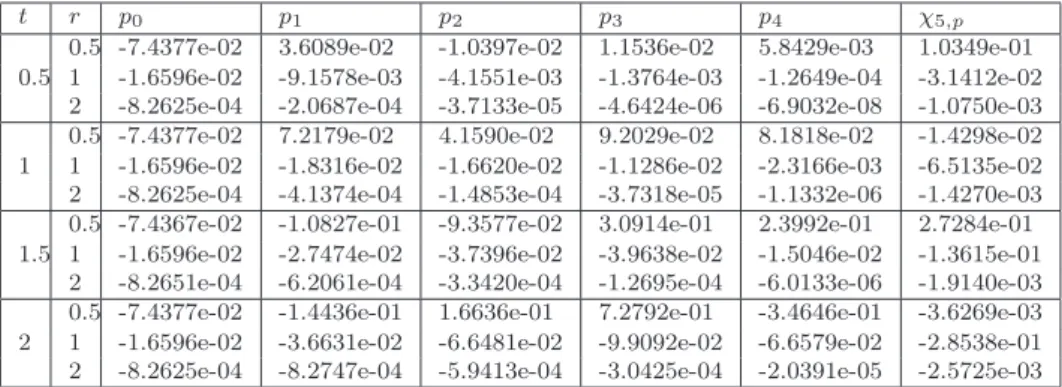
The numerical value of approximate pressure χ5,p for ν = 1 is given in Table
3 and plotted in Fig. 1c. Similarly, the approximate pressure χ5,p for ν = 2
and ν = 3 is given in Tables 6, 9 and Figs. 2c and 3c respectively for different values ofr andt.
t r u0 u1 u2 u3 u4 Φ5,u
0.5 6.0653e-01 0 -1.2980e-01 -1.0019e-01 -3.1059e-02 3.4549e-01 0.5 1 3.6789e-01 0 -3.1932e-02 -1.4470e-02 -2.6985e-03 3.1879e-01 2 1.3534e-01 0 -1.7339e-03 -2.8128e-04 -1.7779e-05 1.3330e-01 0.5 6.0653e-01 0 -5.1918e-01 -8.0152e-01 -4.9695e-01 -1.2111e-00 1 1 3.6789e-01 0 -1.2773e-01 -1.1576e-01 -4.3054e-02 8.1341e-01
2 1.3534e-01 0 -6.9355e-03 -2.2502e-03 -2.8447e-04 1.2587e-01 0.5 6.0653e-01 0 -1.1684e-00 -2.7051e-00 -2.5158e-00 -5.7825e-00 1.5 1 3.6789e-01 0 -2.8738e-01 -3.9069e-01 -2.1796e-01 -5.2815e-01 2 1.3534e-01 0 -1.5605e-02 -7.5945e-03 -1.4401e-03 1.1067e-01 0.5 6.0653e-01 0 -2.0767e-00 -6.4121e-00 -7.9511e-00 -1.5834e01 2 1 3.6789e-01 0 -5.1091e-01 -9.2607e-01 -6.8886e-01 -7.7580e-00
2 1.3534e-01 0 -5.1091e-01 -1.8002e-02 -4.5518e-03 8.5040e-02
Table 1: Variation of the velocity components and approximate velocity Φ5,u
t r ρ0 ρ1 ρ2 ρ3 ρ4 Ψ5,ρ
0.5 6.0653e-01 3.6788e-01 1.6735e-01 1.8605e-02 -5.6621e-02 1.1037e-00 0.5 1 3.6789e-01 1.3534e-01 3.7340e-02 1.6073e-03 -5.4518e-03 5.3671e-01 2 1.3534e-01 1.8316e-02 1.8591e-03 1.3186e-05 -4.2013e-05 1.5548e-01 0.5 6.0653e-01 7.3576e-01 6.6939e-01 1.4884e-01 -9.0594e-01 1.2546e-00 1 1 3.6789e-01 2.7067e-01 1.4936e-01 1.2858e-02 -8.7229e-02 7.1354e-01 2 1.3534e-01 3.6631e-02 7.4363e-03 1.0546e-04 -6.7220e-04 1.7884e-01 0.5 6.0653e-01 1.1036e-00 1.5061e-00 5.0233e-01 -4.5863e-00 -8.6771e-01 1.5 1 3.6789e-01 4.0601e-01 3.3606e-01 4.3396e-02 -4.4159e-01 7.1175e-01
2 1.3534e-01 5.4947e-02 1.6732e-02 3.5601e-04 -3.4030e-03 2.0397e-01 0.5 6.0653e-01 1.4715e-00 2.6776e-00 1.1907e-00 -1.4495e+1 -8.5488e-00 2 1 3.6789e-01 5.4134e-01 5.9745e-01 1.0286e-01 -1.3957e-00 2.1387e-01
2 1.3534e-01 7.3263e-02 2.9745e-02 8.4388e-04 -1.0755e-02 2.2843e-01
Table 2: Variation of the density components and approximate density Ψ5,ρ
with different value of r and tfor planer symmetry ν= 1 and γ = 1.4.
t r p0 p1 p2 p3 p4 χ5,p
0.5 -7.4377e-02 -9.9246e-02 -8.1264e-02 -5.1288e-02 -8.5912e-03 -3.1477e-01 0.5 1 -1.6596e-02 -1.3432e-02 -6.6706e-03 -2.4763e-03 -1.6715e-04 -3.9341e-02 2 -8.2625e-04 -2.4601e-04 -4.4946e-05 -5.7242e-06 -4.1609e-08 -1.1230e-03 0.5 -7.4377e-02 -1.9849e-01 -3.2506e-01 -4.1030e-01 -1.3746e-01 -1.1457e-01 1 1 -1.6596e-02 -2.6863e-02 -2.6682e-02 -1.9810e-02 -2.6744e-03 -9.2625e-02 2 -8.2625e-04 -4.9201e-04 -1.7978e-04 -4.5794e-05 -6.6574e-07 -1.5445e-03 0.5 -7.4377e-02 -2.9774e-01 -7.3136e-01 -1.3848e-00 -6.9589e-01 -3.1842e-00 1.5 1 -1.6596e-02 -4.0294e-02 -6.0035e-02 -6.6859e-02 -1.3539e-02 -1.9732e-01 2 -8.2625e-04 -7.3802e-04 -4.0451e-04 -1.5455e-04 -3.3703e-06 -2.1267e-03 0.5 -7.4377e-02 -3.9698e-01 -1.3002e-00 -3.2824e-00 -2.1993e-00 -7.2533e-00 2 1 -1.6596e-02 -5.3726e-02 -1.0673e-01 -1.5848e-01 -4.2791e-02 -3.7832e-01 2 -8.2625e-04 -9.8402e-04 -7.1914e-04 -3.6635e-04 -1.0652e-05 -2.9064e-03
Table 3: Variation of the pressure components and approximate pressureχ5,p
with different value of r and tfor planer symmetry ν= 1 and γ = 1.4.
Tables 1–3 show that contribution of higher order components in the veloc-ity, density and pressure is comparatively small for all the time t and r ≥1. The common ratioλi=xi+1/xi<1, fori= 0,1,2,3 andx =u,ρ,p; therefore,
the series solution may converge by Adomian decomposition method for planer symmetry. Table 1 and Fig. 1a show that for planer symmetry, the velocity decreases with position for all the timet and r >0.5 and increases steeply for
r < 0.5 for all the time t > 0.5. This show that there exist a discontinuity surface or shock wave in the velocity distribution with respect to position. For the planar symmetry, Table 2 and Fig. 1bshow that the density decreases with position for all timetexcept for 0< r <1. For 0< r <1 andt >1, there exist a discontinuity, i.e. shock wave in distribution of density. Table 3 and Fig. 1c
5,u
Φ ψ5,ρ
5,p
χ
Time t ( )a
( )b
r r
t t
r
t
( )c
t r u0 u1 u2 u3 u4 Φ5,u
0.5 6.0653e-01 0 -7.4377e-03 5.6166e-02 1.2359e-01 7.7885e-01 0.5 1 3.6788e-01 0 -1.9700e-02 -9.1615e-03 -2.6825e-03 3.3634e-01 2 1.3534e-01 0 -1.4295e-03 -2.4791e-04 -2.3911e-05 1.3363e-02 0.5 6.0653e-01 0 -2.9751e-02 4.4933e-01 1.9847e-00 3.0108e-00 1 1 3.6789e-01 0 -7.8799e-02 -7.3288e-02 -4.3809e-02 1.7198e-01 2 1.3534e-01 0 -5.7181e-03 -1.9833e-03 -3.8342e-04 1.2725e-01 0.5 6.0653e-01 0 -6.6939e-02 1.5165e-00 1.0110e01 1.2166e01 1.5 1 3.6789e-01 0 -1.7730e-01 -2.4735e-01 -2.2927e-01 -2.8604e-01
2 1.3534e-01 0 -1.2866e-02 -6.6935e-03 -1.9483e-03 1.1383e-01 0.5 6.0653e-01 0 -1.1900e-01 3.5946e-00 3.2226e01 3.6308e01 2 1 3.6789e-01 0 -3.1520e-01 -5.8631e-01 -7.5776e-01 -1.2914e-00
2 1.3534e-01 0 -2.2872e-02 -1.5866e-02 -6.1893e-03 9.0408e-02
Table 4: Variation of the velocity components and approximate velocity Φ5,u
with different values ofr and tfor cylindrical symmetry ν= 2 and γ = 1.4.
t
r ρ0 ρ1 ρ2 ρ3 ρ4 Ψ5,ρ
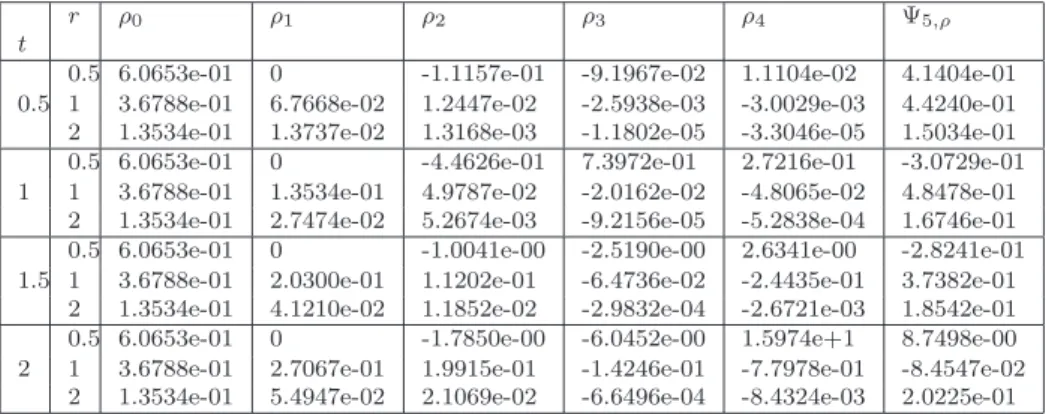
0.5 6.0653e-01 0 -1.1157e-01 -9.1967e-02 1.1104e-02 4.1404e-01 0.5 1 3.6788e-01 6.7668e-02 1.2447e-02 -2.5938e-03 -3.0029e-03 4.4240e-01 2 1.3534e-01 1.3737e-02 1.3168e-03 -1.1802e-05 -3.3046e-05 1.5034e-01 0.5 6.0653e-01 0 -4.4626e-01 7.3972e-01 2.7216e-01 -3.0729e-01 1 1 3.6788e-01 1.3534e-01 4.9787e-02 -2.0162e-02 -4.8065e-02 4.8478e-01
2 1.3534e-01 2.7474e-02 5.2674e-03 -9.2156e-05 -5.2838e-04 1.6746e-01 0.5 6.0653e-01 0 -1.0041e-00 -2.5190e-00 2.6341e-00 -2.8241e-01 1.5 1 3.6788e-01 2.0300e-01 1.1202e-01 -6.4736e-02 -2.4435e-01 3.7382e-01
2 1.3534e-01 4.1210e-02 1.1852e-02 -2.9832e-04 -2.6721e-03 1.8542e-01 0.5 6.0653e-01 0 -1.7850e-00 -6.0452e-00 1.5974e+1 8.7498e-00 2 1 3.6788e-01 2.7067e-01 1.9915e-01 -1.4246e-01 -7.7978e-01 -8.4547e-02
2 1.3534e-01 5.4947e-02 2.1069e-02 -6.6496e-04 -8.4324e-03 2.0225e-01
Table 5: Variation of the density components and approximate density Ψ5,ρ
t r p0 p1 p2 p3 p4 χ5,p
0.5 -7.4377e-02 3.6089e-02 -1.0397e-02 1.1536e-02 5.8429e-03 1.0349e-01 0.5 1 -1.6596e-02 -9.1578e-03 -4.1551e-03 -1.3764e-03 -1.2649e-04 -3.1412e-02
2 -8.2625e-04 -2.0687e-04 -3.7133e-05 -4.6424e-06 -6.9032e-08 -1.0750e-03 0.5 -7.4377e-02 7.2179e-02 4.1590e-02 9.2029e-02 8.1818e-02 -1.4298e-02 1 1 -1.6596e-02 -1.8316e-02 -1.6620e-02 -1.1286e-02 -2.3166e-03 -6.5135e-02 2 -8.2625e-04 -4.1374e-04 -1.4853e-04 -3.7318e-05 -1.1332e-06 -1.4270e-03 0.5 -7.4367e-02 -1.0827e-01 -9.3577e-02 3.0914e-01 2.3992e-01 2.7284e-01 1.5 1 -1.6596e-02 -2.7474e-02 -3.7396e-02 -3.9638e-02 -1.5046e-02 -1.3615e-01
2 -8.2651e-04 -6.2061e-04 -3.3420e-04 -1.2695e-04 -6.0133e-06 -1.9140e-03 0.5 -7.4377e-02 -1.4436e-01 1.6636e-01 7.2792e-01 -3.4646e-01 -3.6269e-03 2 1 -1.6596e-02 -3.6631e-02 -6.6481e-02 -9.9092e-02 -6.6579e-02 -2.8538e-01 2 -8.2625e-04 -8.2747e-04 -5.9413e-04 -3.0425e-04 -2.0391e-05 -2.5725e-03
Table 6: Variation of the pressure components and approximate pressureχ5,p
in flow-field with different values of r and t for cylindrical symmetryν = 2 and γ = 1.4.
For the cylindrical symmetry, Tables 4–6 show that the contribution of higher order components in series solution for velocity, density and pressure distribution are relatively small for all the time tand r≥1. Therefore we can conclude that ratio test for convergence of series will be satisfied and solution of system of gas dynamics equations exist in form of series. The approximate velocity in cylindrical symmetry decrease for allrandt≤1 but fort≥1, it first decreases steeply and then increases with r. Tables 5–6 and Figs. 2b–2c show that there exist multiple discontinuity in distributions of density and pressure for cylindrical symmetry and their position can be identified.
t r u0 u1 u2 u3 u4 Φ5,u
0.5 6.0653e-01 0 1.1492e-01 2.9372e-01 4.8312e-01 1.4983e-00 0.5 1 3.6788e-01 0 -7.4681e-03 -1.8172e-03 7.5676e-04 3.5935e-01 2 1.3534e-01 0 -1.1252e-03 -2.0685e-04 -2.4869e-05 1.3398e-01 0.5 6.0653e-01 0 4.5968e-01 2.3498e-00 7.2158e-00 1.06318e01 1 1 3.6788e-01 0 -2.9872e-02 -1.4538e-02 1.2029e-02 3.3550e-01 2 1.3534e-01 0 -4.5006e-03 -1.6548e-03 -3.9893e-04 1.2878e-01 0.5 6.0653e-01 0 1.0343e-00 7.9305e-00 3.2192e01 4.1763e02 1.5 1 3.6788e-01 0 -6.7213e-02 -4.9065e-02 6.0224e-02 3.1183e-01
2 1.3534e-01 0 -1.0126e-02 -5.5850e-03 -2.0283e-03 1.1760e-01 0.5 6.0653e-01 0 1.8387e-00 1.8798e01 8.2546e01 1.0379e02 2 1 3.6788e-01 0 -1.1949e-01 -1.1630e-01 1.8737e-01 3.1946e-01
2 1.3534e-01 0 -1.8002e-02 -1.3239e-02 -6.4487e-03 9.7646e-02
Table 7: Variation of the velocity components and approximate velocity Φ5,u
in flow-field with different values of r and tfor spherical symmetryν = 3 and
( )a
( )b
( )c
r r
r t
t
t
t
5,u
Φ
5,ρ
ψ
5,p
χ
5,u
Φ
5,ρ
ψ
r
r
t t
( )a ( )b
r
t
5.p
χ
( )c
t
r ρ0 ρ1 ρ2 ρ3 ρ4 Ψ5,ρ
0.5 6.5603e-01 -3.6788e-01 -3.9048e-01 -1.8426e-01 6.3597e-02 -2.7249e-01 0.5 1 3.6788e-01 0 -1.2447e-02 -6.8625e-03 -1.3355e-03 3.4724e-01
2 1.3534e-01 9.1534e-03 7.7461e-04 -3.6891e-05 -2.5382e-05 1.4521e-01 0.5 6.0653e-01 -7.3576e-01 -1.5619e-00 -1.0436e-00 3.1547e-00 4.2028 e-01 1 1 3.6788e-01 0 -4.9787e-02 -5.5346e-02 -2.1813e-02 2.4093e-01
2 1.3534e-01 1.8316e-02 3.0984e-03 -2.9303e-04 -4.0587e-05 1.5605e-01 0.5 6.0653e-01 -1.1036e-00 -3.5143e-00 -1.0979e-00 2.8962e01 2.3853e01 1.5 1 3.6788e-01 0 -1.1202e-01 -1.8930e-01 -1.1529e-01 -4.8734e-02
2 1.3534e-01 2.7474e-02 6.9715e-03 -9.7722e-04 -2.0530e-03 1.6675e-01 0.5 6.0653e-01 -1.4715e-00 -6.2476e-00 5.4390e-00 4.8551e+1 4.6878e01 2 1 3.6788e-01 0 -1.9915e-01 -4.5704e-01 -3.9109e-01 -6.7941e-01
2 1.3534e-01 3.6631e-02 1.2394e-02 -2.2773e-03 -6.4823e-03 1.7560e-01
Table 8: Variation of the density components and approximate density Ψ5,ρ
in flow-field with different values of tand r for spherical symmetryν = 3 and
γ = 1.4.
t
r p0 p1 p2 p3 p4 χ5,p
0.5 -7.4377e-02 2.7067e-02 6.0469e-02 7.2436e-02 2.2298e-02 1.0790e-01 0.5 1 -1.6595e-02 4.8842e-03 -1.6396e-03 -2.5709e-04 1.1746e-05 -2.3365e-02
2 -8.2625e-04 -1.6773e-04 -2.9321e-05 -3.5550e-06 -7.6148e-08 -1.0269e-03 0.5 -7.4377e-02 5.4134e-02 2.4188e-01 5.3279e-01 -7.4559e-01 8.8374e-03 1 1 -1.6596e-02 -9.7683e-03 -6.5583e-03 -2.1390e-03 1.6301e-04 -3.4898e-02
2 -8.2625e-04 -3.5463e-04 -1.1728e-04 -2.8661e-05 -1.2533e-06 -1.3089e-03 0.5 -7.4377e-02 8.1202e-02 5.4422e-01 1.5355e-00 -1.5972e01 -1.3885e01 1.5 1 -1.6596e-02 -1.4653e-02 -1.4756e-02 -7.6819e-03 5.4769e-04 -5.3139e-02
2 -8.2625e-04 -5.0319e-04 -2.6389e-04 -9.7979e-05 -6.6856e-06 -1.6980e-03 0.5 -7.4377e-02 1.0827e-01 9.6751e-01 2.7680e-00 -1.0561e02 -1.0184e+2 2 1 -1.6596e-02 -1.9537e-02 -2.6233e-02 -1.9745e-02 1.3687e-04 -8.1974e-02 2 -8.2625e-04 -6.7093e-04 -4.6913e-04 -2.3638e-04 -2.2850e-05 -2.2255e-03
Table 9: Variation of the pressure components and approximate pressureχ5,p
in flow-field with different values of r and tfor spherical symmetryν = 3 and
γ = 1.4.
is shown in Tables 7–9 and Figures 3a–3c. It is seen that there exist multiple discontinuity (shock wave) in the variation of density and pressure with respect to position.
6. Conclusion
In this paper, Adomian decomposition method is successfully applied for the solution of the system of gas dynamic equations governing the motion of one-dimensional unsteady adiabatic flow of the perfect gas under the variable initial condition for all the three type of symmetry. We have obtained the distribution of approximate velocity, density and pressure directly as function of position and time which was not possible in similarity method. This paper also show the existence of multiple discontinuity or shock wave in the distribution of flow variables and identification of their positions. It is found that the solution of the system of gas dynamic equations by the Adomian decomposition method in form of the series is convergent for a domain of interest. This work show that the Adomian decomposition method can be used in study of one dimensional gas dynamic problem in all the three symmetry with more advanced and realistic gas dynamics problems.
Acknowledgment
The research of the author (Manoj Singh) is supported by UGC, New Delhi, India vide letter no. Sch. No./JRF/AA/139/F-297/2012-13 dated January 22, 2013. The author (Arvind Patel) thanks to the University of Delhi, Delhi India for the R&D grant vide letter no. RC/2015/9677 dated Oct. 25, 2015. The research of third author (Ruchi Bajargaan) is supported by CSIR, New Delhi, India vide letter no. 09/045(1264)/2012-EMR-I.
References
[1] L.I. Sedov,Similarity and Dimensional Methods in Mechanics, Transl. by Morris Friedman (transl. edited by Maurice Holt), Academic Press, New York (1959).
[3] G. Adomian, The diffusion-Brusselator equation,Comput. Math. Appl.,29 (1995), 1-3.
[4] A.-M. Wazwaz, A reliable modification of Adomian decomposition method,
Appl. Math. Comput.,102 (1999), 77-86.
[5] H. Bulut, M. Ergut, V. Asil, and R.H. Bokor, Numerical solution of a viscous incompressible flow problem through an orifice by Adomian de-composition method,Appl. Math. Comput.,153 (2004), 733-741.
[6] H. Li, B. Cheng, and W. Kang, Application of Adomian decomposition method in laminar boundary layer problems of a kind,International Conf. on Control, Automation and Systems Engineering (CASE), July (2011), 30-31, IEEE, doi: 10.1109/ICCASE.5997687.
[7] A.-M. Wazwaz, The modified decomposition method and Pade’ approxi-mants for solving the Thomas-Fermi equation,Appl. Math. Comput.,105 (1999), 11-19.
[8] M. Kumar, and N. Singh, Modified Adomian decomposition method and computer implementation for solving singular boundary value problems arising in various physical problems, Comput. Chem. Eng., 34 (2010), 1750-1760.
[9] F. Chen, and Q. Liu, Modified asymptotic Adomian decomposition method for solving Boussinesq equation of groundwater flow, Appl. Math. Mech., 35(2014), 481-488.
[10] F. Shakeri Aski, S. Nasirkhani, E. Mohammadian, and A. Asgari, Appli-cation of Adomian decomposition method for micropolar flow in a porous channel,Appl. Math. Mech.,3(2014), 15-21.
[11] G. Adomian, Nonlinear Stochastic Operator Equations, Academic Press, Orlando, FL (1986).
[12] G. Adomian, Solving Frontier Problems of Physics: The Decomposition Method, Kluwer, Boston (1994).
[14] S. Nourazar, M. Ramezanpour, and A. Doosthoseini, A new algorithm to solve the gas dynamics equation: an application of the Fourier transform Adomian decomposition method,Appl. Math. Sci. (Ruse),7(2013), 4281-4286.
[15] M.A. Mohamed, Adomain decomposition method for solving the equation governing the unsteady flow of polytropic gas, Application and Applied Mathematics,4 (2009), 52-61.
[16] G. Adomian, A review of the decomposition method in applied mathemat-ics,J. Math. Anal. Appl.,135(1988), 501-544.
[17] A.-M. Wazwaz, The decomposition method for approximate solution of the Goursat problem.Appl. Math. Comput., 69(1995), 299-311.
[18] V. Seng, K. Abbaoui, and Y. Cherruault, Adomian’s polynomials for non-linear operators,Math. Comput. Modelling,24(1996), 59-65.
[19] A.-M. Wazwaz, A new algorithm for calculating Adomian polynomials for nonlinear operators, Appl. Math. Comput.,111 (2000), 53-69.