Many-Core Approaches to Combinatorial Problems: case of the Langford Problem

Many-Core Approaches to Combinatorial Problems: case of the

Langford problem

M. Krajecki1_{, J. Loiseau}1_{, F. Alin}1_{, C. Jaillet}1

c

The Author 2017. This paper is published with open access at SuperFri.org

As observed from the last TOP5002 list - November 2015 -, GPUs-accelerated clusters emerge as clear evidence. But exploiting such architectures for combinatorial problem resolution remains a challenge.

In this context, this paper focuses on the resolution of an academic combinatorial problem, known as the Langford pairing problem, which can be solved using several approaches. We first focus on a general solving scheme based on CSP (Constraint Satisfaction Problem) formalism and backtrack called the Miller algorithm. This method enables us to compute instances up toL(2,21) using both CPU and GPU computational power with load balancing.

As dedicated algorithms may still have better computation efficiency we took advantage of Godfrey’s algebraic method to solve the Langford problem and implemented it using our multiGPU approach. This allowed us to recompute the last open instances,L(2,27) andL(2,28), respectively in less than 2 days and 23 days using best-effort computation on the ROMEO3 _{supercomputer} with up to 500,000 GPU cores.

Keywords: Combinatorial problems, parallel algorithm, GPU accelerators, CUDA, Langford problem.

Introduction

For many years now, GPUs usage has increased in the field of High Performance Computing. The TOP500 list of the world’s most powerful supercomputers contains more than 52 systems powered by NVIDIA Kepler GPUs. In the latest list a number of hybrid machines increased compared fourfold with the previous list.

Since 2007, NVIDIA has offered a general GPUs programming interface: Compute Unified

De-vice Architecture (CUDA). This study is based on this physical and logical architecture which

requires massively parallel programming and a new vision for the implementation of resolution algorithms.

The Langford pairing problem is a very irregular combinatorial problem and thus is a bad candidate for GPU computation which requires vectorized and regularized tasks. Hopefully there are many ways to regularize the computation in order to take advantage of the multiGPU cluster architectures.

This paper is structured as follows: we first present the background with the Langford problem and multiGPU cluster. The next section describes our method concerning the Miller algorithm on such architectures. Then we expose our multiGPU solution to solve the Langford problem based on the Godfrey algorithm. Finally, we present some concluding remarks and perspectives.

1_{University of Reims Champagne-Ardenne, Reims, France} 2_{http://www.top500.org}

3_{https://romeo.univ-reims.fr/pages/aboutUs}

Table 1.Solutions and time with differents methods

Instance Solutions Method Computation time

L(2,3) 1 Miller algorithm

-L(2,4) 1

-... ... ...

L(2,16) 326,721,800 120 hours

L(2,19) 256,814,891,280 2.5 years (1999) DEC Alpha L(2,20) 2,636,337,861,200 Godfrey algorithm 1 week L(2,23) 3,799,455,942,515,488 4 days with CONFIIT L(2,24) 46,845,158,056,515,936 3 months with CONFIIT

L(2,27) 111,683,611,098,764,903,232

-L(2,28) 1,607,383,260,609,382,393,152

-1. Background

1.1. Langford problem

C. Dudley Langford gave his name to a classic permutation problem [1, 2]. While observing his son manipulating blocks of different colors, he noticed that it was possible to arrange three pairs of different colored blocks (yellow, red, blue) in such a way that only one block separates the red pair - noted as pair 1 - , two blocks separate the blue pair - noted as pair 2 - and finally three blocks separate the yellow one - noted as pair 3 - , see Fig. 1.

Yellow

(3) Red(1) Blue(2) Red(1) Yellow(3) Blue(2)

Figure 1. L(2,3) arrangement

This problem has been generalized to any number n of colors and any number sof blocks having the same color. L(s, n) consists in searching for the number of solutions to the Langford problem, up to a symmetry. In November 1967, Martin Gardner presented L(2,4) (two cubes and four colors) as being part of a collection of small mathematical games and he stated that

L(2, n) has solutions for all n such that n = 4k or n = 4k₋1 (k _∈ N_{\ {}0_}). The central resolution method consists in placing the pairs of cubes, one after the other, on free places and backtracking if no place is available (see Fig. 3 for a detailed algorithm).

The Langford problem has been approached in different ways: discrete mathematics re-sults, specific algorithms, specific encoding, constraint satisfaction problem (CSP), inclusion-exclusion . . . [3–6]. In 2004, the last solved instance,L(2,24), was computed by our team using a specific algorithm. (see Table 1); L(2,27) andL(2,28) have just been computed but no details were given.

Then, we use the Godfrey method to achieveL(2,24) more quickly and then recomputeL(2,27) and L(2,28), presently known as the last instances. The Larsen method is based on inclusion-exclusion [6]; although this method is effective, practically the Godfrey technique is better. The lastest known work on the Langford Problem is a GPU implementation proposed in [7] in 2015. Unfortunately this study does not provide any performance considerations but just gives the number of solutions of L(2,27) andL(2,28).

1.2. MultiGPU clusters and the ROMEO supercomputer

GPUs always come with CPUs which delegate them part of their computation. Let us consider a cluster as a set of one CPU and one or more GPU(s), which we call machines. We see these clusters as 3-level parallelism structures (as described in 2.1.4), with communications between nodes and/or machines, CPUs that prepare computation and finally delegate part of it to the GPUs. When the problem can be split into a finite number of independent tasks, it is possible to distribute them over the machines. That permits to make an efficient use of the cluster hardware. Depending on the way of computation submission we can use either a static multinode reservation with one job including MPI client-server tasks dis-tribution, or a best-effort dynamic reservation using several one-node jobs for independent tasks.

As the execution model of GPUs is based on SIMT (Single Instruction Multiple Threads), the same instruction flow is shared by all the threads that execute synchronously by warp

teams [8, 9]. The divergences in this flow are handled by the NVIDIA GPUs scheduler, but lead to synchronization between threads and an efficiency loss. This is the reason why we intend to provide regular resolution algorithms for an efficient use of the GPU capabilities and, moreover, with multiGPU clusters.

ROMEO supercomputer - All the tests below were led on the ROMEO cluster available at

the University of Reims Champagne-Ardenne (France). It provides 130 nodes, each composed of 2 Ivy Bridge CPUs (8 cores), 2.6GHz and 2 Tesla K20Xm GPUs.

We use the nodes as two independent machines with one eight core CPU and one GPU attached, linked by PCIe-v3. This allows having 260 machines for computation, each containing 32GB RAM memory. A K20Xm GPU has 6GB memory, 250GB/s of bandwidth, 2688 CUDA cores including 896 double precision cores.

2. Miller algorithm

In this part we present our multiGPU cluster implementation of the Miller’s algorithm. First, we introduce the backtrack method. Then we present our implementation in order to fit the GPUs architecture. The last section presents our results.

2.1. Backtrack resolution

2.1.1. Langford’s problem tree representation

In [10], we propose to formalize the Langford problem as a CSP (Constraint Satisfaction

Problem), first introduced by Montanari in [11], and show that an efficient parallel resolution is

possible. CSP formalized problems can be transformed into tree evaluations. In order to solve

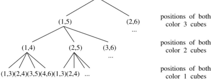
L(2, n), we consider the following tree of height n: see example ofL(2,3) in Fig. 2.

color 1 cubes positions of both positions of both

color 3 cubes

color 2 cubes positions of both

(1,3)(2,4)(3,5)(4,6)(1,3)(2,4) ... ...

(1,5) (2,6)

...

(1,4) (2,5) (3,6)

Figure 2. Search tree forL(2,3)

• Every level of the tree corresponds to a color.

• Each node of the tree corresponds to the placement of a pair of cubes without worrying about the other colors. Color p is represented at depth n₋p+ 1, where the first node corresponds to the first possible placement (positions 1 andp+2) andith_{node corresponds}

to the placement of the first cube of color p in positioni, i_∈[1, 2n₋1₋p].

• Solutions are leaves generated without any placement conflict.

There are many ways to browse the tree and find the solutions: backtracking,

forward-checking,backjumping, etc [12]. We limit our study to the naivebacktrack resolution and choose

to evaluate the variables and their values in a static order; in a depth-first manner, the solutions are built incrementally and if a partial assignment can be aborted, the branch is cut. A solution is found each time a leaf is reached.

The recommendation for performance on GPU accelerators is to use non test-based pro-grams. Due to its irregularity, the basic backtracking algorithm, presented on Fig. 3, is not supposed to suit the GPU architecture. Thus a vectorized version is given when evaluating the assignments at the leaves’ level, with one of the two following ways: assignments can be pre-pared on each tree node or totally set on final leaves before testing the satisfiability of the built solution (Fig. 4).

while not done do

test pair <- test

if successful then if max depth then

count solution higher pair else

lower pair <- remove else

higher pair <- add

Figure 3.Backtrack algorithm

for pair 1 positions

assignment <- add

for pair 2 positions

assignment <- add

for ...

for pair n positions

assignment <- add

if final test ok then count solution

2.1.2. Data representation

In order to count every Langford problem solution, we first identify all possible combinations for one color without worrying about the other ones. Each possible combination is coded within an interger, one bit to 1 corresponding to a cube presence, a 0 to its absence. This is what we called a mask. This way Fig. 5 presents the possible combinations to place the one, two and three weight cubes for theL(2,3) Langford instance.

Furthermore, the masks can be used to evaluate the partial placements of a chosen set of colors: all the 1s correspond to occupied positions; the assignment is consistent iff there are as many 1s as the number of cubes set for the assignment.

With the aim to find solutions, we just have to go all over the tree andsum one combination of each of the colors: a solution is foundiff all the bits of the sum are set to 1.

Each route on the tree can be evaluated individually and independently; then it can be evaluated as a thread on the GPU. This way the problem is massively parallel and can be, indeed, computed on GPU. Fig. 6 represents the tree masks’ representation.

0 0 0 1 0 1

0 0 1 0 1 0 0 1 0 1 0 0

1 0 1 0 0 0

0 0 1 0 0 1

0 1 0 0 1 0

1 0 0 1 0 0

0 1 0 0 0 1 1 0 0 0 1 0

pair 1 pair 2 pair 3

1 2 3 4

Figure 5. Bitwise representation of pairs positions inL(2,3)

... ...

0 0 0 0 ]

...

0 0 00 0 0

0

0 0

0 1 1 1

1

0

1 1 1 1 1 01 1

0 0 0 0 [1 1

1 1 1 1 1 1 1 1 1 1

1 1 1 1 1

Figure 6. Bitwise representation of the Langford

L(2,3) placement tree

2.1.3. Specific operations and algorithms

Three main operations are required in order to perform the tree search. The first one, used for both backtrack and regularized methods, aims to add a pair to a given assignment. The second one, allowing to check if a pair can be added to a given partial assignment, is only necessary for the original backtrack scheme. The last one is used for testing if a global assignment is an available solution: it is involved in the regularized version of the Miller algorithm.

Add a pair -Top of Fig. 7 presents the way to add a pair to a given assignment. With a

binary or, the new mask contains the combination of the original mask and of the added pair.

This operation can be performed even if the position is not available for the pair (however the resulting mask is inconsistent).

Test a pair position - On the bottom part of the same figure, we test the positioning of

a pair on a given mask. For this, it is necessary to perform a binary and between the mask and the pair.

= 0: success, the pair can be placed here

6

= 0: error, try another position

Final validity test - The last operation is for a posteriori checking. For example the

Using this data representation, we implemented both backtrack and regularized versions of the Miller algorithm, as presented in Fig. 3 and 4.

The next section presents the way we hybridize these two schemes in order to get an efficient parallel implementation of the Miller algorithm.

2.1.4. Hybrid parallel implementation

This part presents our methodology to implement Miller’s method on a multiGPU cluster.

Tasks generation - In order to parallelize the resolution we have to generate tasks.

Con-sidering the tree representation, we construct tasks by fixing the different values of a first set of variables [pairs] up to a given level. Choosing the development level allows to generate as many tasks as necessary. This leads to a Finite number of Irregular and Independent Tasks (FIIT

applications [13]).

Cluster parallelization - The generated tasks are independent and we spread them in

a client-server manner: a server generates them and makes them available for clients. As we consider the cluster as a set of CPU-GPU(s) machines, the clients are these machines. At the machine level, the role of the CPU is, first, to generate work for the GPU(s): it has to generate sub-tasks, by continuing the tree development as if it were a second-level server, and the GPU(s) can be considered as a second-level client(s).

The sub-tasks generation, at the CPU level, can be made in parallel by the CPU cores. Depend-ing on the GPUs number and their computation power the sub-tasks generation rhythm may be adapted to maintain a regular workload both for the CPU cores and GPU threads: some CPU cores, not involved in the sub-tasks generation, could be made available for sub-tasks computing. This leads to the 3-level parallelism scheme presented in Fig. 8, where p, q and r respectively correspond to: (p) the server-level tasks generation depth, (q) the client-level sub-tasks genera-tion one, (r) the remaining depth in the tree evaluation, i.e.the number of remaining variables to be set before reaching the leaves.

Backtrack and regularized methods hybridization - The Backtrack version of the Miller algorithm suits CPU execution and allows to cut branches during the tree evaluation, reducing the search space and limiting the combinatorial explosion effects. A regularized version must be developed, since GPUs execution requires synchronous execution of the threads, with as few branching divergence as possible; however, this method imposes to browse the entire search space and is too time-consuming.

We propose to hybridize two methods in order to take advantage of both of them for the multiGPU parallel execution: for tasks and sub-tasks generated at sever and client levels, the tree development by the CPU cores is made using the backtrack method, cutting branches as soon as possible [and generating only possible tasks]; when computing the sub-tasks generated at client-level, the CPU cores involved in the sub-tasks resolution use the backtrack method and the GPU threads the regularized one.

2.2. Experiments tuning

b) testing a pair mask

pair and

10 10 1 1

0 10 10 0 = 0

and 10 10 1 1 0 0 0 10 1

= 1 a) adding a pair

mask pair or

10 10 1 1

0 10 10 0

1 1 1 1 1 1

or 10 10 1 1 0 0 0 10 1 1 0 1 1 1 1

Figure 7.Testing and adding position

Client Server

GPUs CPUs

masks generated on the server

masks generated by clients

p

q

r

Figure 8.Server client distribution

Figure 9.Time depending on grid and block size on n= 15

2.2.1. Registers, blocks and grid

In order to use all GPUs capabilities, the first way was to fill the blocks and a grid. To maximize occupancy (ratio between active warps and the total number of warps) NVIDIA suggests to use 1024 threads per block to improve GPU performances and proposes a CUDA occupancy calculator4_{. But, confirmed by the Volkov’s results [14], we experimented that better} performances may be obtained using lower occupancy. Indeed, another critical criterion is the inner GPU registers occupation. The optimal number of registers (57 registers) is obtained by setting 9 pairs placed on the client forL(2,15), thus 6 pairs are remaining for GPU computation. In order to tune the blocks and grid sizes, we performed tests on the ROMEO architecture. Fig. 9 represents the time in relation with a number of blocks per grid and a number of threads per block. The most relevant result, observed as a local minimum on the 3D surface, is obtained near 64 or 96 threads per block; for the grid size, the limitation is relative to the GPU global memory size. It can be noted that we do not need shared memory because their are no data exchanges between threads. This allows us to use the total available memory for the L1 cache for each thread.

2.2.2. Streams

A client has to prepare work for GPU. There are four main steps: generate tasks, load them into the device memory, process the task on the GPU and then get results.

CPU-GPU memory transfers cause huge time penalties (about 400 cycles latency for trans-fers between CPU memory and GPU device memory). At first, we had no overlapping between memory transfer and kernel computation because the tasks generation on CPU was too long compared to the kernel computation. To reduce the tasks generation time we used OpenMP in order to use eight available CPU cores. Thus, CPU computation was totally hidden by memory transfers and GPU kernel computation. We tried using up to 7 streams; as shown by Fig. 10, using only two simultaneous streams did not improve efficiency, because the four steps did not overlap completely; the best performances were obtained with three streams; the slow increase in the next values is caused by synchronization overhead and CUDA streams management.

Figure 10. Computing time depending on

streams number

1 2 3 4 5 6 7 8

100 120 140 160 180 200 220 240 260 280 300

Reference: 100% CPU best performance 100% GPU computing, CPU cores only feeding CPU+GPU, CPU core feeding GPU (free core computing)

Number of CPU cores feeding GPU

Ti

m

e

(

s)

Figure 11.CPU cores optimal distribution for GPU feeding

2.2.3. Setting up the server, client and GPU depths

We now have to set the depths of each actor, server (p), client (q) and GPU (r) (see Fig. 8). First we set ther= 5 for large instances because of the GPU limitation in terms of registers by threads, exacerbated by the use of numerous 64bits integers. For r _≥ 6, we get too many registers (64) and for r _≤ 4 the GPU computation is too fast compared to the memory load overhead.

Clients are the buffers between the server and the GPUs: q = n₋p₋r. So we have conducted tests by varying the server depth, p. The best result is obtained for p = 3 and performance decreases quickly for higher values. This can be explained since more levels on the server generates smaller tasks; thus GPU use is not long enough to overlap memory exchanges.

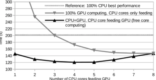
2.2.4. CPU: Feed the GPUs and compute

2.3. Results

2.3.1. Regularized method results

We now can show the results obtained for our massively parallel scheme using the previous optimizations, comparing the computation times of successive instances of the Langford problem. These tests were performed on 20 nodes of the ROMEO supercomputer, hence 40 CPU/GPU machines.

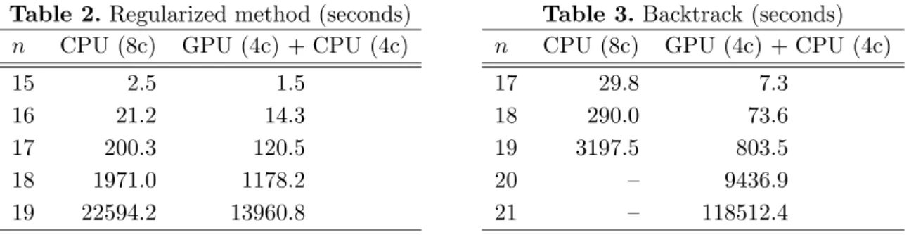
The previous limit with Miller’s algorithm was L(2,19), obtained in 1999 after 2.5 years of sequential effort and at the same time after 2 months with a distributed approach [3]. Our computation scheme allowed us to obtain it in less than 4 hours (Table 2), this being not only due to Moore law progress.

Note that the computation is 1.6 faster with CPU+GPU together than using 8 CPU cores. In addition, the GPUs compute 200000× more nodes of the search tree than the CPUs, with a faster time.

Table 2. Regularized method (seconds)

n CPU (8c) GPU (4c) + CPU (4c)

15 2.5 1.5

16 21.2 14.3

17 200.3 120.5 18 1971.0 1178.2 19 22594.2 13960.8

Table 3.Backtrack (seconds)

n CPU (8c) GPU (4c) + CPU (4c)

17 29.8 7.3

18 290.0 73.6

19 3197.5 803.5

20 – 9436.9

21 – 118512.4

The computation time between two different consecutive instances being multiplied by 10 approximately, this could allow us to obtain L(2,20) in a reasonable time.

2.3.2. Backtracking on GPUs

It appears at first sight that using backtracking on GPUs without any regularization is a bad idea due to threads synchronization issues. But in order to compare CPU and GPU computation power in the same conditions we decide to implement the original backtrack method on GPU (see Fig. 3) with only minor modifications. In these conditions we observe very efficient work of the NVIDIA scheduler, which perfectly handles threads desynchronization. Thus we use the same server-client distribution as in 2.1.4, each client generates masks for both CPU and GPU cores. The workload is then statically distributed on GPU and CPU cores. Executing the backtrack algorithm on a randomly chosen set of sub-problems allowed us to set the GPU/CPU distribution ratio experimentally to 80/20%,

The experiments were performed on 129 nodes of the ROMEO supercomputer, hence 258 CPU/GPU machines and one node for the server. Table 3 shows the results with this config-uration. This method first allowed us to perform the computation of L(2,19) in less than 15 minutes, 15_× faster than with the regularized method; then, we pushed the limitations of the Miller algorithm up toL(2,20) in less than 3 hours and evenL(2,21) in about 33 hours5.

This exhibits the ability of the GPU scheduler to manage highly irregular tasks. It proves that GPUs are adapted even to solve combinatorial problems, which they were not supposed to do.

3. Godfrey’s algebraic method

The previous part presents the Miller algorithm for the Langford problem, this method cannot achieve bigger instances than theL(2,21).

An algebraic representation of the Langford problem has been proposed by M. Godfrey in 2002. In order to break the limitation of L(2,24) we already used this very efficient problem specific method. In this part we describe this algorithm and optimizations, and our implementation on multiGPU clusters.

3.1. Method description

Consider L(2,3) and X = (X1, X2, X3, X4, X5, X6). It proposes to modelize L(2,3) by

F(X,3) = (X1X3+X2X4+X3X5+X4X6)×(X1X4+X2X5+X3X6)×(X1X5+X2X6) In this approach each term represents a position of both cubes of a given color and a solution to the problem corresponds to a term developed as (X1X2X3X4X5X6); thus the number of solutions is equal to the coefficient of this monomial in the development. More generally, the solutions to L(2, n) can be deduced from (X1X2X3X4X5...X2n) terms in the development of

F(X, n).

If G(X, n) =X1...X2nF(X, n) then it has been shown that: P

(x1,...,x2n)∈{−1,1}2n

G(X, n)_(x1,...,x2n) = 22n+1L(2, n)

So P

(x1,...,x2n)∈{−1,1}2n 2n Q i=1

xi n Q i=1

2n−_Pi−1

k=1

xkxk+i+1 = 22n+1L(2, n)

That allows to getL(2, n) from polynomial evaluations. The computational complexity ofL(2, n) is of O(4n _×n2_{) and an efficient big integer arithmetic is necessary. This principle can be} optimized by taking into account the symmetries of the problem and using the Gray code: these optimizations are described below.

3.2. Optimizations

Some works focused on finding optimizations for this arithmetic method [15]. Here we explain the symmetric and computation optimizations used in our algorithm.

3.2.1. Evaluation parity

As [F(−X, n) = F(X, n)], G is not affected by a global sign change. In the same way the global sign does not change if we change the sign of each pair or impair variable.

3.2.2. Symmetry summing

In this problem we have to count each solution up to a symmetry; thus for the first pair of cubes we can stop the computation at half of the available positions considering

S₁0(x) =Pn_k=1−1xkxk+2 instead ofS1(x) =P2k=1n−2xkxk+2. The result is divided by 2.

3.2.3. Sums order

Each evaluation ofSi(x) =P_k2n₌₁−i−1xkxk+i+1, before multiplying might be very important regarding to the computation time for this sum. Changing only one value of xi at a time, we

can recompute the sum using the previous one without global recomputation. Indeed, we order the evaluations of the outer sum using Gray code sequence. Then the computation time is considerably reduced.

Based on all these improvements and optimizations we can use the Godfrey method in order to solve huge instances of the Langford problem. The next section develops the main issues of our multiGPU architecture implementation.

3.3. Implementation details

In this part we present specific adaptations required to implement the Godfrey method on a multiGPU architecture.

3.3.1. Optimized big integer arithmetic

In each step of computation, the value of eachSi can reach 2n−i−1 in absolute value, and

their product can reach (2_(nn₋−_2)!2)!. As we have to sum the Si product on 22n values, in the worst

case we have to store a value up to 22n(2n−2)!

(n−2)!, which corresponds to 1061 forn= 28, with about 200 bits.

So we need few big integer arithmetic functions. After testing existing libraries like GMP for CPU or CUMP for GPU, we have come to the conclusion that they implement a huge number of functionalities and are not really optimized for our specific problem implementation: product of ”small” values and sum of ”huge” values.

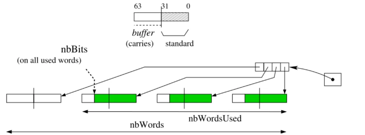
Finally, we developed a light CPU and GPU library adapted to our needs. In the sum for example, as maintaining carries has an important time penalty, we have chosen to delay the spread of carries by using buffers: carries are accumulated and spread only when useful (for example when the buffer is full). Fig. 12 represents this big integer handling.

nbWords 00000 00000 00000 11111 11111 11111

0 31 63

buffer

(carries) standard

nbBits

(on all used words)

nbWordsUsed

3.3.2. Gray sequence in memory

The Gray sequence cannot be stored in an array, because it would be too large (it would contain 22nbyte values). This is the reason why only one part of the Gray code sequence is stored in memory and the missing terms are directly computed from the known ones using arithmetic considerations. The size of the stored part of the Gray code sequence is chosen to be as large as possible to be contained in the processor’s cache memory, the L1 cache for the GPUs threads: so the accesses are fastened and the computation of the Gray code is optimized. For an efficient use of the E5-2650 v2 ROMEO’s CPUs, which disposes of 20 MB of level-3 cache, the CPU Gray code sequence is developed recursively up to depth 25. For the K20Xm ROMEO’s GPUs, which dispose of 8 KB of constant memory, the sequence is developed up to depth 15. The rest of the memory is used for the computation itself.

3.3.3. Tasks generation and computation

In order to perform the computation of the polynomial, two variables can be set among the 2n available. For the tasks generation we choose a number p of variables to generate 2p tasks by developing the evaluation tree to depth p.

The tasks are spread over the cluster, either synchronously or asynchronously.

Synchronous computation -The first experiment was carried out with an MPI

distribu-tion of tasks of the previous model. Each MPI process finds its tasks list based on its processid; then converting each task number into binary gives the task’s initialization. The processes work independently; finally the root process (id = 0) gathers all the computed numbers of solutions and sums them.

Asynchronous computation - In this case the tasks can be computed independently. As

with the synchronous computation, the tasks’ initializations are retrieved from their number. Each machine can get a task, compute it, and then store its result; then when all the tasks have been computed, the partial sums are added together and the total result is provided.

3.4. Experimental settings

This part presents the experimental context and methodology, and the way experiments were carried out. This study has similar goals as for the Miller’s resolution experiments.

3.4.1. Experimental methodology

We present here the way the experimental settings were chosen. Firstly, we define the tasks distribution, secondly, we set the number of threads per GPU block; finally, we set the CPU/GPU distribution.

Tasks distribution depth -This value being set it is important to get a high number of

blocks to maintain sufficient GPU load. Thus, we have to determine the best number of tasks for the distribution. As presented in part 3.3.3, the number p of bits determines 2p _{tasks. On}

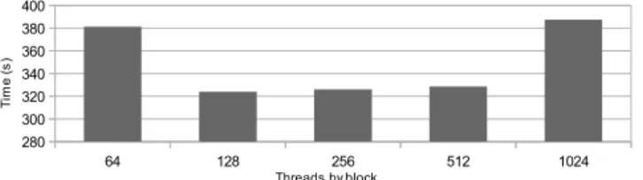
Number of threads per block - In order to take advantage of the GPU computation power, we have to determine the threads/block distribution. Inspired by our experiments with Miller’s algorithm we know that the best value may appear at lower occupancy. We perform tests on a given tasks set varying the threads/block number and grid size associated. Fig. 13 presents the tests performed on then= 20 problem: the best distribution is around 128 threads per block.

64 128 256 512 1024

280 300 320 340 360 380 400

Threads by block

T im e ( s )

Figure 13.L(2,20), number of threads per block

22 23 24 25 26 27 28 29 30 31

15000 15200 15400 15600 15800 16000 16200 16400

server computing depth

L (2 ,2 3 ) co m p u tin g ti m e ( s)

Figure 14.Influence on server generation depth

60 62 64 66 68 70 72

14500 14900 15300 15700 16100 16500

% tasks computed by the GPU

L (2 ,2 3 ) co m p u tin g ti m e ( s)

Figure 15.Influence of tasks repartition

CPU vs GPU distribution - The GPU and CPU computation algorithm will approximately

be the same. In order to take advantage of all the computational power of both components we have to balance tasks between CPU and GPU. We performed tests by changing the CPU/GPU distribution based on simulations on a chosen set of tasks. Fig. 15 shows that the best distribution is obtained when the GPU handles 65% of the tasks. This optimal load repartition directly results from the intrinsics computational power of each component; this repartition should be adapted if using a more powerful GPU like Tesla K40 or K80.

3.4.2. Computing context

As presented in part 1.2, we used the ROMEO supercomputer to perform our tests and computations. On this supercomputer SLURM [16] is used as a reservation and a job queue manager. This software allows two reservation modes: a static one-job limited reservation or an opportunity to dynamically submit several jobs in a Best-Effort manner.

Static distribution -In this case we used the synchronous distribution presented in 3.3.3.

We submited a reservation with the number of MPI processes and the number of cores per process. This method is useful to get the results quickly if we can get at once a large amount of computation resources. It was used to perform the computation of small problems, and even for

L(2,23) andL(2,24).

As an issue, it has to be noted that it is difficult to quickly obtain a very large reservation on such a shared cluster, since many projects are currently running.

Best effort - SLURM allows to submit tasks in the specific Best-Effort queue, which does

reservation is set for a job in the best effort queue for a minimum time reservation. If another user asks for a reservation and requests this node, the best effort job is killed (with, for example, a SIGTERM signal). This method, based on asynchronous computation, enables a maximal use of the computational resources without blocking for a long time the entire cluster.

For L(2,27) and even more for L(2,28) the total time required is too important to use the whole machine off a challenge period, thus we chose to compute in a Best-Effort manner. In order to fit with this submission method we chose a reasonable time-per-task, sufficient to optimize the treatments with low loading overhead, but not too long so that killed tasks are not too penalizing for the global computation time. We empirically chose to run 15-20 minute tasks and thus we consideredp= 15 forn= 27 and p= 17 forn= 28.

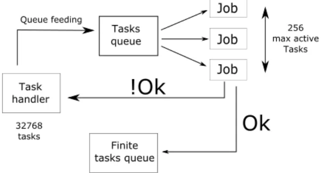
The best effort based algorithm is presented on Fig. 16. The task handler maintains a maximum of 256 tasks in the queue; in addition the entire process is designed to be fault-tolerant since killed tasks have to be launched again. When finished, the tasks generate an ouput containing the number of solutions and computation time, that is stored as a file or database entry. At the end the outputs of the different tasks are merged and the global result can be provided.

Ok

!Ok

Job

256 max active

Tasks

Tasks queue

Task handler

32768 tasks

Finite tasks queue

Queue feeding

Job

Job

Figure 16.Best-effort distribution

3.5. Results

After these optimizations and implementation tuning steps, we conducted tests on the ROMEO supercomputer using best-effort queue to solve L(2,27) and L(2,28). We started the experiment after an update of the supercomputer, that implied a cluster shutdown. Then the machine was restarted and was about 50% idle for the duration of our challenge. The com-putation lasted less than 2 days for L(2,27) and 23 days for L(2,28). The following describes performances considerations.

Computing effort - For L(2,27), the effective computation time of the 32,768 tasks was

about 30 million seconds (345.4 days), and 165,000” elapsed time (1.9 days); the average time of the tasks was 911”, with a standard deviation of 20%. For theL(2,28) 131,072 tasks the total computation time was about 1365 days (117 million seconds), as 23 day elapsed time; the tasks lasted 1321” on average with a 12% standard deviation.

Best-effort overhead -WithL(2,27) we used a specific database to maintain information

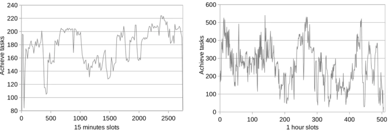
Cluster occupancy -Fig. 17 presents the tasks resolution over the two computation days for L(2,27). The experiment elapse time was 164700” (1.9 days). Compared to the effective computation time, we used an average of 181.2 machines (CPU-GPU couples): this represents 69.7% of the entire cluster.

Fig. 18 presents the tasks resolution flow during the 23 days computation for L(2,28). We used about 99 machines, which represents 38% of 230 available nodes.

0 500 1000 1500 2000 2500 80

100 120 140 160 180 200 220 240

15 minutes slots

A

ch

ie

ve

ta

sk

s

Figure 17.L(2,27) tasks grouped by 15” slots

0 100 200 300 400 500 0

100 200 300 400 500 600

1 hour slots

A

ch

ie

ve

ta

sk

s

Figure 18.L(2,28) tasks grouped by 1 hour slots

For L(2,27), these results confirm that the computation took great advantage of the low occupancy of the cluster during the experiment. This allowed us to obtain a weak best-effort overhead, and an important cluster occupancy. Unfortunately, forL(2,28) on such a long period we got a lower part of the supercomputer dedicated to our computational project. Thus, we are confident in good perspectives for the L(2,31) instance if computed on an even larger cluster or several distributed clusters.

Conclusion

This paper presents two methods to solve the Langford pairing problem on multiGPU clus-ters. In its first part the Miller’s algorithm is presented. Then to break the problem limitations we show optimizations and implementation of Godfrey’s algorithm.

CSP resolution method -As any combinatorial problem can be represented as a CSP, the

Miller algorithm can be seen as a general resolution scheme based on the backtrack tree browsing. A three-level tasks generation allows to fit the multiGPU architecture. MPI or Best-Effort are used to spread tasks over the cluster, OpenMP for the CPU cores distribution and then CUDA to take advantage of the GPU computation power. We were able to compute L(2,20) with this regularized method and to get an even better time with the basic backtrack. This proves the proposed approach and also exhibits that the GPU scheduler is very efficient at managing highly divergent threads.

MultiGPU clusters and best-effort -In addition and with the aim to beat the Langford

Langford problem results - This study enabled us to compute L(2,27) and (L2,28) in respectively less than 2 days and 23 days on the University of Reims ROMEO supercomputer. The total number of solutions is:

L(2,27) = 111,683,611,098,764,903,232 L(2,28) = 1,607,383,260,609,382,393,152

Perspectives -This study shows the benefit of using GPUs as accelerators for combinatorial

problems. In Miller’s algorithm they handle 80% of the computation effort and 65% in Godfrey’s. As a near-term prospect, we want to scale and show that it is possible to use the order of 1000 or more GPUs for pure combinatorial problems.

The next step of this work is to generalize the method to optimization problems. This adds an order of complexity since shared information has to be maintained over a multiGPU cluster.

This work was supported by the High Performance Computing Center of the University of Reims Champagne-Ardenne, ROMEO.

References

1. Gardner M. Mathematics, magic and mystery. Dover publication; 1956.

2. Simpson JE. Langford Sequences: perfect and hooked. Discrete Math. 1983;44(1):97–104.

3. Miller JE. Langford’s Problem: http://dialectrix.com/langford.html; 1999. Available from:

http://www.lclark.edu/~miller/langford.html.

4. Walsh T. Permutation Problems and Channelling Constraints. APES Research Group; 2001. APES-26-2001. Available from: _{http://www.dcs.st-and.ac.uk/~apes/reports/}

apes-26-2001.ps.gz.

5. Smith B. Modelling a Permutation Problem. In: Proceedings of ECAI’2000, Workshop on Modelling and Solving Problems with Constraints, RR 2000.18. Berlin; 2000. Available from: _{http://www.dcs.st-and.ac.uk/~apes/2000.html}.

6. Larsen J. Counting the number of Skolem sequences using inclusion exclusion. 2009;.

7. Assarpour A, Barnoy A, Liu O. Counting the Number of Langford Skolem Pairings; 2015. .

8. Nvidia C. Compute unified device architecture programming guide. 2007;.

9. Kirk DB, Wen-mei WH. Programming massively parallel processors: a hands-on approach. Newnes; 2012.

10. Habbas Z, Krajecki M, Singer D. Parallelizing Combinatorial Search in Shared Memory. In: Proceedings of the fourth European Workshop on OpenMP. Roma, Italy; 2002. .

11. Montanari U. Networks of Constraints: Fundamental Properties and Applications to Pic-tures Processing. Information Sciences. 1974;7:95–132.

12. Prosser P. Hybrid algorithms for the constraint satisfaction problem. Computational intel-ligence. 1993;9(3):268–299.

appli-14. Volkov V. Better performance at lower occupancy. In: Proceedings of the GPU Technology Conference, GTC. vol. 10. San Jose, CA; 2010. p. 16.

15. Jaillet C. In french: R´esolution parall`ele des probl`emes combinatoires [PhD]. Universit´e de Reims Champagne-Ardenne, France; 2005.