Sharif University of Technology
Scientia IranicaTransactions A: Civil Engineering http://scientiairanica.sharif.edu
Mixed discrete least squares meshless method for
solving the linear and non-linear propagation problems
S. Faraji Gargari
a, M. Kolahdoozan
a;, and M.H. Afshar
ba. Department of Civil & Environmental Engineering, Amirkabir University of Technology (Tehran Polytechnic), Tehran, P.O. Box 15875-4413, Iran.
b. School of Civil Engineering, Iran University of Science and Technology, Tehran, P.O. Box 16846-13114, Iran. Received 9 January 2016; received in revised form 24 September 2016; accepted 5 December 2016
KEYWORDS Meshless; Convection-dominated; MLS; DLSM; MDLSM.
Abstract. A Mixed formulation of Discrete Least Squares Meshless (MDLSM) as a truly mesh-free method is presented in this paper for solving both linear and non-linear propagation problems. In DLSM method, the irreducible formulation is deployed, which needs to calculate the costly second derivatives of the MLS shape functions. In the proposed MDLSM method, the complex and costly second derivatives of shape functions are not required. Furthermore, using the mixed formulation, both unknown parameters and their gradients are simultaneously obtained circumventing the need for post-processing procedure performed in irreducible formulation to calculate the gradients. Therefore, the accuracy of gradients of unknown parameters is increased. In MDLSM method, the set of simultaneous algebraic equations is built by minimizing a least squares functional with respect to the nodal parameters. The least squares functional is dened as the sum of squared residuals of the dierential equation and its boundary condition. The proposed method automatically leads to symmetric and positive-denite system of equations and, therefore, is not subject to the Ladyzenskaja-Babuska-Brezzi (LBB) condition. The proposed MDLSM method is validated and veried by a set of benchmark problems. The results indicate the ability of the proposed method to eciently and eectively solve the linear and non-linear propagation problems.
© 2018 Sharif University of Technology. All rights reserved.
1. Introduction
The interest in meshless methods to solve Partial Dierential Equations (PDEs) has markedly grown over the last two decades. Approximating the unknown parameters by using some arbitrary distributed nodes, without needing the pre-dened connectivity of nodes, is the valuable advantage of meshless methods
com-*. Corresponding author. Tel./Fax: +98 21 6454 3023 E-mail addresses: [email protected] (S. Faraji Gargari); [email protected] (M. Kolahdoozan); [email protected] (M.H. Afshar)
doi: 10.24200/sci.2017.4189
pared to mesh-based methods such as Finite Element Method (FEM) and Finite Volume Method (FVM). This advantage is rid of or at least moderates the diculty of mesh generation.
Two major approaches are used in meshless meth-ods to approximate the nodal parameters: i) kernel approximation, and ii) series representation. Kernel approximation is based on the theory of integral in-terpolation. The kernel approximation is represented using its information in a local inuence domain via a weighted integral operation. The consistency is obtained by properly choosing the weight function. Series representation approach uses the polynomial basis functions to approximate the nodal parameters. The consistency is ensured by the completeness of
the basic functions. Smoothed Particle Hydrodynamic (SPH), which uses the kernel approximation, is one of the earliest meshless methods successfully applied for simulation of dierent uid mechanic problems, such as free surface Newtonian and non-Newtonian ows [1], sediment transport [2], and multiphase ows [3]. Koshizuka and Oka proposed Moving Particle Semi-implicit (MPS) method [4]. The MPS method is mainly similar to the SPH method [5], but in MPS method, the partial spatial derivatives are calculated without involving the gradient of a kernel function. This method has been applied to simulate dam break [6], 2D nonlinear uid-structure interaction problems with free surface [7], and multiphase ow [8] problems. Kolahdoozan et al. also studied the eect of turbulence closure methods on the accuracy of MPS method for the viscous free surface ows [9]. However, it is shown that the kernel function used in the original MPS formula does not ensure continuity of the rst derivatives [7,10]. Therefore, some modications to the MPS method are proposed [11,12]. The computational cost of kernel approximations is less than that of series representation approximations. By contrast, the meshless methods using the series representation (Pas-cal polynomial) approximations provide higher order consistency leading to higher accuracy. Furthermore, the desired order of consistency can easily be achieved by raising the order of basis function, of course by extra eort, a capability that is absent in kernel approxima-tion methods. This ability is highly useful when dealing with complex problems with high gradient solutions.
The series representation methods use the basic functions based on the Pascal polynomial triangle. The polynomial expansion can be directly used as a trial function to solve the linear problems. However, the main drawback of such approach is that the resulting linear algebraic equations are highly ill-conditioned. Some studies are performed to reduce the number of conditions of the linear system equations. Liu and Young used the multiple-scale in the Pascal polynomial to access accurate and stable solutions to 2D Stokes and inverse Cauchy-Stokes problems [13]. Liu introduced homogenized functions and dierencing equations to recover time/space-dependent heat source in the heat conduction equation [14]. Since the number of condi-tions of the inverse heat source recovery problem was reduced using the method, the method was accurate and stable against large noise.
Element Free Galerkin (EFG) as a series represen-tation method was proposed by Belytshko et al. [15]. The Galerkin procedure was utilized to discretize the governing PDEs, leading to symmetric coecient ma-trices. This method was successfully used to investi-gate various engineering problems such as static and dynamic analyses of shell structures [16], temperature eld problems [17], 2D fracture problems [18], and
unsteady non-linear heat transfer [19]. The rate of convergence of the EFG method was shown to be higher than that of FEM [19]. Furthermore, the irregular nodal distribution was shown not to aect the eciency of the EFG method [20]. However, use of a background mesh is unavoidable for numerical integrations due to using the weak-form of the governing equations. Therefore, some researchers do not consider the EFG method as a truly meshless method. The Meshless Local Petrov-Galerkin (MLPG) was proposed by Alturi and Zhu [21]. In this method, the shape functions were constructed using a series representation method, such as Moving Least Squares (MLS) approximation. The MLPG has been extensively used to solve a wide range of solid mechanic [22] and uid ow and heat transfer [23] problems. A local weak-form is used in this method to avoid the use of background mesh. However, the method suers from a major drawback of asymmetric coecient matrix and diculties arise in numerical integration procedure on and around the boundary nodes.
The least squares concept has been widely applied for solving PDEs. For example, Luan and Sun used the least squares method to solve a scattering problem in near eld optics [24]. Recently, Discrete Least Squares Meshless (DLSM) method was proposed by Afshar et al. to solve the elliptic and convection-dominated problems [25-28]. The MLS approximation, a common type of the series representation, was used for inter-polation (approximation) purposes. DLSM method has been successfully employed to solve solid [29,30] and uid mechanic problems [31,32]. The DLSM as a truly meshless method uses the strong form of the governing equations. More recently, mixed formulation was applied in DLSM method leading to the Mixed Discrete Least Squares Meshless (MDLSM) method. The mixed formulation was employed in least squares nite element method [33,34]. In MDLSM method, the order of involved derivatives decreases by one unit by using the mixed formulation and, therefore, the complex and costly second derivatives of the shape functions are not required. However, the dimension of the coecient matrix is larger. The larger coecient matrix imposes an extra computational cost to solve the resulting linear algebraic system of equations. On the other hand, eliminating the cumbersome second order derivatives reduces the required computational eort of the MDLSM method. Mixed formulation also provides the possibility of simultaneously calculating both unknown parameters and their gradients without any post-processing procedure that is essential in the DLSM method for computing the gradients. Since the post-processing procedure involves less accurate deriva-tives of shape functions, the gradients are accurately computed in the MDLSM method compared to the DLSM method [30,35,36]. The MDLSM method is
based on minimizing a least squares functional with respect to the nodal parameters. The least squares functional is calculated as a summation of the squared residuals of the governing dierential equation and its boundary conditions at the nodal points. Usu-ally, non-satisfaction of LBB condition can produce some diculties when solving incompressible Navier-Stokes equations, requiring special shape functions. The coecient matrix of MDLSM method is always symmetric positive-denite so that it is not subject to dicult LBB condition unlike the least squares mixed nite element method [33,34,37]. Hence, the method overcomes the critical diculties that arise as a result of the non-satisfaction of the LBB. This property is more useful to solve the Navier-Stokes equations [37] and will be investigated in future studies. MDLSM method was successfully employed to solve equilibrium problems such as linear elasticity problem [30,36] and linear quadratic dierential equations [35]. The ob-tained results indicated high accuracy and eciency of MDLSM method compared to the DLSM method.
The propagation PDEs are dominant in a va-riety of physical problems such as pollution trans-port, unsteady uid, and heat transfer. Exploiting the mentioned merits for the MDLSM method, the MDLSM method is developed in this paper for solving both linear and non-linear propagation problems. The performance of the proposed method is evaluated by several benchmark problems.
2. Moving Least Squares (MLS) approximation method
Several methods were developed to approximate or interpolate the nodal parameters such as Partition of Unity (PU) [38], Radial Basis Function (RBF) [39], Moving Kriging (MK) [40], Maximum Entropy (Max-Ent) [41], Local Maximum Entropy (LME) [42], and Radial Point Interpolation Method (RPIM) [43,44]. These methods are classied in two major groups: i) interpolation, and ii) approximation. The methods based on interpolation satisfy the Kronecker delta func-tion property, which facilitates imposing the essential boundary conditions. However, most of these methods involve some free parameters. The MLS method as an approximation is not subject to this drawback as it only requires the radial of support domain as a free pa-rameter. The MLS approximation is the most popular method for calculating the shape functions in meshless methods [45-47]. However, this approximation does not satisfy the Kronecker delta function property. The penalty approach is an appropriate method to impose the essential boundary conditions when using MLS method [45].
In the MLS method, the unknown function, u, is dened as follows:
u(X) =
k
X
i=1
pi(X)ai(X) =PT(X)a(X); (1)
where, a(X) is the coecient vector; X is the vector of the nodal coordinates; piis the component of P matrix
(the polynomial basis function) dened as Eq. (2); and k is the number of terms in the basis function that guarantees the required consistency:
PT(X) = [1; hxi
1; hxi2; :::; hxir; :::; hxin]1k; (2)
in which:
hxi1= [x1; x2; :::; xi; :::; xnd];
hxir=[xr1; :::; x11x22::::xii:::xndnd; :::; xrnd]; nd
X
i=1
i=r;
(3) where, n is the order of basis function; x1, x2, and xi
are the elements of vector x; and nd is the size of x. A weighted discrete L2 norm, Z, is dened by
Eq. (4) as follows:
Z=
ns
X
j=1
wj(X Xj)(PT(Xj)a(X) ^uj)2; (4)
where, Xj represents the nodal points with inuence
domains covering the point X (center of support domain); ^uj is the nodal parameter of ^u at jth node
and denes the number of nodes in the support domain; and wj is the weight function. In this paper, a cubic
spline weight function is used as follows:
wj(d) =
8 > < > :
2
3 4d2+ 4d3 d 12 4
3 4d + 4d2 43d3 12 d 1
0 d 1
d = kX Xjk =dwj: (5)
Here, dwj is the radius of the support domain at jth
node dened as follows:
dwj= Dk; (6)
where Dk is the distance of the jth node from the kth
nearest point and is a constant parameter.
The approximate nodal values can be calculated by minimizing Z with respect to a(X) as follows:
u(X) = N(X)^u; (7) where, ^u is the vector of nodal parameters dened by:
^uT = [^u
1; ^u2; :::; ^uns]; (8)
and N(X) is the MLS shape function dened as: N(X) = PT(X)E 1(X)G(X); (9)
E(X) and G(X) are dened as follows: E(X) =Xns
j=1
wj(X Xj)P(Xj)PT(Xj); (10)
G(X) =[w1(X X1)P(X1); w2(X X2)P(X2);
:::; wns(X Xns)P(Xns)]: (11)
A necessary condition for the moment matrix (E(X)) to be invertible is that there are at least k nodes covered in the support domain of every collocated point [48,49]. Hence, should be greater than or equal to 1 for satisfying the minimum number of nodes within the inuence domain. For ensuring a well-posed momentum matrix and ensuring its invertibility, it is usually let (ns k) [45,50]. However, the shape
functions tend to be more and more linearly dependent in the local area with increasing number of nodes covered in the support domain [50,51]. Determining the best value for the number of nodes covered in the support domain is an open problem [49].
The rst order of derivatives can be calculated by: @N
@xi=
@PT
@xi E
1G+PT@E 1
@xi G+P
TE 1@G
@xi: (12)
3. Proposed Mixed Discrete Least Squares Meshless (MDLSM) method
Consider the following PDE governing a typical prop-agation problem:
@C(x; t)
@t + V(x; t):rC(x; t) = r2C(x; t) + S(x; t):(13) Subject to the following Dirichlet and Neumann bound-ary conditions:
(
C(x; t) = C(x; t);
rC(x; t) = r C(x; t); (14) where C denotes the unknown variable of the problem; V is the velocity vector; x is the position vector; t is time; and S are the diusion coecient and the source term, respectively; and r and r2 are gradient
and Laplace operators, respectively.
A semi-discretization is rst carried out using the relaxation method in time as follows:
Cn+1+ t(Vn:rCn+1 r2Cn+1) = gn;
gn = Cn t(1 )(Vn:rCn r2Cn) + S(x; t);
(15) here, , is the relaxation parameter with a value between zero and one. The superscripts denote the time steps.
The following denition of gradients is used in mixed formulation:
rCn+1= qn+1: (16)
Using qn+1 to represent the gradient term rCn+1 in
Eq. (15) leads to the following system of equations to be solved for Cn+1and qn+1:
Cn+1+ t(Vn:qn+1 r:qn+1) = gn;
rCn+1 qn+1= 0: (17)
The set of Eq. (17) can be written in a compact form as:
A:r'n+1+ B'n+1= Gn; Gn = [0; gn]T; (18)
subject to the following Dirichlet type boundary con-dition:
' = '; ' = [ C; q]T; (19)
where, ' is the vector of unknown nodal values dened as:
' = [C; q]T: (20)
A and B are dened by the following matrices: A = [A1; A2; ::::; Ai; :::; And];
B =
0 I 1 t:Vn
;
Ai=
ei 0
0 teT i
;
eT
i = [e1; e2; :::; ej; :::; end] ej =
1 i = j
0 i 6= j (21) where I is identity matrix of size nd nd. nd is equal to the dimension of the problem. Eq. (7) is used for approximating the unknown nodal values in terms of the unknown nodal parameters as follows:
' = N(X) ^'; ' = [ ^^ C1; ^q1; :::; ^Cnt; ^qnt]T;
Nm;l(X) =
Nj(X); l = (nd + 1)(j 1) + m;
0; otherwise;
m = 1; 2; :::; nd + 1; j = 1; 2; :::; nt; (22) where nt is the total number of nodes used to discretize the problem domain and Nj(X) is the shape function
of the jth node at X. Similarly, the gradient of the nodal values can be approximated as follows:
r' = rN(X) ^': (23) Substituting Eqs. (22) and (23) into Eqs. (18) and (19)
leads to the residuals of dierential equation (R) and
Dirichlet boundary condition (R ) dened as: (
Rn+1(X) = (A:rN(X) + BN(X)) ^'n+1 Gn;
R n+1(X) = N(X) ^'n+1 'n+1:
(24) The least squares functional of residuals Rn+1 at all
collocation points in time step n+1 is dened as follows:
Rn+1=1
2 Xnt
j=1
Rn+1(Xj)2
+
nb
X
j=1
(R n+1(Xj))2
; (25)
where nb is the number of nodes on the boundaries. Since the MLS does not enjoy the Kronecker delta function property, the boundary conditions cannot be imposed directly.
Two approaches have been used to impose the boundary conditions: The Lagrange multipliers method and the penalty method. The penalty method keeps the coecient matrix still symmetric, positively dened, and banded. Therefore, the penalty method is used here as a convenient alternative approach to impose the boundary conditions in which the penalty coecient, , should be large enough to satisfy the boundary conditions [50]. However, choosing the appropriate value for the penalty parameter is not straightforward. Using too small or too big penalty value can lead to poor accuracy [51]. Some studies proposed an algorithm for determining the penalty value and investigated the performance of EFG method for dierent penalty parameter values [49,51,52]. In the practical computations, however, use of a fairly large penalty is usually sucient to obtain accurate solutions [49,50,51].
Minimizing the least squares functional of resid-uals (Eq. (25)) with respect to the unknown nodal parameters leads to:
nt
X
j=1
@(Rn+1(Xj))
@ ^'n+1 (Rn+1(Xj))
+
nb
X
j=1
@(R n+1(X j))
@ ^'n+1 (R n+1(Xj)) = 0: (26)
Eq. (26) yields the symmetric positive-denite system of algebraic equations as follows, which can be solved by iterative procedures such as the conjugate gradient: K ^'n+1= F: (27)
The coecient matrix (K) and right-hand-side vector (F) are dened as follows:
K =
nt
X
j=1
LT(X
j)L(Xj) + nb
X
j=1
NT(X
j)N(Xj);
L(Xj) = A:rN(Xj) + BN(Xj); (28)
F =Xnt
j=1
LT(X
j)Gn+ nb
X
j=1
NT(X
j) 'n+1: (29)
Solution to Eq. (27) yields the value of the nodal parameters. Since the MLS shape function is not interpolant, the nodal values of the problem unknown must be retrieved by using Eq. (22) [50].
In the proposed MDLSM method, the complex and costly calculation of the second derivatives of MLS shape functions is not required. Furthermore, both unknown parameters and their gradients are simul-taneously computed circumventing the need for the post-processing procedure in the DLSM method for the calculation of derivatives, which involves less accurate second derivatives of the shape functions. Therefore, the gradients of unknown parameters are computed more accurately in the MDLSM method than in the DLSM method.
4. Numerical examples
In this section, several numerical examples are solved with the MDLSM method to investigate its eciency and accuracy in solving linear and non-linear propaga-tion problems. The value of the penalty coecient is taken as = 108for the rst four examples.
The constant parameter of support domain, , is usually determined by carrying out numerical experi-ments for a class of benchmark problems. It is generally recommended that a number between two and three will lead to satisfactory results [45,50]. For all examples studied in the current study, the relaxation parameter is chosen as = 1 and the source term is dened as S(x; t) = 0. The following error norm is used as error indicator:
error = Cexact CMDLSM2
kCexactk
2 ; (30)
where Cexact and CMDLSM are the vectors of exact
and MDLSM solutions, respectively, and jj:jj2 is the
l2-norm.
4.1. One-dimensional Gaussian hill problem Consider a linear one-dimensional convection-diusion problem with V(x; t) = 1 and = 0:005 in Eq. (13). The exact solution to this problem is dened as fol-lows [53]:
C(x; t) = (0) (t)e
(x x0 Vt)2
where (t) = p(t) + 2t. The initial hill is centered around x0 = 0:15 and (0) = 0:04. The size of the
domain is 1.5. The Dirichlet boundary condition on right and left boundaries and initial conditions are dened according to the exact solution. The time step is chosen as 0.001. A quadratic basis function PT(X) = [1; X; X2] is used to produce the shape
functions. The problem is solved using the three dierent uniform nodal distributions. The average error of solutions starts with 0.1784 for the coarse nodal distribution, which decreases to 0.0587 and 0.0425 for the ner distributions of 51 and 76 nodes, respectively, indicating the convergence of the method. Figures 1 and 2 compare the results of the MDLSM method and the exact solutions for two dierent regular nodal distributions. The problem is solved by the DLSM and MDLSM methods using the 51 nodes distributed uniformly. The gradients of the solutions obtained by the DLSM and MDLSM methods are compared in Figure 3. The results show that the gradients are slightly accurate in MDLSM method. Table 1 describes the CPU times of the DLSM and MDLSM methods. In the MDLSM method, the second order of the derivatives is not required so that the computational eort in approximation procedure (MLS) is less than that in the DLSM method. On the other hand, the computational cost required to solve the resulting system of equations is less in the DLSM method. Therefore, the total computational cost is dependent
Figure 1. Comparison of MDLSM results with the exact solutions for 26 nodes (rst example).
on the type of problem being solved. When Eulerian type of simulation is considered, the computational cost of the MDLSM method is higher than that of the DLSM method since the MLS shape functions require to be constructed once. However, for the problems with the moving nodes, as encountered in Lagrangian simulation in which the MLS shape functions need to be constructed for each new nodal position, the computational eort of the MDLSM method would be lower than that of DLSM.
Figure 2. Comparison of MDLSM results with the exact solutions for 76 nodes (rst example).
Figure 3. Comparison of the gradients of DLSM and MDLSM methods using 51 nodes (rst example). Table 1. Comparison of CPU times of the DLSM and MDLSM methods in one time step (rst example).
Number of nodes
MLS (DLSM)
MLS (MDLSM)
Solving procedure (DLSM)
Solving procedure (MDLSM)
26 0.005879 0.004556 0.000125 0.00235
51 0.012642 0.008764 0.000238 0.00541
4.2. One-dimensional wave travel
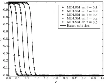
Assuming the velocity eld as V(x; t) = C, the one-dimensional form of Eq. (13) can be used to model the one-dimensional nonlinear wave. The size of the domain is assumed to be equal to one. The quadratic basis function is used to solve this problem. The exact solution to this problem is available as follows:
C(x; t) = f2+ f1eH(x mt)
1 + eH(x mt) ; (32)
where H and m are dened as:
H = 21 (f2 f1); (33)
m = 12(f2+ f1): (34)
f1 and f2 are assumed to be equal to zero and one,
respectively. The exact solution is used to dene the initial and Dirichlet-type boundary conditions. Dier-ent regular nodal distributions are used to solve this problem. A series of tests is also carried out to study the sensitivity of the results to dierent Peclet numbers dened as the dimensionless ratio of the advection term to the diusion term. For this purpose, the problem is solved with a set of dierent diusion coecients leading to high gradient solutions and higher numerical errors.
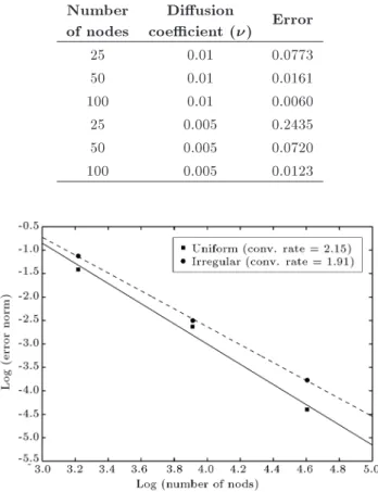
Figures 4 and 5 compare the solutions of the MDLSM method with the exact solutions considering the diusion coecient as = 0:01. The problem is also solved for = 0:005. The results are shown in Figures 6 and 7. In all cases, the ratio of the time step size to the nodal spacing is equal to 0.1.
The time-averaged error of the results is presented in Table 2 to show the sensitivity of the results with respect to the number of nodes and diusion coe-cients. As expected, the results indicate that the error
Figure 4. Comparison of MDLSM results with the exact solutions for 26 nodes and = 0:01 (second example).
Figure 5. Comparison of MDLSM results with the exact solutions for 101 nodes and = 0:01 (second example).
Figure 6. Comparison of MDLSM results with the exact solutions for 26 nodes and = 0:005 (second example).
Figure 7. Comparison of MDLSM results with the exact solutions for 101 nodes and = 0:005 (second example).
Table 2. Sensitivity analysis with respect to the number of nodes and diusion coecient (Peclet number) for one-dimensional wave travel problem.
Number of nodes
Diusion
coecient () Error
25 0.01 0.0773
50 0.01 0.0161
100 0.01 0.0060
25 0.005 0.2435
50 0.005 0.0720
100 0.005 0.0123
Figure 8. Convergence rate for = 0:005 (second example).
is higher for the smaller diusion coecients (higher Peclet number) and the results are more accurate for the ner nodal distributions. A set of non-uniform nodal distributions is used to investigate the eect of non-uniform nodal distribution on the accuracy of results. Figure 8 compares the convergence rates of uniform and non-uniform nodal distributions. Using the 50 nodes for = 0:005, the gradients are computed by the DLSM and MDLSM methods. The error norms of the gradients are 0.0912 and 0.0843 for DLSM and MDLSM methods, respectively, indicating the higher accuracy of the MDLSM.
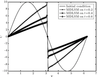
4.3. Burger's one-dimensional equation with periodic boundary conditions
In this section, Burger's non-linear one-dimensional equation V(x; t) = C, is considered with periodic boundary conditions. The size of the domain is considered as 2. The MLS shape functions are produced by the cubic basis function. To impose the periodic boundary conditions, the computational domain is extended at the periodic boundaries and the unknown values at the nodes on the right and left sides of the domain are considered equal [54]. Figure 9 illustrates the schematic view of the process. In this
Figure 9. Repetitive domain and the support domains to impose the periodic boundary conditions.
Figure 10. Comparison of MDLSM results with the analytical solutions for 100 regular nodal distributions and = 1 (third example).
gure, I-th node represents nodal points on the right-and left-hright-and sides of the boundaries. The function C(x; t) = 10 sin(x) is used as the initial condition.
Figure 10 compares the results of the proposed MDLSM method with the available analytical solutions for = 1 [55]. This problem is also solved for dierent values of the diusion coecients = 0:01 and 0.001 using dierent numbers of nodal points distributed uniformly in the domain. The results are shown in Figures 11 to 14. It can be seen that while the results are of high accuracy for the smallest diusion coecient, the accuracy of the results decreases with increase in the value of the diusion coecient. Fur-thermore, Figures 11 and 13 show that with coarse nodal distributions of 100 and 150 nodal points, the method is divergent for = 0:01 and = 0:001, respectively. On the other hand, Figures 12 and 14 indicate that for diusion coecient values of 0.01 and 0.001, uniformed distributions of 150 and 512 nodes are enough to produce convergent and accurate results, respectively.
4.4. Two-dimensional Gaussian hill problem The diusion of a Gaussian hill in a uniformly rotating ow eld controlled by the velocity of V(x; t) = ( !(x2 O2); !(x1 O1)) is solved in this section.
Here, (O1; O2) is the center of domain, x1 and x2 are
Figure 11. Results of the MDLSM for 100 regular nodal distributions and = 0:01 (third example).
Figure 12. Results of the MDLSM for 150 regular nodal distributions and = 0:01 (third example).
Figure 13. Results of the MDLSM for 150 regular nodal distributions and = 0:001 (third example).
Figure 14. Results of MDLSM for 512 regular nodal distributions and = 0:001 (third example).
the rotational velocity. The analytical solution to this problem on an innite plate is dened as follows [56]:
C(x; t) = A0 1 + (2t
2)
exp( ~x21+ ~x22
2(2+ 2t)); (35)
where: ~
x1= (x1 O1) Q1cos !t + Q2sin !t;
and: ~
x2= (x2 O2) Q1sin !t Q2cos !t:
Q1and Q2dene the initials of the Gaussian hill center.
The constant values considered are A0 = 1, 2 = 2,
= 10 5, and ! = 10 6.
The domain of the problem is a square domain measuring 20 20 and (Q1; Q2) = (15; 10). The
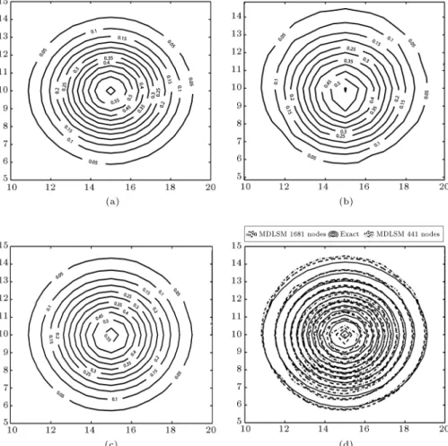
analytical solution is used to impose the initial and Dirichlet boundary conditions. Linear basis function is used and the results are presented after one rotation produced in 2000 time steps. The domain is discretized by two sets of regular nodal distributions of 441 and 1681 nodes. The errors of the MDLSM method for each set of coarse and ne nodal distributions are 0.1113 and 0.0635, respectively. The analytical and numerical results are compared in Figure 15.
4.5. Burger's two-dimensional equation
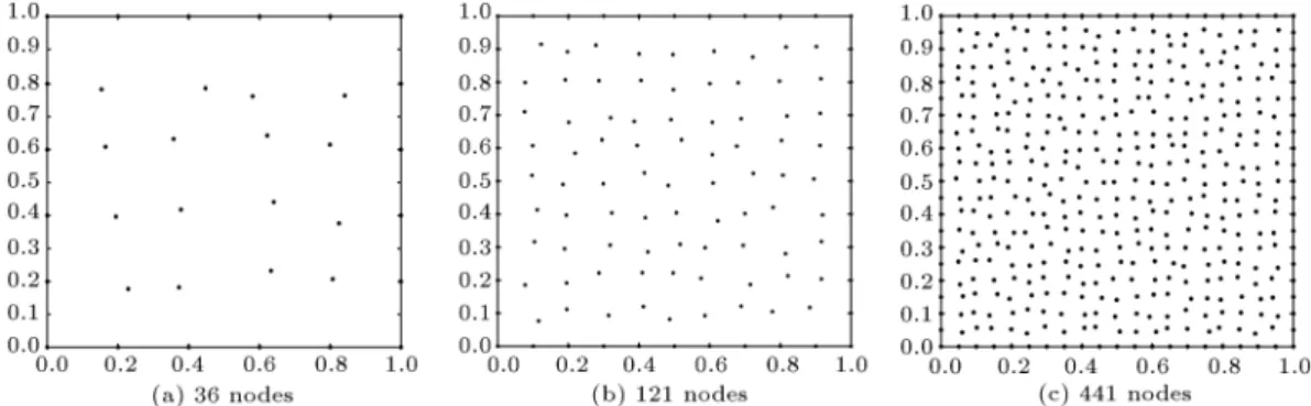
Burger's two-dimensional equation can be represented by taking V(x; t) = C in Eq. (13). The problem is solved in a unit square domain discredited by a regular nodal distribution of 441 nodes. The exact solution to this problem is available as:
C(x; t) = 1 + exp(x + y t 0:25)=(2)1 ; (36) where x and y dene the coordinates and is assumed to be 0.03 in this problem. The exact solution is
Figure 15. Comparison of the contour lines of exact and MDLSM solutions (forth example): (a) Exact solution, (b) MDLSM results obtained for regular distribution of 441 nodes, (c) MDLSM results obtained for regular distribution of 1681 nodes, and (d) all results.
used to impose the Dirichlet boundary conditions. The time step size, t, is equal to 0.001. The penalty coecient is taken as = 104. Figure 16 compares
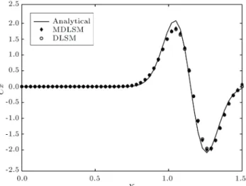
the numerical and the exact results. This comparison shows the high accuracy of the proposed MDLSM method for solving non-linear convection-dominated problems. The problem is also solved with t = 0:01 to investigate the inuence of the penalty parameter, of which the results are demonstrated in Figure 17. The results show that accuracy generally improves by increasing penalty parameter. However, when the penalty exceeds a specied value, the coecient matrix becomes ill-posed and the error sharply increases. A set of irregular nodal distributions, presented in Figure 18, are also used to study the eect of the irregular nodal conguration on the results. The convergence rate of the method is shown in Figure 19 for the results at t = 0:5 s for both uniform and irregular nodal distributions. The gradients of the solutions obtained on a uniform 21 21 nodal distribution are also compared in Figure 20. The obtained results show that the gradients of the solutions are remarkably accurate in MDLSM method compared to DLSM method.
Figure 16. Comparison of MDLSM results with the exact solutions at t = 0:5 and y = 0:5 (fth example).
In Table 3, the CPU times of the DLSM and MDLSM methods are compared. In the MDLSM method, the cumbersome second derivatives of the MLS are not required and, hence, the CPU time of the
Table 3. Comparison of CPU times of the DLSM and MDLSM methods in one time step (fth example). Number of
nodes
MLS (DLSM)
MLS (MDLSM)
Solving procedure (DLSM)
Solving procedure (MDLSM)
36 0.02918 0.01549 0.00041 0.009195
121 0.1171 0.0591 0.01521 0.02476
441 2.3205 0.2417 0.02120 0.24771
Figure 17. Inuence of the penalty factor (fth example).
approximation procedure is less than that of DLSM method. However, the size of the coecient matrix is larger in the MDLSM method and the CPU time of the solving procedure increases compared to the DLSM method. Therefore, the total computational cost is dependent on the type of the problem being solved. When Eulerian type of simulation is considered, the computational cost of the MDLSM method is higher than that of the DLSM method since the MLS shape functions require to be constructed once. However, for the problems with the moving nodes as those encountered in Lagrangian simulation, in which the MLS shape functions need to be constructed for each new nodal position, the computational eort of the MDLSM method would be lower than that of DLSM.
Figure 19. Convergence rate of MDLSM method at t = 0:5 (s) for uniform and irregular nodal distributions (fth example).
5. Conclusion
A truly meshless method, namely, MDLSM, was pre-sented in this paper to solve propagation problems. The method was based on the minimization of the least squares functional with respect to the nodal parameters. The least squares functional was dened as the sum of the squared residuals of the dierential equation and its boundary conditions. The MLS shape function was used to approximate the solutions. The coecient matrix of the MDLSM method is always symmetric positive-denite, circumventing the LBB condition. With the MDLSM method, calculation of second derivatives of shape function was not required and the gradient of solutions was accurately computed
Figure 20. Comparison of the gradients of the DLSM and MDLSM methods at t = 0:5 and y = 0:5 (fth example).
compared with the DLSM method. The eciency and accuracy of the method were evaluated via some numerical examples. The numerical results were pre-sented and compared with the available analytical solutions. The results indicated high eciency of the MDLSM method in solving both linear and non-linear convection-dominant problems. Comparison of the CPU times required by the DLSM and MDLSM methods for the test examples showed that although MDLSM was more expensive than DLSM for problems with xed nodal point positions, it could be cheaper for the problems with moving nodes, i.e. Lagrangian simulations.
References
1. Shao, S. and Lo, E.Y. \Incompressible SPH method for simulating Newtonian and non-Newtonian ows with a free surface", Advances in Water Resources, 26(7), pp. 787-800 (2003).
2. Khanpoura, M., Zarratia, A.R., Kolahdoozana, M., Shakibaeiniab, A., and Amirshahia, S.M. \Mesh-free SPH modeling of sediment scouring and ushing", Computers & Fluids, 129, pp. 67-78 (2016).
3. Chen, Z., Zong, Z., Liu, M.B., Zou, L., Li, H.T., and Shu, C. \An SPH model for multiphase ows with complex interfaces and large density dierences", Journal of Computational Physics, 283, pp. 169-188 (2015).
4. Koshizuka, S. and Oka, Y. \Moving-particle semi-implicit method for fragmentation of incompressible uid", Nuclear Science and Engineering, 123(3), pp. 421-434 (1996).
5. Macia, F., Souto-Iglesias, A., Gonzalez, L.M., and Cercos-Pita, J.L. \<MPS>=<SPH>", 8th Interna-tional SPHERIC Workshop (2013).
6. Ataie-Ashtiani, B. and Farhadi, L. \A stable moving-particle semi-implicit method for free surface ows", Fluid Dynamics Research, 38(4), pp. 241-256 (2006).
7. Sun, Z., Djidjeli, K., Xing, J.T., and Cheng, F. \Coupled MPS-modal superposition method for 2D nonlinear uid-structure interaction problems with free surface", Journal of Fluids and Structures, 61, pp. 295-323 (2016).
8. Shakibaeinia, A. and Jin, Y.-C. \MPS mesh-free par-ticle method for multiphase ows", Computer Methods in Applied Mechanics and Engineering, 229, pp. 13-26 (2012).
9. Kolahdoozan, M., Ahadi, M., and Shirazpoor, S. \Eect of turbulence closure models on the accuracy of moving particle semi-implicit method for the viscous free surface ow", Scientia Iranica. Transactions A, Civil Engineering, 21(4), p. 1217 (2014).
10. Monaghan, J., Kos, A. and Issa, N. \Fluid motion generated by impact", Journal of Waterway, Port, Coastal, and Ocean Engineering, 129(6), pp. 250-259 (2003).
11. Shakibaeinia, A. and Jin, Y.C. \A weakly compressible MPS method for modeling of open-boundary free-surface ow", International Journal for Numerical Methods in Fluids, 63(10), pp. 1208-1232 (2010). 12. Khayyer, A. and Gotoh, H. \Modied moving particle
semi-implicit methods for the prediction of 2D wave impact pressure", Coastal Engineering, 56(4), pp. 419-440 (2009).
13. Liu, C.-S. and Young, D. \A multiple-scale Pascal polynomial for 2D stokes and inverse Cauchy-Stokes problems", Journal of Computational Physics, 312, pp. 1-13 (2016).
14. Liu, C.-S. \Homogenized functions to recover H(t)=H(x) by solving a small scale linear system of dierencing equations", International Journal of Heat and Mass Transfer, 101, pp. 1103-1110 (2016). 15. Belytschko, T., Lu, Y.Y., and Gu, L. \Element-free
Galerkin methods", International Journal for Numer-ical Methods in Engineering, 37(2), pp. 229-256 (1994). 16. Liu, L., Chua, L., and Ghista, D. \Element-free Galerkin method for static and dynamic analysis of spatial shell structures", Journal of Sound and Vibra-tion, 295(1), pp. 388-406 (2006)
17. Deng, Y., Liu, C., Peng, M., and Cheng, Y. \The interpolating complex variable element-free Galerkin method for temperature eld problems", International Journal of Applied Mechanics, 7(02), p. 1550017 (2015).
18. Zhang, Z., Liew, K.M., Cheng, Y., and Lee, Y.Y. \Analyzing 2D fracture problems with the improved element-free Galerkin method", Engineering Analysis with Boundary Elements, 32(3), pp. 241-250 (2008). 19. Singh, A., Singh, I.V., and Prakash, R. \Meshless
element free Galerkin method for unsteady nonlinear heat transfer problems", International Journal of Heat and Mass Transfer, 50(5), pp. 1212-1219 (2007). 20. Belytschko, T., Gu, L., and Lu, Y. \Fracture and crack
growth by element free Galerkin methods", Modelling and Simulation in Materials Science and Engineering, 2(3A), p. 519 (1994).
21. Atluri, S. and Zhu, T. \A new meshless local Petrov-Galerkin (MLPG) approach in computational mechan-ics", Computational Mechanics, 22(2), pp. 117-127 (1998).
22. Atluri, S., Liu, H., and Han, Z. \Meshless local Petrov-Galerkin (MLPG) mixed nite dierence method for solid mechanics", Computer Modeling in Engineering and Sciences, 15(1), p. 1 (2006).
23. Enjilela, V. and Arefmanesh, A. \Two-step Taylor-characteristic-based MLPG method for uid ow and heat transfer applications", Engineering Analysis with Boundary Elements, 51, pp. 174-190 (2015).
24. Luan, T. and Sun, Y. \Solving a scattering problem in near eld optics by a least-squares method", Engineer-ing Analysis with Boundary Elements, 65, pp. 101-111 (2016).
25. Arzani, H. and Afshar, M. \Solving Poisson's equations by the discrete least square meshless method", WIT Transactions on Modelling and Simulation, 42, pp. 23-31 (2006).
26. Firoozjaee, A.R. and Afshar, M.H. \Discrete least squares meshless method with sampling points for the solution of elliptic partial dierential equations", Engineering Analysis with Boundary Elements, 33(1), pp. 83-92 (2009).
27. Afshar, M., Lashckarbolok, M., and Shobeyri, G. \Collocated discrete least squares meshless (CDLSM) method for the solution of transient and steady-state hyperbolic problems", International Journal for Numerical Methods in Fluids, 60(10), pp. 1055-1078 (2009).
28. Afshar, M. and Lashckarbolok, M. \Collocated discrete least-squares (CDLS) meshless method: Error esti-mate and adaptive renement", International Journal for Numerical Methods in Fluids, 56(10), pp. 1909-1928 (2008).
29. Afshar, M., Amani, J., and Naisipour, M. \A node en-richment adaptive renement in discrete least squares meshless method for solution of elasticity problems", Engineering Analysis with Boundary Elements, 36(3), pp. 385-393 (2012).
30. Kazeroni, S.N. and Afshar, M. \An adaptive node regeneration technique for the ecient solution of elas-ticity problems using MDLSM method", Engineering Analysis with Boundary Elements, 50, pp. 198-211 (2015).
31. Shobeyri, G. and Afshar, M. \Simulating free sur-face problems using discrete least squares meshless method", Computers & Fluids, 39(3), pp. 461-470 (2010)
32. Shobeyri, G. and Afshar, M. \Adaptive simulation of free surface ows with discrete least squares meshless (DLSM) method using a posteriori error estimator", Engineering Computations, 29(8), pp. 794-813 (2012)
33. Pehlivanov, A., Carey, G., and Lazarov, R. \Least-squares mixed nite elements for second-order elliptic problems", SIAM Journal on Numerical Analysis, 31(5), pp. 1368-1377 (1994).
34. Jiang, B.-N., Lin, T., and Povinelli, L.A. \Large-scale computation of incompressible viscous ow by least-squares nite element method", Computer Methods in Applied Mechanics and Engineering, 114(3), pp. 213-231 (1994).
35. Faraji, S., Afshar, M., and Amani, J. \Mixed discrete least square meshless method for solution of quadratic partial dierential equations", Scientia Iranica, 21(3), pp. 492-504 (2014).
36. Amani, J., Afshar, M., and Naisipour, M. \Mixed discrete least squares meshless method for planar elasticity problems using regular and irregular nodal distributions", Engineering Analysis with Boundary Elements, 36(5), pp. 894-902 (2012).
37. Kumar, R., A Least-Squares/Galerkin Split Finite Element Method for Incompressible and Compressible Navier-Stokes Equations, ProQuest (2008).
38. Shcherbakov, V. and Larsson, E. \Radial basis func-tion partifunc-tion of unity methods for pricing vanilla basket options", Computers & Mathematics with Ap-plications, 71(1), pp. 185-200 (2016).
39. Hon, Y.-C., Sarler, B., and Yun, D.-f. \Local radial basis function collocation method for solving thermo-driven uid-ow problems with free surface", Engi-neering Analysis with Boundary Elements, 57, pp. 2-8 (2015).
40. Dehghan, M. and Abbaszadeh, M. \Two meshless pro-cedures: moving Kriging interpolation and element-free Galerkin for fractional PDEs", Applicable Analy-sis, pp. 1-34 (2016).
41. Peco, C., Millan, D., Rosolen, A., and Arroyo, M. \Ef-cient implementation of Galerkin meshfree methods for large-scale problems with an emphasis on maximum entropy approximants", Computers & Structures, 150, pp. 52-62 (2015).
42. Arroyo, M. and Ortiz, M. \Local maximum-entropy approximation schemes: a seamless bridge between nite elements and meshfree methods", Interna-tional Journal for Numerical Methods in Engineering, 65(13), pp. 2167-2202 (2006)
43. Wang, J. and Liu, G. \Radial point interpolation method for elastoplastic problems", ICSSD 2000, 1st Structural Conference on Structural Stability and Dy-namics (2000).
44. Tanaka, Y., Watanabe, S., and Oko, T. \Study of eddy current analysis by a meshless method using RPIM", IEEE Transactions on Magnetics, 51(3), pp. 1-4 (2015).
45. Liu, G.-R., Meshfree Methods: Moving Beyond the Finite Element Method, CRC press (2009).
46. Li, X. and Zhang, S. \Meshless analysis and applica-tions of a symmetric improved Galerkin boundary node
method using the improved moving least-square ap-proximation", Applied Mathematical Modelling, 40(4), pp. 2875-2896 (2016)
47. Li, X. \A meshless interpolating Galerkin boundary node method for Stokes ows", Engineering Analysis with Boundary Elements, 51, pp. 112-122 (2015) 48. Li, X. \Meshless Galerkin algorithms for boundary
integral equations with moving least square approxi-mations", Applied Numerical Mathematics, 61(12), pp. 1237-1256 (2011).
49. Li, X. \Error estimates for the moving least-square approximation and the element-free Galerkin method in n-dimensional spaces", Applied Numerical Mathe-matics, 99, pp. 77-97 (2016).
50. Liu, G.-R. and Gu, Y.-T., An Introduction to Meshfree Methods and Their Programming, Springer Science & Business Media (2005).
51. Li, X., Zhang, S., Wang, Y., and Chen, H. \Analysis and application of the element-free Galerkin method for nonlinear sine-Gordon and generalized sinh-Gordon equations", Computers & Mathematics with Applica-tions, 71(8), pp. 1655-1678 (2016)
52. Li, X., Chen, H., and Wang, Y. \Error analysis in Sobolev spaces for the improved moving least-square approximation and the improved element-free Galerkin method", Applied Mathematics and Compu-tation, 262, pp. 56-78 (2015)
53. Van de Vosse, F. and Minev, P. \Spectral elements methods: Theory and applications", EUT Report, 96-W-001 ISBN 90-236-0318-5, Eindhoven University of Technology (1996).
54. Coppoli, E.H.R., Mesquita, R.C., and Silva, R.S. \Periodic boundary conditions in element free Galerkin method", COMPEL-The International Journal for Computation and Mathematics in Electrical and Elec-tronic Engineering, 28(4), pp. 922-934 (2009). 55. Moin, P., Fundamentals of Engineering Numerical
Analysis, Cambridge University Press (2010).
56. Chen, S., Wu, X., Wang, Y., and Kong, W. \High ac-curacy time and space transform method for advection-diusion equation in an unbounded domain", Inter-national Journal for Numerical Methods in Fluids, 58(11), pp. 1287-1298 (2008).
Biographies
Saeb Faraji Gargari received his BSc degree form the Department of Civil Engineering at Urmia University and his MSc degree in Structural and Hydraulic Engi-neering from Iran University of Science and Technology. He is now PhD student at Amirkabir University of Technology. His research interests include improving and developing the mesh-free numerical methods for solving the Partial Dierential Equations (PDEs) gov-erning the engineering problems.
Morteza Kolahdoozan received his BSc degree from the Department of Civil Engineering at Amirkabir Uni-versity of Technology, MSc degree from the Department of Civil Engineering at Tehran University, and PhD degree from the University of Bradford, UK. He is Associate Professor in the Department of Civil and Environmental Engineering at Amirkabir University of Technology, Tehran, Iran. His research interests include numerical and physical simulation of the uid mechanics problems. The emphasis of his researches is on coastal hydrodynamics, sediment transport, and oil propagation.
Mohammad Hadi Afshar obtained his BSc degree in Civil Engineering from Tehran University, and MSc and PhD degrees from University College of Swansea. He is now Associate Professor in Civil Engineering Department at Iran University of Science and Technol-ogy. His research interests include numerical modeling of elasticity and uid mechanics problems, especially using the mesh-free methods and optimization.