Sharif University of Technology
Scientia IranicaTransactions A: Civil Engineering http://scientiairanica.sharif.edu
A new method for three-dimensional stability analysis
of earth slopes
M. Hajiazizi
a;, P. Kilanehei
a, and F. Kilanehei
ba. Department of Civil Engineering, Razi University, Taq-e Bostan, Kermanshah, P.O. Box 67149-67346, Iran. b. Department of Civil Engineering, Imam Khomeini International University, Qazvin, P.O. Box 34148-96818, Iran. Received 15 December 2015; received in revised form 19 May 2016; accepted 8 October 2016
KEYWORDS Limit equilibrium; Factor of safety; 3D analysis; Earth slope; 3D slice.
Abstract. In this research, a new three-dimensional limit equilibrium method was developed. In the proposed method, the slip surface was assumed to be spherical and slices were assumed along the slip surface radius converging to a point. Moreover, force and moment equilibrium equations were used. In order to calculate Factor of Safety (FS) with the proposed method, a code was developed for two- and three-dimensional states. The model used the iteration (trial and error) method to simultaneously satisfy force and moment equilibrium equations. In order to ensure convergence of the numerical model developed in the three-dimensional state, the under-relaxation method was used in the trial and error operations. In examples, the value of FS obtained by the proposed method was 2.5 to 12 percent higher than those obtained by the other methods. In order to validate the proposed method and assess the functionality of the three-dimensional numerical model, a few examples were solved under dierent circumstances; the results were properly compliant with the results of other methods.
© 2018 Sharif University of Technology. All rights reserved.
1. Introduction
Stability analysis of earth slopes is an important concern in civil engineering and one of the substantial concerns in the design of earth slopes, routes, canals, and embankments. Slope stability analysis is the process of controlling the safety of a natural or articial slope [1]. The slope might be the result of excavation or embanking. The control involves calculation of shear stresses occurring along the most critical and probable slip surface and comparison of the shear stress values with the shear strength of soil. Finding the critical slip surface of slopes and calculating the FS corresponding to this surface are two of the fundamental concerns in
*. Corresponding author. Tel./Fax: +98 83 34283264 E-mail addresses: [email protected] (M. Hajiazizi); [email protected] (P. Kilanehei); [email protected] (F. Kilanehei) doi: 10.24200/sci.2017.4173
the stability analysis of earth slopes. It is important to nd the most critical slip surface because calculation of the minimum FS, which is obtained at this surface, is usually the objective of stability analysis. Limit Equilibrium (LE) methods are among the oldest means of determining critical slip surfaces and the minimum FS. In the LE methods, FS is calculated by assuming a failure surface and satisfying the static equilibrium equations for that surface. Moreover, in these methods, the number of equilibrium equations is lower than the number of unknowns and, therefore, usually additional hypotheses are required to turn the problem at hand into a determinate one.
In the Fellenius method [2], the inter-slice forces were neglected and FS was calculated based on the moment equilibrium around the center of the failure surface. In the Bishop method [3], FS was calculated by assuming a circular failure surface and satisfaction of moment and vertical force equilibrium equations. The methods by Lowe and Karaath [4] and the
modied Janbu method [5] as well as US Army Corps of Engineers [6] also calculated FS by satisfying the force equilibrium equations. The dierence between dierent methods, which obtain FS by satisfying the force equilibrium equations, lies in their hypotheses for the angle of the forces between the slices. Therefore, every method considers dierent force angles. The methods by Spencer [7], Morgenstern and Price [8], and Sarma [9] calculated FS based on a few hypotheses and satisfaction of the force and moment equilibrium equations. Cheng [10] calculated FS using the double QR method and indicated that the new method per-formed better in converging the results. Cheng and Zhu [11] proposed a single relation for two-dimensional calculation of FS using the LE method. In addition, in order to calculate FS, they used the Gauss-Newton linear approximation. Zhu et al. [12] proposed a simple algorithm for calculating FS using the Morgenstern and Price method [8]. In this algorithm, the initial values of FS and the scale factor were used in an iterative process to calculate the converged FS and . Hajiazizi and Mazaheri [13] presented the line segments slip surface for optimized design of piles in stabilization of the earth slopes using limit equilibrium method for calculating FS. Xiao et al. [14] combined the numerical method and LE method to dene the critical failure surface for earth slopes. In their method, numerical analysis was used to determine the assumptive failure surface and the LE method was used to calculate FS. Deng and Li used radiation slices method for arbitrary curved slip surface in 2D state [15].
Hajiazizi and Tavana [16] used the TDAVLG optimization method and LE method to calculate the minimum FS corresponding to the non-spherical slip surface in three dimensions. Cheng et al. [17] used the LE method for stability analysis of slopes and faced a convergence problem. In order to solve that problem, they proposed a simple method and assessed it. Stability analysis of earth slopes mainly takes place in two dimensions by assuming a planar strain. However, in many cases, three-dimensional analysis is necessary as a two-dimensional analysis would be unrealistic. These cases usually include slopes under concentrated loads, slopes with small length to height ratios, and slopes with curved plans. Three-dimensional stability analyses of slopes, which have been carried out rarely, are mostly based on the LE method. Many of the three-dimensional analysis methods were proposed by extending two-dimensional methods to the dimensional space. The three-dimensional method by Hovland [18] was an exten-sion of the simple slice method, which was a two-dimensional method. Hungr [19] also proposed a three-dimensional analysis method, which was a direct ex-tension of the hypotheses used in the simplied Bishop method. The three-dimensional method by Ugai and
Hosobori [20] was also an extension of Spencer's two-dimensional method [7], which calculated the three-dimensional FS using the force-moment equilibrium. Cheng and Lau [21] proposed the asymmetric slope stability models based on extensions of the Bishop [3], Janbu [5], and Morgenstern-Price methods [8] in three dimensions. Much progress has been attained in 2D and 3D methods of stability of slopes in recent years [22-24]. Zhou and Cheng [25] presented the rigor-ous limit equilibrium column method, in which inter-column forces were taken into account based on six equilibrium conditions, which included three direction force equilibrium conditions along coordinate axes and three direction moment equilibrium conditions around three coordinate axes. Zhu and Qian [26] presented the rigorous and quasi-rigorous limit equilibrium solutions to 3D slope stability, which satised six and ve equilibrium conditions. Cheng and Zhou [27] presented a novel displacement-based rigorous limit equilibrium method to investigate the displacements and stabilities of three-dimensional landslides. Zhou and Cheng [28] presented a novel displacement-based rigorous limit equilibrium method to analyze the stability and the dis-placement of three-dimensional (3D) creeping slopes.
Three-dimensional slip surfaces are closer to real-ity than two-dimensional slip surfaces. Failure surfaces are usually spherical in homogeneous clay soils. In this paper, a new limit equilibrium method has been proposed for these surfaces. Although in multi-layered soils, consideration of spherical slip surface is a simpli-fying assumption, in homogeneous clay soils, it can be a reasonable assumption. It is noteworthy that in multi-layered slopes, failure surface is non-aspherical, which is studied in [16]. In soils with zero internal friction angle, slip surface is circular in two-dimensional space and spherical in three-dimensional space [29].
According to the relations proposed by the afore-mentioned methods, direction of slip is similarly ob-tained in all methods based on the force-moment equilibrium in three dimensions. In this research, all of the forces acting on slices are calculated in the three-dimensional state using the LE method based on given slice shapes. The moment-force equilibrium equations are also applied. Afterwards, after satisfying the equilibrium equations (moment and force equilibrium), FS is calculated more precisely and it is shown that the result is larger than the results of other LE methods.
The considered assumptions are as follows:
(i) Morgenstern-Price equation is valid;
(ii) Forces are applied at the center of slices surfaces. 2. Limit equilibrium equations for the method
proposed for two dimensions
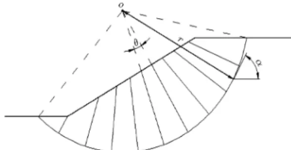
Figure 1. The slip wedge in an earth slope.
Figure 2. The free diagram for forces acting in one slice. two dimensions. The slip wedge is divided into several slices along the semi-diameter. Figure 2 shows the free diagram for forces acting on a slice. The forces include the slice weight (Wi), inter-slice forces (including the
shear component, Xi, and the normal component, Ei),
shear strength (Si), and normal force (Ni) that act
on the slice oor. By writing the force equilibrium equations along the Xi+1 and Ei+1 directions and
satisfying the moment equilibrium conditions around the failure surface center (point o), it is possible to obtain the force-moment equilibrium equations. 2.1. Force equilibrium equations
Eqs. (1) and (2) are obtained based on Figure 2 and the force equilibrium equations that were written along the Xi+1 and Ei+1 directions:
Xi+1+ W cos (/i =2) N cos =2 S sin =2
+ Eisin Xicos = 0; (1)
Ei+1 W sin (i =2) N sin =2 + S cos =2
Eicos Xisin = 0; (2)
where w is weight of slice and Xi, Xi+1, Ei, Ei+1, S,
and N are forces acting on a slice (Figure 2).
By multiplying the expression on both sides of Eqs. (1) and (2) by cos =2 and sin =2, Eqs. (3) and (4) are, respectively, obtained:
Xi+1cos =2 + W cos (i =2) cos =2
N cos2=2 S sin =2 cos =2
+ Eisin cos =2 Xicos cos =2 = 0; (3)
Ei+1sin =2 W sin (i =2) sin =2
N sin2=2 + S cos =2 sin =2
Eicos sin =2 Xisin sin =2 = 0: (4)
By summing up Eqs. (3) and (4), it is possible to calculate the N force as follows:
N =Xi+1cos =2 + Ei+1sin =2 + W cos i
+ Eisin =2 Xicos =2: (5)
Shear strength S is calculated by multiplying both sides of Eqs. (1) and (2) by sin =2 and cos =2:
Xi+1sin =2 + W s (i =2) sin =2
N cos =2 sin =2 S sin2=2
+ Eisin sin =2 Xicos sin =2 = 0; (6)
Ei+1cos =2 + W sin (i =2) cos =2
+ N sin =2 cos =2 S cos2=2
+ Eicos cos =2 + Xisin cos =2 = 0: (7)
By summing up Eqs. (6) and (7), Eq. (8) is obtained: S =Xi+1sin =2 Ei+1cos =2 + Xisin =2
+ Eicos =2 + W sin i: (8)
On the other hand, Eq. (8) is rewritten as Eq. (10) based on Eq. (9):
S = F1 (C0L + (N UL) tan '0) ; (9)
Xi+1sin =2 Ei+1cos =2 + Xisin =2
+ Eicos =2 + W sin i C 0L
F tan '0
F (Xi+1cos =2 + Ei+1sin =2 + W cos i+ Eisin =2 Xicos =2)
Ei+1=
C0L
F ULF tan '0+ W
tan '0
F cos i sin i f(x)sin =2 cos =2 tan 'F 0 f(x)cos =2 + sin =2
+
f(x)sin =2 cos =2 +tan '
0
F sin =2 f(x)cos =2
Ei
f(x)sin =2 cos =2 tan 'F 0 f(x)cos =2 + sin =2 : (11)
Box I
where FS is safety factor, and C0 and 0 are eective
cohesion and eective friction angle of soil, respectively. U is the pore water pressure and L the length of each slice oor. The force equilibrium equation is obtained by Eq. (11) as shown in Box I, where i is the angle
of each slice oor to the horizontal line while f(x) is a hypothetical function showing the relationship between the normal and shear forces in each slice. is the scale factor and shows the central angle in each slice. Concerning Eq. (11), which was obtained based on the force equilibrium, the following points shall be taken into account:
1. There are two unknowns in Eq. (11), namely, the factor of safety and the scale factor ();
2. The inter-slice force (Ei+1) in each phase depends
on the inter-slice force (Ei) in the previous step
(recursive relation);
3. The boundary conditions for the equation are Ei=
0 and Ei+1= 0 because there is no slice before the
rst slice and after the last one.
In order to obtain the moment equilibrium equa-tion, rst, the shear strength relation is calculated based on inter-slice forces. Next, by satisfying the moment equilibrium around the failure surface center, the moment equilibrium relation is obtained. The shear strength relation is also expressed as follows based on the inter-slice forces:
N =Ei+1 sin =2 + f(x)cos =2
+ Ei sin =2 f(x)cos =2+ W cos i; (12)
S =F1 C0L +E
i+1 sin =2 + f(x)cos =2
+ Ei sin =2 f(x)cos =2+ W cos i
ULtan '0: (13)
The moment equilibrium equation is also written as follows:
X
Wisin ii Sr = 0: (14)
By putting Si into Eq. (14) and simplifying the
equa-tion, it is possible to achieve the moment equilibrium equation as shown in Box II, where, r is the failure semi-diameter and is the moment arm in each slice. 2.2. Calculation of FS in two dimensions Eqs. (11) and (15) are the basic equations resulting from the force and moment equilibrium equations. Simultaneous satisfaction of these equations leads to FS. In this research, FS was calculated using the iterative method and it was obtained by satisfying the force and moment equilibrium equations. Methods that satisfy all equilibrium equations and employ fewer simplifying assumptions lead to low errors compared to other methods. Hence, Eqs. (11) and (15) are expected to determine FS more precisely.
2.3. Developing a numerical model for calculation of FS
In order to calculate FS with the method proposed in this research, a code was developed in FORTRAN. In this model, the specications of the earth slope (including the slope geometry, soil resistance proper-ties, and water level) are taken as inputs. Next, the
F = P
C0Lr + sin =2 + f
(x)cos =2Ei+1r tan '0 P
(Wisin ii) +
P
sin =2 f(x)cos =2P Ei+ W cos i ULr tan '0
(Wisin ii) : (15)
slip wedge is introduced and based on the number of divisions dened by the user, the slip wedge is sliced. Afterwards, the coordinates of each node on these slices are determined. After determining the coordinates of nodes on each slice, it is possible to calculate the area, weight, the oor-horizon angle, surface center, moment arm, and pore water pressure on each slice.
Based on the coordinates of all slices, it is then possible to calculate FS. In order to calculate FS, it is necessary to go through a process that simultane-ously satises force and moment equilibrium equations (Eqs. (11) and (15)). Therefore, the force equilibrium equation is satised using an initial FS. To this end, the inter-slice forces acting on other slices are calculated using a scale factor and a zero inter-slice force for the rst slice (E1 = 0). When the inter-slice force
acting on the last slice is zero, the force equilibrium equation is satised; otherwise, changes in order for the last boundary condition (En+1 0) to be
met. By putting and inter-slice forces resulting from satisfaction of the force equilibrium into the moment equilibrium equation, it is possible to calculate the FS resulting from the moment equation.
If the dierence between the initial FS and the FS resulting from the moment equilibrium is slight (smaller than 10 4), the resulting FS is acceptable;
otherwise, the initial FS is replaced by the FS resulting from the moment equilibrium and the previous process is iterated until the dierence between the two consec-utive FS values becomes slight. This way the nal FS is obtained.
3. Three-dimensional limit equilibrium equations in the proposed method
Figure 3 shows a three-dimensional spherical slip sur-face. In order to divide this slip surface into several slices, the slip wedge is divided into sectors with equal
Figure 3. Three-dimensional spherical slip surface.
Figure 4. The free diagram of forces acting in a three-dimensional slice.
intervals. By sectoring the slip surface along the radius, it is possible to calculate the coordinates of points on each slice. Figure 4 shows the free diagram of forces acting on a three-dimensional slice.
In this research, in order to obtain the three-dimensional equilibrium equations, the following hy-potheses were developed:
1. The soil was homogenous;
2. The Mohr-Coulomb failure criterion was valid;
3. The three-dimensional failure surface was spherical;
4. All of the slices moved in one direction.
Based on these hypotheses and Figure 4, the limit equilibrium equations for the three-dimensional state were written.
3.1. Force equilibrium equations
Based on Figure 4 and forces applied to each slice, the force equilibrium equations are written through Eqs. (16) to (18) along the x, y, and z directions:
Smcos x+ N cos x Exicos xi+ Exi+1cos xi+1
Xxi+1sin xi+1+ Xxisin xi= 0; (16)
N cos y Eyicos yi+ Eyi+1cos yi+1
+ Xyisin yi Xyi+1sin yi+1= 0; (17)
Xxi+1cos xi+1 Xxicos xi)
+ (Xyi+1cos yi+1 Xyicos yi)
+ (Eyi+1sin yi+1 Eyisin yi)
W + N cos z+ Smsin x= 0; (18)
where forces of Sm, N, Exi; Exi+1, Xyi, and Xyi+1
are shown in Figure 4. By putting the Mohr-Coulomb relation into Eqs. (16) to (18) and simplifying the equations the force equilibrium equations along the x, y and z axes were obtained by Eqs. (19) to (21):
Exi+1cos xi+1 Exicos xi
= x(Exi+1sin xi+1 Exisin xi)
N cos x cos F x(c0A + (N U) tan '0) ;
(19) Eyi+1cos yi+1 Eyicos yi
=y(Eyi+1sin yi+1 Eyisin yi) N cos y;
(20)
N = 1
cos z+tan '0Fsin x
" W
x(Exi+1cos xi+1 Exicos xi)
y(Eyi+1cos yi+1 Eyicos yi)
(Exi+1sin xi+1 Exisin xi)
(Eyi+1sin yi+1 Eyisin yi)
Ac0sin x
F +
U tan '0
F sin x #
= 0; (21) where A is the area of the slice bottom and N is the force acting on the slice bottom.
As seen in Eq. (21), N (force) is a function of FS. In order to determine N, the FS of the moment equilibrium is put into Eq. (21) provided that the moment equilibrium is required. However, if the force equilibrium is required, the FS of the force equilibrium is put into Eq. (21).
3.2. Force equilibrium along the slip direction In order to obtain the FS equation, a single slip mechanism was assumed in which the paths for all slices were dened along one direction. Hence, in this method, FS of the force equilibrium is calculated by writing the force equation along the x direction:
X
Smcos x+ N cos x= 0: (22)
By putting the Mohr-Coulomb relation into Eq. (22), the FS equation, which results from the force
equilib-rium, is obtained as follows: Ff =
P
(c0A + (N U) tan '0) cos x
P
N cos x : (23)
By calculating the moments of all the slices around a rotation axis, that is parallel to the y-axis and passes through the center of the sphere, the relation for the FS resulting from the moment equilibrium (FSm) is obtained. According to Figure 4, the moment
equilibrium equation is written as follows: X
W disw Smcos xdisz Smsin xdisx
N cos xdisz N cos zdisx = 0; (24)
where disw is the distance between the weight force and the rotation axis, disx is the horizontal distance to rotation axis, and disz is the vertical distance to rotation axis.
Moreover, by putting the Mohr-Coulomb relation into Eq. (24), the relation for calculation of the FS resulting from the moment equilibrium is turned into Eq. (25):
Fm=
P
[c0A+(N U) tan '0](cos xdisz+sin xdisx)
P
W disw N cos xdisz N cos zdisx (25):
Examination of equations for calculation of the FS resulting from the force and moment equilibrium (Eqs. (23) and (25)) indicates that these equations are nonlinear. Moreover, the sum of inter-slice forces (E) can be calculated using equations for calculation of FS. The sum of these forces has to be almost equal to zero. 3.3. Three-dimensional calculation of FS The three-dimensional method proposed in this ar-ticle is an extension of the two-dimensional method and is obtained based on the minimum simplifying assumptions, comprehensible concepts, and adequate precision. In order to calculate FS, the simultaneous satisfaction of force and moment equilibrium equations was employed. Eqs. (23) and (25) are basic equations resulting from the force and moment equilibrium. Therefore, simultaneous satisfaction of these equations results in the required FS. In this case, in order to calculate FS, the iterative method is used and FS is obtained by satisfying the force and moment equilibrium equations.
3.4. Developing a numerical model for 3D calculation of FS
In order to calculate FS using the method proposed in this research, a numerical model was developed in FORTRAN. In this model, the specications of the earth slope (including the slope geometry and soil resistance properties) are taken as inputs. Next, the
radius of the sphere is set by the user and the soil sliding mass is obtained. In the next step, based on the number of divisions dened by the user, the slip wedge is classied and the coordinates of each node on these slices are also determined.
After determining the coordinates of nodes on each slice, it is possible to calculate the following parameters for each slice: volume, area, weight, the oor-horizon angle, the location for application of the normal force and its angle to the axes, angle of inter-slice normal forces to the horizon, and moment arm. In order to calculate the FS resulting from the force and moment equilibrium equations, it is necessary to estimate the initial FS and inter-slice forces.
Afterwards, by averaging the resulting factors of safety for dierent slices, the initial FS for the three-dimensional state is estimated. Moreover, the inter-slice forces calculated in the two-dimensional state are used as the basis for the three-dimensional estimation. In order to calculate FS, it is necessary to go through a process that simultaneously satises force and moment equilibrium equations (Eqs. (23) and (25)). To this end, using the inter-slice forces and the initial FS, and by assuming initial x and y values, normal forces acting on each slice are calculated using Eq. (21). Next, using Eq. (25), the FS resulting from the moment equilibrium is obtained. Next, the force equilibrium equations along the x and y directions (Eqs. (19) and (20)), the values of forces perpendicular to the slip surface in each slice, and the FS resulting from the previous phase are used to calculate the new inter-slice forces. In the next stage, the under-relaxation method is implemented to avoid non-convergence. If the dierence between the new inter-slice force and the initial inter-slice force is large, a percentage of the dierence between these two forces is added to the initial force and the resulting force is used as the new inter-slice force.
This process is iterated until the FS resulting from the moment equilibrium reaches convergence. In the next phases, this process is iterated to determine the FS of the force equilibrium. If the dierence between the resulting factors of safety is slight, the nal FS is calculated; otherwise, values of x and y are changed and the process is repeated until the dierence between the factors of safety resulting from the force and moment equilibrium equations becomes slight. 4. Three-dimensional limit equilibrium and
numerical methods
Three-dimensional limit equilibrium methods and three-dimensional numerical methods, such as nite element method, are located in two dierent categories. Numerical methods, due to their punctuated equilib-rium nature, are more accurate than limit equilibequilib-rium
methods. Slice equilibrium is considered in limit equilibrium methods.
In the limit equilibrium analysis, equilibrium may be considered either for a single free body or for individual vertical slices. Depending on the analysis procedure, complete static equilibrium may or may not be satised. Some assumptions must be made to obtain a statically determinate solution for the factor of safety. Dierent procedures make dierent assumptions, even when they may satisfy the same equilibrium equations. The factor of safety is dened with respect to shear strength and it is computed for an assumed slip surface. In the limit equilibrium analysis, it is necessary to make sucient assumptions regarding the stress distribution along the failure surface such that an overall equation of equilibrium, in terms of stress resultants, may be written for a given problem. Therefore, this simplied approach makes it possible to solve various problems by simple statics [30].
5. Some examples
In this section, in order to examine the proposed method in the two- and three-dimensional states, six examples with dierent conditions are provided. Re-sults of these examples are also analyzed and compared with the results reported by other researchers.
5.1. Example 1
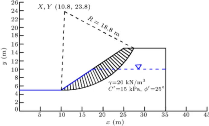
In this example, an earth slope with a height of 10 meters and a 3 to 2 slope ratio (Figure 5) is studied. The slope has the unit weight, cohesion, and angle of friction of 20 kN/m3, 15 kPa, and 25 degrees,
re-spectively. Coordinates of the slip circle center and its radius are Xc= 10:8 m, Yc= 23:8 m, and r = 18:8 m,
respectively. The groundwater level is assumed to be 10 meters. The FS resulting from the proposed method and its comparison with the results of other methods are presented in Table 1. In this example, the lowest FS results from the Fellenius relation by satisfying the moment equilibrium equation and overlooking
inter-Figure 5. An earth slope with a height of 10 meters and a 3 to 2 slope ratio (Examples 1 and 2).
Table 1. Comparison of the safety factor obtained by the proposed method and those by other methods in Example 1. Fellenius [2] Bishop [3] Janbu [5] Morgenstern-Price [8] Proposed method
1.12 1.22 1.14 1.22 1.25
slice shear forces. The FS from the proposed method is larger than the FS from other methods and it is closest to the result of the Morgenstern-Price relation. The proposed method is more reliable than other methods as it represents fewer simplifying assumptions. The fewer simplifying assumptions lead to low errors compared to other methods.
5.2. Example 2
In this example, the rst example without groundwater is solved for the pseudo-dynamic state with a horizontal acceleration of ah = 0:1 g. Results of the FS from
the proposed method and other methods are shown in Table 2. The presence of the earthquake force has reduced FS and increased the instability of the earth slope. These changes can be ascribed to the growth of the driving forces resulting from seismic forces. In this state, the FS resulting from the proposed method is also similar to the results of the modied Bishop and Morgenstern-Price relations [8]. Moreover, Janbu [5] and Fellenius [2] relations also yield the lowest factors of safety.
The proposed method is more reliable than other methods as it represents fewer simplifying assumptions. The fewer simplifying assumptions lead to low errors compared to other methods.
5.3. Example 3
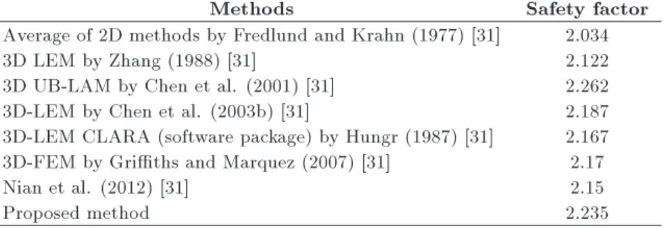
This example is analyzed in [31]. Table 3 presents the results of the method proposed in [31] and methods developed by other researchers for stability analysis of the earth slope in Figure 6. The slope in this gure lacks the weak layer and groundwater param-eters. Using the three-dimensional numerical model developed in this research, the FS for the slope shown in Figure 6 was obtained for dierent numbers of slices
Figure 6. An earth slope with a weak layer [21] (Example 3).
Table 4. The safety factor for dierent numbers of slices.
Number of slices 40 30 20 10
Safety factor 2.234 2.235 2.243 2.284
(Table 4). As seen in Table 4, the numerical value of FS declines with the growth of the number of slices. Since there is no considerable dierence between the FS resulting for 40 and 30 slices, an FS = 2:234 is selected as the three-dimensional FS of the slope. Results of comparisons among the values of FS obtained by the proposed method and those reported by other researchers (Table 3) reect the adequate precision of the proposed method.
The proposed method is more reliable than other methods as it represents fewer simplifying assumptions. The fewer simplifying assumptions lead to low errors compared to other methods.
Table 2. Comparison of the safety factor obtained by the proposed method and those by other methods in Example 2. Fellenius [2] Bishop [3] Janbu [5] Morgenstern-Price [8] Proposed method
1.25 1.31 1.22 1.30 1.31
Table 3. Comparisons of the safety factor obtained by the proposed method and those by other methods in Example 3.
Methods Safety factor
Average of 2D methods by Fredlund and Krahn (1977) [31] 2.034
3D LEM by Zhang (1988) [31] 2.122
3D UB-LAM by Chen et al. (2001) [31] 2.262
3D-LEM by Chen et al. (2003b) [31] 2.187
3D-LEM CLARA (software package) by Hungr (1987) [31] 2.167 3D-FEM by Griths and Marquez (2007) [31] 2.17
Nian et al. (2012) [31] 2.15
5.4. Example 4
Wei et al. [32] assessed the three-dimensional slope stability model using SRM and LE methods for dif-ferent conditions. One of the cases studied by these researchers was an earth slope with a height of 6 meters, slope angle of 45 degrees, cohesion of 15 kPa, angle of friction of 10 degrees, and unit weight of 20 kN/m3. As seen in Figure 7, in this slope, the
failure mechanism resulting from the three-dimensional SRM method is similar to the two-dimensional fail-ure mechanism, while FS calculated using the three-dimensional shear strength reduction method is 1.17. Moreover, based on the spherical search process, the two- and three-dimensional minimum factors of safety resulting from the Spencer's method are 1.07 and 1.12, respectively.
By modeling the aforementioned slope using the two- and three-dimensional numerical models proposed in this research, the factors of safety for the two- and three-dimensional states are calculated to be 1.11 and 1.254 for 40 slices, respectively. Results of the proposed method highly comply with the results of the three-dimensional shear reduction method and Spencer's method.
The proposed method is more reliable than other methods as it represents fewer simplifying assumptions. The fewer simplifying assumptions lead to low errors compared to other methods.
5.5. Example 5
In this example, an earth slope with a slope angle of 45 degrees, cohesion of 20 kN/m2, friction of 25 degrees,
and unit weight of 18 kN/m2 is studied. This example
was also studied in [16] (Figure 8). The factor of safety for the most critical spherical slip surface obtained by the Spencer's LE method in [16] was 1.99. In the present study, the FS calculated for 40 slices is 2.04, which highly complies with the FS reported in [16].
Figure 7. The three-dimensional slope stability model [32] (Example 4).
Figure 8. A 3D earth slope with a slope angle of 45 degrees [15] (Example 5).
Also, the fewer simplifying assumptions in this example lead to higher precision.
5.6. Example 6
In 2005, a landslide occurred in Saein-Ardabil, Iran (Figure 9). Figure 10 illustrates its geological cross-section. This gure indicates that sliding wedge mass with tensile cracks was geologically possible and the slip depth was about 50 to 60 meters. This landslide was analyzed using geo-slope program and the safety factor was equal to 0.904 (Figure 11) [33].
This landslide was analyzed using the proposed
Figure 9. Saein landslide, Ardabil, Iran [33].
Figure 11. Slope stability of landslide using geo-slope program [33].
method and the safety factor of 0.955 was calculated. The geo-slope program considers circular slip surfaces, but the proposed method is capable to consider non-circular slip surfaces as well. Consequently, the pro-posed method can obtain more critical slip surfaces with less safety factors.
6. Conclusion
In this paper, a new three-dimensional LE method was proposed that used the force and moment equilibrium equations and 3D slices along the slip surface radius converging to one point. With simultaneous satisfac-tion of the aforemensatisfac-tioned equasatisfac-tions, it was possible to nd the FS satisfying the forces and moment equi-libriums. For this purposes, the method proposed in this paper was used for the two- and three-dimensional states and a numerical model was developed for the calculation of FS using the iterative method (trial and error). The method proposed in this paper was limited to spherical slip surfaces in three-dimensional case. Spherical slip surfaces are consistent with the failure surfaces in homogeneous clay soils, but, in multilayer soils, they are not necessarily the appropriate slip surfaces. The proposed method is a subset of limit equilibrium method that takes into account the balance of elements. This method is less accurate than the nite element method. The nite element method considers the punctuated equilibrium that is much more accurate than slice equilibrium.
Results of the proposed method were compared with the results of other methods and an adequate level of conformity was observed between the results. In sum, the proposed method yields a larger FS, which reects its high precision compared to other LE methods. Comparison of the results of the three-dimensional method proposed in this paper with the results of other three-dimensional methods reects the eciency and precision of this method. Moreover, the FS resulting from the proposed method highly complies with the factors of safety resulting from other methods, such as SRM and 3D Spencer methods. The proposed method obtained the value of FS 2.5 to 12 percent higher than other methods did and it
reduced the conservative approach of the LE method. According to the shape intended for the elements, without simplifying assumptions, forces tangent to the lateral surfaces pass through the center of rotation and are removed from the equilibrium equation. However, in the other limit equilibrium methods, with vertical slices, some unknown forces are removed until the number of equations become equal to the number of unknowns. Thus, it is expected that the results obtained by the method proposed in this paper may be closer to reality. In all of the solved examples, the safety factor calculated by the proposed method was greater than those by other methods. This magnitude varies from 2.5 to 12%. According to the tips, it can be concluded that the conventional limit equilibrium methods are conservative. In other words, simplifying assumptions lead to safety factors less than the actual value. However, in the proposed method, where no simplifying assumption was considered, the safety factor was much closer to reality.
References
1. Lin, H., Xiong, W. and Cao, P. \Stability of soil nailed slope using strength reduction method", Euro-pean Journal of Environmental and Civil Engineering, 17(9), pp. 872-885 (2013).
2. Fellenius, W. \Calculation of the stability of earth dams", In Transactions of the 2nd Congress on Large Dams, Washington, DC, 4, pp. 445-463 (1936).
3. Bishop, A.W. \The use of the slip circle in the
stability analysis of slopes", Geotechnique, 5(1), pp. 7-17 (1955).
4. Lowe, J. and Karaath, L. \Stability of earth dams upon drawdown", Proc. 1st. Pan American Confer-ence on Soil Mechanics and Foundation Engineering, Mexico, 2, pp. 537-552 (1960).
5. Janbu, N. \Slope stability computations", In Embankment-dam Engineering, Hirshfeld and Poulos, Eds., John Wiley & Sons, New York (1973).
6. U.S. Army Corps of Engineers, Stability of Earth and Rock-Fill Dams, U.S. Army Engineer Waterways Experiment Station, Vicksburg, MS. EM 1110-2-1902 (1970).
7. Spencer, E. \A method of analysis of the stability of embankments assuming parallel inter-slice forces", Geotechnique, 17(1), pp. 11-26 (1967).
8. Morgenstern, N.R. and Price, V.E. \The analysis of the stability of general slip surfaces", Geotechnique, 15(1), pp. 79-93 (1965).
9. Sarma, S.K. \Stability analysis of embankments and slopes", Geotechnique, 23(3), pp. 423-433, (1973).
10. Cheng, Y.M. \Location of critical failure surface and some further studies on slope stability analysis", Com-puters and Geotechnics, 30(3), pp. 255-267 (2003).
11. Cheng, Y.M. and Zhu, L.J. \Unied formulation for two dimensional slope stability analysis and limitations in factor of safety determination", Soils and Founda-tions, 44(6), pp. 121-127 (2004).
12. Zhu, D.Y., Lee, C.F., Qian, Q.H. and Chen, G.R. \A concise algorithm for computing the factor of safety using the Morgenstern-Price method", Cana-dian Geotechnical Journal, 42(1), pp. 272-278 (2005).
13. Hajiazizi, M. and Mazaheri, A.R. \Use of line segments slip surface for optimized design of piles in stabilization of the earth slopes", International Journal of Civil Engineering, 13(1), pp. 14-27 (2015).
14. Xiao, S., Yan, L. and Cheng, Z. \A method combining numerical analysis and limit equilibrium theory to de-termine potential slip surfaces in soil slopes", Journal of Mountain Science, 8(5), pp. 718-727 (2011).
15. Liang, D.D.L. \Radiation slices method for arbitrary slip surface in analysis of slope stability", Engineering Geology, 6, p. 004 (2012).
16. Hajiazizi, M. and Tavana, H. \Determining three-dimensional non-spherical critical slip surface in earth slopes using an optimization method", Engineering Geology, 153, pp. 114-124 (2013).
17. Cheng, Y.M., Lansivaara, T. and Siu, J. \Impact of convergence on slope stability analysis and de-sign", Computers and Geotechnics, 35(1), pp. 105-113 (2008).
18. Hovland, H.J. \Three-dimensional slope stability anal-ysis method", Journal of Geotechnical and Engineering Division, ASCE, 103(9), pp. 971-986 (1977).
19. Hungr, O. \An extension of Bishop's Simplied
Method of slope stability analysis to three dimen-sions", Geotechnique, 37(1), pp. 113-117 (1987).
20. Ugai, K. and Hosobori, K. \Stability analysis for slopes with arbitrary-shaped geometry and sliding forces", Journal of JSCE, 412, pp. 183-186 (1989).
21. Cheng, Y.M. and Lau, C.K. \Slope stability analysis and stabilization", New Methods and Insight, CRC Press (2008).
22. Erzin, Y. and Cetin, T. \The use of neural networks for the prediction of the critical factor of safety of an articial slope subjected to earthquake forces", Scientia Iranica, 19(2), pp. 188-194 (2012).
23. Johari, A. and Javadi, A.A. \Reliability assessment of innite slope stability using the jointly distributed random variables method", Scientia Iranica, 19(3), pp. 423-429 (2012).
24. Johari, A., Mousavi, S. and Nejad, A.H. \A seismic slope stability probabilistic model based on Bishop's method using analytical approach", Scientia Iranica, 22(3), pp. 728-741 (2015).
25. Zhou, X.P. and Cheng, H. \Analysis of stability of three-dimensional slopes using the rigorous limit equilibrium method", Engineering Geology, 160, pp. 21-33 (2013).
26. Zhu, D.Y. and Qian, Q.H. \Rigorous and
quasi-rigorous limit equilibrium solutions of 3D slope stabil-ity and application to engineering", Chinese Journal of Rock Mechanics and Engineering, 26(8), pp. 1513-1528 (2007).
27. Cheng, H. and Zhou, X. \A novel
displacement-based rigorous limit equilibrium method for three-dimensional landslide stability analysis", Canadian Geotechnical Journal, 52(12), pp. 2055-2066 (2015).
28. Zhou, X.P. and Cheng, H. \The long-term stability analysis of 3D creeping slopes using the displacement-based rigorous limit equilibrium method", Engineering Geology, 195, pp. 292-300 (2015).
29. Wright, S.G. and Duncan, J.M., Soil Strength and Slope Stability, John Wiley & Sons, Chapter 6 (2005).
30. Wai-Fah, C., Limit Analysis and Soil Plasticity, In Elsevier Scientic Publishing Company, New York (1975).
31. Nian, T.K., Huang, R.Q., Wan, S.S. and Chen,
G.Q. \Three-dimensional strength-reduction nite el-ement analysis of slopes: geometric eects", Canadian Geotechnical Journal, 49(5), pp. 574-588 (2012).
32. Wei, W.B., Cheng, Y.M. and Li, L.
\Three-dimensional slope failure analysis by the strength reduction and limit equilibrium methods", Computers and Geotechnics, 36(1), pp. 70-80 (2009).
33. Ghahramani, A. \The stabilization of Saeen and
Dashtegan landslides", In Key Note Lecture at the Third Congress of Civil Engineering, Tabriz University, Tabriz, Iran (2007).
Biographies
Mohammad Hajiazizi is an Associate Professor of Geotechnical Engineering at Razi University of Ker-manshah. He received his PhD degree in Geotechnical Engineering from Shiraz University in Iran, and his MSc degree in the same eld from Tarbiat Modares University. His current and main research interests are soil improvement, slope stability, tunneling, and meshless methods.
Peyman Kilanehei was graduated with an MSc degree in Geotechnical Engineering from Razi Univer-sity, Kermanshah, Iran. He received his BS degree from Tabriz University. His current research interests include slope stability and numerical modeling of the soil structures.
Foad Kilanehei is an Assistant Professor of Civil En-gineering at Imam Khomeini International University of Qazvin. He received his PhD degree in Hydraulic Structures from Tehran University in Iran and his MSc degree in Civil Engineering from the same university. His current and main research interests are physical modelling and numerical modelling.

![Figure 7. The three-dimensional slope stability model [32] (Example 4).](https://thumb-us.123doks.com/thumbv2/123dok_us/8375217.2224600/9.892.486.801.152.399/figure-dimensional-slope-stability-model-example.webp)
![Figure 11. Slope stability of landslide using geo-slope program [33].](https://thumb-us.123doks.com/thumbv2/123dok_us/8375217.2224600/10.892.62.417.144.304/figure-slope-stability-landslide-using-geo-slope-program.webp)
