Regional comparisons of carbon burial within tidal creek marshes in
southeastern North Carolina
by
Alexander Smith
An undergraduate honors thesis submitted to the faculty of the University of North
Carolina at Chapel Hill in partial fulfillment of the requirements for a Bachelor’s
of Science degree with highest honors in Environmental Sciences
Curriculum in Environment and Ecology
University of North Carolina at Chapel Hill
Acknowledgements
I would like to thank my committee members, Dr. Jaye Cable, Jill Arriola, and Dr. Reide Corbett, for agreeing to serve on my committee and then supporting and guiding me throughout the entirety of this project. I would also like to thank Dr. Tony Rodriguez, Molly Bost, and Charlie Deaton for collecting the sediment cores that were examined during this study as well as for their useful field observations and invaluable knowledge of the area. Thank you also to the Cable Lab for their encouragement along the way and their supportive feedback during lab meetings.
I especially want to thank Jill Arriola again. Jill’s enthusiasm, dedication, support, and guidance are what made both this project and my future in academic research possible. She took countless hours out of her own research time to answer questions, instruct me on proper laboratory and field techniques, and critique my writing. The things that Jill has taught me during this project not only made this research better, but I believe it truly has made me a much better researcher, writer, and scientist.
Abstract:
Salt marshes have large capacities for carbon (C) storage due to their high productivity, but because of large differences in sediment accumulation rates over relatively short distances, these regional variations in regards to carbon burial may be high. One core (<50cm) was collected from salt marshes within six tidal creeks in Carteret (3) and New Hanover (3) counties for a total of six cores. Measurements of organic content and carbon signatures (TOC, TN, C:N, %OM), radiochemical tracers (210Pb, 137Cs), and morphology (porosity, DBD) were used to illustrate
differences in fluxes of sediment and organic matter to these sites. While organic C and N remained relatively constant across sites, one site from both counties showed increased organic matter with depth. Sites positioned above oyster beds experienced higher C:N and DBD at shallow depths (<25cm). Trends in excess 210Pb inventories suggest that a shift in land use or sea
Table of Contents
Introduction…………...………...………5
Methods………...……….7
Results………...……….………13
Discussion………...………23
Summary………...………36
References…………...………38
Introduction:
Tidal wetlands provide a number of ecosystem services; for example, marsh grasses form
expansive communities throughout marshes and provide a number of benefits for shores
experiencing sea level rise (SLR) related stress associated with climate change and rising global
temperatures. Spartina alterniflora, a dominant marsh grass found along North Carolina’s
coastline, can trap sediment by disrupting current and wave energy (Leonard and Croft 2006) as
well as reduce wave height in adjacent tidal waters (Knutson et al. 1982). They also serve as
critical habitat for approximately two-thirds of marine animals who at some point in their life
history spend time within coastal wetlands (Hinrichsen 1999). Carbon sequestration in salt
marshes, and other blue carbon sources, exceed carbon storage rates in forest systems by over
2000% (Mcleod et al. 2011), and because of this high potential for storage, coastal marshes has
been studied extensively (Couto et al. 2013; Loomis et al. 2010; Pendleton et al. 2012; Howard
et al. 2017). In salt marshes, 90% of the organic carbon is stored in the soil and sediments (Lei et
al. 2006), which emphasizes the importance of the persistence of marsh sedimentation in the face
of sea level rise (SLR).
Vertical accretion and shoreline erosion are important for quantifying the carbon
sequestration potential in salt marshes. Sea level rise can provide fine sediment deposition,
which contributes to vertical accretion of salt marshes, at a rate that allows the marsh to persist as
the tidal extent rises (Morris et al. 2002; Redfield 1965). Reaching the threshold where SLR
exceeds the rate of vertical accretion or upland migration could result in major loss of system
services including habitat for developing fish, carbon sequestration, and storm buffering (Kirwan
Sea level rise is not always the dominant factor in determining the evolution of prominent
marshes. In New England, sediment accretion rates in the Chesapeake Bay increased by an order
of magnitude (Colman and Bratton 2003) after significant land clearance in the late seventeenth
century. Kirwan et al. 2011 suggests that many marshes that persist today are relics from
increase sedimentation rates from a change in land use during the 19th century. Today dams and
reservoirs prevent approximately 20% of the global sediment load from reaching the coast
(Syvitski et al 2005). During the 20th century 25-50% of the world’s coastal wetlands were
directly developed and converted to other land uses (Friedl et al. 2010; Pendleton et al. 2012;
Mcleod et al. 2011).
Due to variability among sediment sources and adjacent land matrix, the range of carbon
burial potential remains large and small scale differences may impact the rate of carbon burial,
the ability to sequester carbon in geological reservoirs for longer periods (100y-100My) of time
(Callaway et al. 2012; Holmén 2000). SLR is a well-known stressor to salt marshes, but the
combined effects of land use pressures, such as agricultural runoff, nutrient loading, and
increasing impermeable surfaces, and SLR may have devastating impacts on this critical C burial
zone.
This study measured concentrations and accumulation of sediment, organic matter (OM),
total organic C, Nitrogen, and examined land use, topography, and Uranium-series radioactive
isotope decay (210Pb and 137Cs) at six sites within the North Carolina coastline to characterize
carbon storage and accumulation between differing land use conditions and across varying rates
Methods:
Site Description
Salt marshes populate the southern and eastern edges of North Carolina’s passive Atlantic
coastline as well as the banks of drowned river valleys that infiltrate the mainland (Stutz and
Pilkey 2011). Characterized by coastal bays and sounds separating the mainland form the Outer
Banks, these estuarine systems are microtidal with wind-driven water transport dominating
astronomical tides (Kemp et al. 2010). Salt marshes occupy the margins of both the sounds,
drowned river valleys, and estuaries that populate the southern portion of North Carolina’s
coastline (Stutz and Pilkey 2011).
This study focuses on marshes along six of these brackish systems: Oyster Creek (OC),
Ware Creek (WARE), Ward Creek (WARD), Futch Creek (FU), Hewletts Creek (HEW), and
Howe Creek (HOW) (Figure 1; Table 1). The first three sites are located within Carteret County
while the latter three sites are within New Hanover County. All creek beds are composed of
predominantly bare and marsh landscapes with a small portion of oyster bed in all systems
excluding Oyster Creek, which contains a small portion of seagrass bed. Sea level rise data are
collected at both New Hanover and Carteret Counties by NOAA (National Oceanic and
Atmospheric Administration). The Carteret County station is within Town Creek and Taylor
Creek in an intertidal zone while the New Hanover station is in the Cape Fear River north of
Alligator Creek (https://tidesandcurrents.noaa.gov/sltrends/sltrends_station.shtml?
stnid=8656483, Feb 26 2018; https://tidesandcurrents.noaa.gov/sltrends/sltrends_station.shtml?
id=8658120, Feb 26 2018). Across the sites, nine density transects were deployed at each site .25
meters from the shoreline to determine relative grass cover and the community composition. The
(Spartina alterniflora) with only some minor Salicornia sp. found at WARD and WARE. Grain
size analysis indicates that grain size ranges from 0-6 (Phi), which indicates that sediment varies
between coarse sand to medium sized silt (Wentworth et al. 1922). Tidal range is approximately
1.8 meters (https://tidesandcurrents.noaa.gov/noaatidepredictions.html?id=8658120&legacy=1,
Dec 1 2017) at the Wilmington NOAA tide monitoring site and 1 meter at the NOAA monitoring
site in Carteret County. Wilmington experiences an average annual rainfall of 57.67 inches per
year while Carteret County experiences approximately 59.06 inches annually
(usclimatedata.com, Dec 1 2017). Salinity ranges from 15-25 ppt at the mouths of the creeks at
the time of sampling.
Figure 1 –A projection of the region, eastern North Carolina, and the two local areas, Carteret
Table 1 --Site, site ID, marsh area (km2), vegetation stem densities per m2, and regional
agricultural and urban land use for all sites.
REGION SITE SITE
ID
MARSH AREA
(KM2)
VEGETATION STEM
DENSITY(M-2)
REGIONAL URBAN LAND USE (%) REGIONAL AGRICULTURAL LAND USE (%)
CARTERET
COUNTY Oyster Creek OC 0.93 288 13 7
Ward Creek
WARD 1.7 660
Ware
Creek WARE 0.12 270
NEW HANOVER COUNTY
Futch Creek
FU 0.31 102 23.5 0.5
Hewlett Creek
HEW 0.49 150
Howe
Creek HOW 0.56 178
A supervised classification functioning under a minimum-distance algorithm was
performed on images from Landsat 8 and used to classify the land cover in the area into five
classes: marsh, urban, agricultural, open water, and undeveloped terrestrial land. This classified
map was then buffered to the watersheds of the individual creeks based off of elevation from
NConemap. Under the assumption that land cover is directly representative of land use and that
all pixels within a class are equal, the extent of the individual land uses within the watersheds
was determined within ENVI and ArcGIS.
Field Sampling
One sediment core was taken at each site. Sediment cores ranged from 25 cm (at FU and
OC) to 50 cm deep. Sediment was extracted using an aluminum push core with an inner diameter
of 10.2 cm. Samples were taken during 2016 between the months of July and October. Sediment
set at the top of the sediment cores to account for resuspension and disturbance of the surface
sediments from the coring process and then the cores were sectioned in the field at 1-cm
intervals. These segments were then stored in a cooler to slow biological processes, such as
organic material consumption.
Laboratory Analysis
The mass of known sample volumes were measured wet and the placed into a drying
oven at 60 degrees Celsius for a minimum period of 48 hrs. This was in order to evaporate water
content and isolate the sediment. To calculate dry bulk density, the mass of the dried sample was
divided by the known volume of the sample (Dingman 2002). Plant material was removed after
the drying of the samples. Porosity was determined using the equation:
Eq. 1: ϕ= mw/ρf
m¿+m¿¿ ¿
This equation is derived from Schulz and Zabel (2006) where mw is the mass fraction of wet sediment, md is the mass fraction of dried sediment, ρf is the density of pore fluid (approximated at 1.024 g cm-3), and ρ
g is the density of the sediment grain, which is approximated at 2.67 g cm
-3.
Using a mortar and pestle, the samples were homogenized. To determine the percent OM,
a loss on ignition (LOI) methodology was used (Amentano and Woodwell 1975; Håkanson and
Jansson 1983). Portions of the dried samples were weighed, placed into pre-weighed crucibles,
and then ignited in a 550-degree Celsius Lindberg Blue M 1100 muffle furnace for four hours.
The amount of inorganic material in a sample was determined by igniting the sample at 1000
degrees Celsius for four hours in a Lindberg Blue M 1100 muffle furnace.
Celsius for 24 hours, and then sealed. These samples were analyzed for percent carbon and
nitrogen using a Costech 1040 CHNOS Elemental Combustion system through the Wetland
Biogeochemistry Analytical Service at Louisiana State University.
Another portion of the samples were sectioned, weighed, and sealed in petri dishes of a
known volume and mass for 210Pb analysis through gamma spectrometry. To reach equilibrium
between 226Ra and 222Rn, samples were stored for four weeks. Samples were counted for 86,400
seconds on two well germanium detectors to measure 210Pb and 137Cs. These detectors were
calibrated and corrected for background activity. Excess 210Pb was calculated by subtracting the
activity of 226Ra from the total 210Pb activity. 137Cs was used to corroborate 210Pb data. 137Cs peaks
roughly date to 1963 when nuclear testing released large amounts of 137Cs into the atmosphere;
this allows for 137Cs to be an independent chronometer (Appleby 2001). 210Pb has a half life of
22.3 years and is reliable typically after three to five decays (Moore 1984). Therefore, sediment
accumulation dates are assumed valid until approximately 1970. Three dating models were used
to obtain an age model, calculate the accumulation rates, and validate the other models
(Sanchez-Cabeza and Ruiz-Fernàndez 2012). The Constant Activity model (also known as the Constant
Initial Concentration model), where the time (t) at which a certain section (i) is formed is
determined given the mean activity of 210Pb of the section (C
i ), the 201Pb disintegration constant
(lambda), and initial activity at the surface (C0).
Eq. 2: t=1
λln( C0 Ci
)
The Constant Sedimentation model determines the mean activity of 210Pb of a section given
lambda, the mass accumulation rate (r), the flux to the sediment surface (fi), and the mass of the
Eq. 3: Ci=
fi r e
−λmi/r
The Constant Flux model (also known as the Constant Rate of Supply model) determines time (t)
at which a segment (i) is formed given lambda, the core inventory of excess 210Pb activity (A(0)),
and the accumulated 210Pb deposited below layer i (A(i)).
Eq. 4: t(i)=1
λln A(0)
Results:
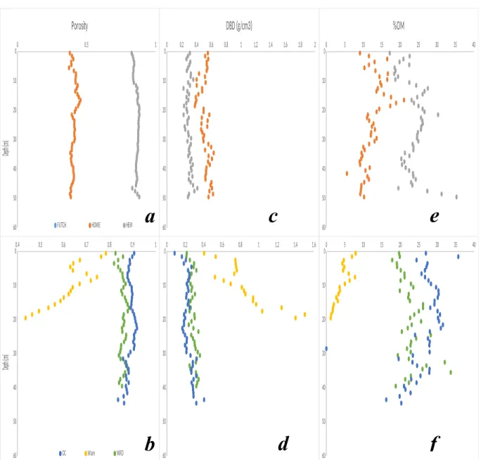
Porosity
In New Hanover County, FU showed a decrease in porosity from 0.87 to 0.61 from the
top of the core to the bottom of the core. Both HEW and HOW displayed little variation in their
porosity throughout the profile, but the average porosities of 0.86 and 0.41, respectively, differed
greatly (Fig. 2a). There was little variation in porosity as a function of depth between WARD
and OC and the average porosity was 0.85 and 0.89 respectively. WARE, also among the
Carteret County sites, experienced a change in porosity from approximately 0.78 at the top of the
soil profile to 0.43 at the bottom (Fig. 2b).
Dry Bulk Density (DBD)
Dry bulk density (g cm-3) was constant between both HOWE and HEW with average
values of 0.51 g/cm3 and 0.29 g/cm3. DBD increased with depth at FU from 0.26 g/cm3 to 0.9
g/cm3 from the top to the bottom of the core (Fig. 2c). The two cores that did show a positive
relationship relationship exhibited a positive relationship and were the two shortest cores taken
(FU and WARE). FU showed an increase range from 0.3 to 1.0 g/cm3 and WARE exhibited an
increase from roughly 0.5 to 1.5 g/cm3 (Fig. 2d). In Carteret County, both WRD and OC were
similarly stable with little variation throughout the core in regards to DBD.
Percent Organic Matter (%OM)
Organic matter composition correlated negatively with depth across FU. FU decreased
from 16.8 percent to 3.30 percent while HOW showed no significant change as a function of
depth and HEW increased from17.2 to 35.3 percent (Fig. 2e). A Positive correlations was also
found at both WARD, which increased from 19.7 percent to 22.4 percent. Both OC and WARE
the lowest %OM among the site in Carteret County, to 1.18 percent. The decrease at OC was of a
lesser magnitude from 27.0 percent at the surface to 20.3 percent at the bottom of the core (Fig.
2f).
0 0.5 1
0 10 20 30 40 50 60 Porosity
FUTCH HOWE HEW
Dep
th (
cm)
0 0.2 0.4 0.6 0.8 1 1.2 1.4 1.6 1.8 2 0 10 20 30 40 50 60 DBD (g/cm3)
0 5 10 15 20 25 30 35 40 0 10 20 30 40 50 60 %OM
0.4 0.5 0.6 0.7 0.8 0.9 1 0 10 20 30 40 50
60 OC Ware WRD
Dep
th (
cm)
0 0.2 0.4 0.6 0.8 1 1.2 1.4 1.6 0 10 20 30 40 50 60
0 5 10 15 20 25 30 35 40 0 10 20 30 40 50 60
Figure 2 – Porosity (a,b), DBD (c,d), and %OM (e,f) as a function of depth to scale between
sites and cores. Wilmington measurements are on the top row while New Hanover measurements are on the bottom. Both WARE and FU exhibited decreases in porosity as a function of depth while all other cores remained relatively constant. WARE and FU creek experienced the greatest increase in DBD as a function of depth. %OM varied widely between cores within and across sites. WARD and HEW exhibited increases in %OM with depth. Values that appear on the y-axis are a result of missing data in regards to one of the elements.
a
c
e
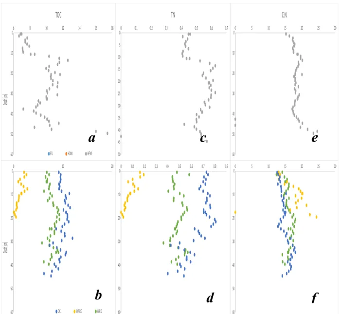
Total Organic Carbon (TOC)
At shallow depths, FU, HEW, and HOW have relatively similar carbon content (an
average of 4.69, 7.16 ,2.99 percent carbon across the first five centimeters respectively). FU
experiences an inverse relationship with depth as the carbon content decreases to 0.53 percent
25cm deep. HEW’s carbon content correlates positively with depth as the deepest subsample has
a carbon content of 17.40 percent and the last four centimeters of the core experiences an
increase of 8 percent. In HOW, carbon content increased in the first 15 centimeters from
approximately 2.99 percent to 8.21 percent from before decreasing to an average of 4.77 percent
for the remainder of the core (Fig. 3a).The organic carbon profile of both OC and WARD had
little variation as a function of depth with average percentages of 9.78 and 7.70. WARE had an
average of 1.24 percent organic carbon and also had a larger difference in surface and deep
carbon content (Fig. 3b).
Total Nitrogen (TN)
The initial composition of TN in the surface sediment between FU, HEW, and HOW
ranged from 0.20 to 0.44 percent. HOW showed a slight spike in nitrogen content at about 16
centimeters deep, which was mirrored in HEW at 13 centimeters. After this increase, the
nitrogen content drops down to an average of 0.27 percent for the remaining 34 centimeters in
HOW. HEW increases from 0.44 percent at the surface to 0.74 percent 50 centimeters deep. The
largest increase occurred during the last four centimeters when the concentration increased from
0.43 percent to 0.74 percent. FU experienced a decline in nitrogen concentration from 0.36
percent at the surface to .02 percent at the bottom of the core, 25 centimeters deep (Fig. 3c). At
Carteret County, the range of initial concentrations of nitrogen varied greater with WARE
remains relatively stable for both OC and WARD with WARD experiencing a slight decrease in
concentration after 35 centimeters. WARE exhibits the most amount of change as the
concentration changes from 0.16 to 0.02 percent from the top of the core to the bottom 20
centimeters deep (Fig. 3d).
C:N Ratios
Carbon to nitrogen ratios indicate the relative magnitude of elemental concentration in
relation to the other element. In this depiction, if the number is greater than one, carbon is
relatively greater than the nitrogen within the same sample. If the number is less than one,
nitrogen is relatively greater. Expectedly, the concentration of nitrogen was never higher than the
concentration of carbon. Linear regressions suggest that there is a close positive relationship
between TN and TOC across all sites (Fig. 3e, 3f). The two shortest cores, FU and WARE,
experienced slight increases in the C to N ratio from the top to the bottom of the core while the
6 8 10 12 14 16 18 0 10 20 30 40 50 60 TOC
FU HOW HEW
Dep
th (
cm)
0 0.1 0.2 0.3 0.4 0.5 0.6 0.7 0 5 10 15 20 25 30 35 40 45 50 TN
0 5 10 15 20 25 30 0 10 20 30 40 50 60 C:N
0 10 20
0 10 20 30 40 50
60 OC WARE WRD
Dep
th (
cm)
0 0.1 0.2 0.3 0.4 0.5 0.6 0.7 0.8 0.9 0 10 20 30 40 50 60
0 5 10 15 20 25 30 0 10 20 30 40 50 60
Figure 3 – Total Organic Carbon (a,b), Total Nitrogen (c,d), and the ratio of TOC to TN (e,f) as
a function of depth to scale between sites and cores. New Hanover County sites’ measurements are on the top row while Carteret County sites’ measurements are on the bottom. TOC remained relatively constant across the cores as a function of depth, except for WARE and FU which both exhibited decreased concentrations at the bottom. Relatively stable levels of N composition were present across all cores except for a similar decrease among WARE and FU once again. WARE experienced the greatest increase in C:N over depth, but for the most part, all the sites had stable values as a function of depth. Values that appear on the y-axis are a result of missing data in regards to one of the elements.
Radioactive Geochronometer Depth Profiles and Accumulation Rates
Sediment accumulation rates (SAR) and sediment dating was predicted using the
Activity (Constant Initial Concentration), Constant Sedimentation models, and 137Cs as an
independent chronometer (Appendix Fig. 16, Fig. 17). Excess 210Pb is the amount of 210Pb isotope
in excess to background 210Pb produced by 226Ra decay in sediments. Background levels of 210Pb
are reach when the total 210Pb is approximately equal to 226Ra, which means that excess 210Pb is
zero. Throughout the entirety of the core from WARD, the background level was never reached
(Appendix Fig. 16). The three models outlined in Sanchez-Cabeza and Ruiz-Fernàndez (2012)
depend on reaching background levels of 210Pb for accurate approximations. When background
levels are not reached, the excess 210Pb activity when the change in excess 210Pb activity is zero is
used as a proxy for background radiation. WARE experienced base levels of excess 210Pb
approximately 20 cm deep (Appendix Fig. 16). At OC, the background levels were estimated at
approximately 30 cm deep (Appendix Fig. 16). At the sites within New Hanover County,
background was reached at depths of approximately 14 cm for HOW (Appendix Fig. 17).
Background was not reached at either HEW or FU so the activity at 24 and 25 cm deep was used
as a proxy (Appendix Fig. 17).
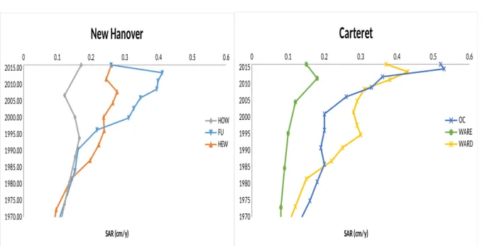
SAR increased from 1970 to 2016 across all sites within Carteret County. WARE
experienced the smallest increase in SAR, 0.07 cm/y, while OC increased by 0.46 cm/y and
WARD increased by 0.32 cm/y. All sites in the region showed a sharp decline in their last
interval. WARE decreased from 0.18 cm/y to 0.15 cm/y, WARD decreased from 0.43 cm/y to
0.37 cm/y, and OC decreased from 0.53 cm/y to 0.52 cm/y. SAR correlated positively across
time for all sites within New Hanover County as well. FU experienced positive changes in SAR
over time across all intervals, except for a sharp decline from 0.41 cm/y to 0.26 cm/y between
and 2011 while HOW also experienced a slight decline, from 0.17 to 0.12 from 1993 to 2006
(Fig. 4).
0 0.1 0.2 0.3 0.4 0.5 0.6
1970.00 1975.00 1980.00 1985.00 1990.00 1995.00 2000.00 2005.00 2010.00 2015.00
New Hanover
HOW FU HEW SAR (cm/y)0 0.1 0.2 0.3 0.4 0.5 0.6
1970 1975 1980 1985 1990 1995 2000 2005 2010 2015
Carteret
OC WARE WARD SAR (cm/y)Figure 4 – SAR (cm/y) derived from using the Constant Flux (Constant Rate of Supply) model
outlined in Sanchez-Cabeza and Ruiz-Fernandéz (2012). SAR at the surface segments (dated 2016) have low confidence given the sources of error that may have resulted from the sampling technique. The y-axis is the year that the sediment was deposited.
Land Cover Projection
Watersheds for each tidal creek were approximated using topography from NConemap.
In Carteret County, this resulted in watersheds of areas 2.57, 54.0, and 23.7 km2 for WARE,
WARD, and OC respectively. Due to the overall low elevation throughout the county, and
especially in the approximated watersheds of OC and WARE, boundaries of the watershed are
approximate and these projected watersheds may have a greater extent than other models
(Appendix Fig. 18). In comparison to watersheds derived from USGS StreamStats, the
watersheds approximated in this study were larger by 8 to 25 percent. In New Hanover County,
the changes in elevation in the study sites were greater, which allowed for better defined
9.65 km2 respectively and exceeded the watersheds predicted by USGS StreamStats by 5 to 10
percent.
The classified maps projected for both counties utilized training data specific to the
individual regions and consisted of five classes: Water, Wetland, Vegetated Undeveloped (ex.
shrublands), Agricultural, and Urban. Accuracy was determined using a contingency table as
well as the Kappa statistics, a measure of the overall accuracy that was corrected for the
probability that a pixel was correctly classified due to random chance. The map of Carteret
County had a final overall accuracy of 63.5% (Fig. 5) while the New Hanover classification was
54.8% accurate (Fig. 6). When the Urban class is removed from the accuracy assessment, the
accuracies for Carteret and New Hanover county increase by approximately 3 and 11 percent.
This is likely due to the misclassification of sand as urbanized areas given their relatively similar
reflectance values. Therefore, in approximating the total amount of area of each class, pixels
classified as Urban have errors of 2, 4, and 3 percent in the WARE, WARD, and OC watersheds
and errors of 6, 10, and 14 percent for the HOW, HEW, and FU watersheds. The higher errors
among the sites in New Hanover county are most likely due to increased concentrations of sand
as a result of shallower creek beds and smaller shore to barrier island distances in the intercostal
Figure 5 – A projection of Carteret county with inlaid maps of the study sites WARE, WARD, and OC from West to East. Blue pixels represent water. Orange pixels represent agricultural land. Black pixels represent urban lands, roads, and areas with large amounts of sand. Yellow pixels represent undeveloped lands, such as shrublands, grass fields, and forests. Finally, green areas represent wetlands. This image was taken on June 9th, 2016 by Landsat 8 and is available
Figure 6 - A projection of New Hanover county with inlaid maps of the study sites HEW, HOW, and FU from South to North. Blue pixels represent water. Orange pixels represent agricultural land. Black pixels represent urban lands, roads, and areas with large amounts of sand. Yellow pixels represent undeveloped lands, such as shrublands, grass fields, and forests. Finally, green areas represent wetlands. This image was taken on May 15th, 2016 by Landsat 8 and is available
Discussion:
Sediment Classification
Percent organic matter (%OM) can be used in conjunction with other morphological
characteristics as a rough delineation between marsh and marine sediment. Typically, a greater
%OM is indicative of marsh sediment while lower values are considered marine sediment
(Burdige 2007). According to this guideline, the WARE site likely exhibited marine sediments
throughout its depth profile while most of the other sites, except for FU deeper than 21 cm and
HOWE deeper than 40 cm, likely exhibited marsh sediment throughout their profiles (Fig. 2e, 2f,
7).
Studies have also used DBD as an indication of marine sediment, where estimates of
marine sediment DBD should be in the range of 1.70 to 1.95 g/cm3 (Sykes 1996). Given the high
porosity and large amount of water found in most marsh sediments, it is expected that marsh
sediments have lower DBDs in comparison to marine sediments (Bradley and Morris 1990).
Both the WARE and FU sites experienced a rapid increase in DBD at the bottom of the sampled
core, but both sites had values (1.50 g/cm3 and 0.90 g/cm3 respectfully) that were below the range
outlined in Sykes (1996). Throughout all samples, according to the DBD definition of marine
sediment, marine sediment was absent (Fig. 2c, 2d).
Atomic C:N ratios can be used to distinguish between algal and terrestrial plant origins of
organic matter in the sediment (Meyers and Shaw, 1996). Typically, algae have a C:N ratio in
the range of 4 to 10 while vascular plants have a C:N ratio of 20 or greater (Premuzic et al. 1982;
Jasper and Gagosian 1990; Meyers 1994; Prahl et al. 1994). Since salt marshes often experience
fluxes of organic matter from both terrestrial and aquatic reservoirs, C:N values in the range of
ratios range from 10 to 20 showing marsh derived organic matter, except for in the deepest
sections of WARE, which has a C:N greater than 20 and is indicative of the burial of vascular
plants at that depth. The majority of the sites in New Hanover county also range from 10 to 20
except for the last five centimeters of HEW, the last sample from FU, and one sample close to
the surface of HOW. Therefore, at both sites, a majority of the sediment sampled had C:N
indicative of marsh sediments (Fig. 3e, 3f).
These three methodologies (%OM, DBD, and C:N) all indicate that a majority of the
sediment sampled can be considered marsh sediments. The most striking difference between the
classifications of three methodologies is in regards to WARE, which was classified as entirely
marine sediment by the %OM approximation, while none of the sediments in the core were
classified as marine by the DBD method and only the deepest samples were considered marine
by the C:N method. Given the lower porosity and higher DBD found at WARE, the content of
smaller sized particles at WARE may be higher than the other sites, which could partially explain
the difference between methods. One possible reason that a majority of the sites did not exhibit
marine sediment throughout their core could be the sampling method. Since aluminum push
cores are driven into the ground by the sampler, the sampling limit is dependent on the strength
of the sampler. Therefore, marine sediments, which are denser and harder to core through, often
Figure 7 – The percent organic material, inorganic carbon, and mineral content of the cores at 1 cm interval. The x-axis represents percentage on a log scale while the y-axis serves as an
indicator of depth (cm).
Carbon Models
North Carolina boasts a considerable history of research regarding changes in sediment
accretion and carbon burial across the marine landscape. For example, organic carbon
concentration and burial fluxes have been studied on the continental slope off the shore of Cape
Hatteras (Alperin et al. 2002; Thomas et al. 2002; Alperin et al. 1999). Closer to the shore of
North Carolina, not only has the blue carbon content of barrier islands been explored, but the
manner in which global changes affect the carbon capacity of these systems as well (Theuerkauf
and Rodriguez 2017). Among salt marshes, carbon fluxes into and out of the salt marsh and
estuarine systems from processes such as erosion and sediment accretion have been extensively
carbon signatures, morphology, and radiochemical tracers in a well studied salt marsh dominated
coastal region of North Carolina.
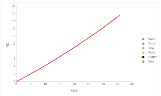
One of the seminal studies on salt marsh storage in North Carolina is by Craft et al.
(1991). In this research, they used an empirical relationship to quantify the correlation between C
concentration and %OM. This relationship was significant due to the ease and inexpensive nature
of measuring %OM in comparison to directly measuring C concentration, which requires
specialized instrumentation and can often be costly. Although %OM cannot be used directly
determine carbon burial rates, %OM is an indirect measure of C. Therefore, the ability to convert
%OM values to C values allows for cheaper and quicker estimations of C storage. Craft et al.
(1991) discovered an expeditious process to quantify C storage and made it more accessible for
scientists globally to conduct similar research.
It is important to note that Craft et al. (1991) presented an equation used to estimate %C
from %OM that was constructed from measurements in coastal North Carolina. As this equation
became increasingly well-received, it has been applied to many other locations to represent the
relationship between %OM and C composition of salt marshes far outside of the original study
area from Tampa Bay, to San Francisco Bay, and to Noord Friesland Buitendijks, Netherlands
(Radabaugh et al. 2017; Murphy et al. 2017; Müller 2017). The function of the relationship is
unquestionable since %OM is C based, but an empirical relationship that was developed for a
single salt marsh on the mid-Atlantic coastline of the US may not be representative of all
marshes around the world, especially considering advances in modern salt marsh research.
Recent studies have shown that sedimentation rates and sediment provenance, two factors that
influence C content of marshes, vary globally. Primary productivity, in addition to plant
greatly impact the relationship between C and %OM, thus the empirical relationship between the
measures are impacted.
This study compares %OM from loss on ignition and %TOC derived from elemental
combustion to the values that would be predicted by Craft et al. (1991) to understand the
continued application of the relationship in NC (Fig. 8). These data shows that the Craft
relationship would have over-predicted %TOC values based on %OM. It should be noted that
while both the data from this study and Craft et al. (1991) originated from geographically close
study areas, this fact does not invalidate the applicability of the model. Scientists have since
determined that small variations in geomorphology and vegetation composition can have
significant effects in altering both %OM and %TOC. These data illustrates this fact and suggest
that the empirical relationship from Craft et al. (1991) should be updated using more recent data.
Additional modifications to the original Craft et al. (1991) model may also be needed depending
on specific study site conditions such as decomposition rate or organic matter sources may be
necessary to produce accurate data.
The comparison done in this study not only serves the purpose of validating the observed
relationship between %OM and C, but it also emphasizes the importance of updating
relationships as the conditions surrounding marsh ecosystems change. Likewise, these data
illustrate the need to develop empirical relationships for different areas of the world to account
for unique sediment, productivity, and climate variations. Craft et al. (1991) created an empirical
formula that was based on a specific region, brackish salt marshes in North Carolina, which were
not distant from sites where this study was conducted. Given the differences in trends between
the two relationships, this indicates that more recent developments, such as increasing urbanized
0 5 10 15 20 25 30 35 40 0
2 4 6 8 10 12 14 16 18 20
Ware Futch Hew Ward Oyster How
%OM
%
C
Figure 8 – The observed relationship between percent organic material and percent carbon in
comparison to the predicted relationship (dark red) described by Craft et al. 1991
SAR and rSLR
Marsh accretion rates (MAR) and carbon accretion rates (CAR) are inherently correlated
with SAR seeing as MAR is the product of DBD and SAR and CAR is the product of MAR and
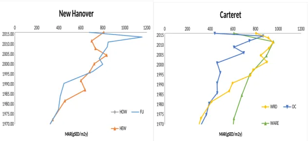
C content. Within Carteret County, there was an overall positive trend in MAR between all the
sites. In the youngest, and shallowest, segment of all the cores there was a sharp decline in MAR,
especially at OC and WARE (Fig. 9). While decreases in SAR were seen during the same period,
the magnitude of the decreases are far greater. This typically means that the DBD experienced a
decrease over that period. Although these sites did exhibit decreases in DBD, likely due to plant
roots, in this section of the cores (Fig. 2f), this sharp decline is likely the result of sampling error.
As samples are taken, the surface sediment is likely disturbed. While this study did have a 1 cm
interface layer to account for this, there still may have been disturbances found within the surface
methodological error. MAR and SAR are relatively similar in shape for New Hanover county,
which is due to the relatively constant DBD in the shallow depths of the core (Fig. 2e).
0 200 400 600 800 1000 1200
1970.00 1975.00 1980.00 1985.00 1990.00 1995.00 2000.00 2005.00 2010.00 2015.00
New Hanover
HOW FU
HEW
MAR(gSED/m2y)
0 200 400 600 800 1000 1200
1970 1975 1980 1985 1990 1995 2000 2005 2010 2015
Carteret
WRD OC
WARE
MAR(gSED/m2y)
Figure 9 - MAR (gSED/m2y) derived by finding the product of the DBD and SAR at specific
depths. Similar to SAR, the surface segments (dated 2016) have low confidence given the sources of error that may have resulted from the sampling technique. The y-axis is the year that the sediment was deposited.
Carbon burial (CAR) is the fraction of the total accumulation of mass that is carbon. In
Carteret County, it can be seen that overall the carbon content of WARE was much less than that
of WARD or OC. OC in comparison to WARD has a slightly higher C content (Fig. 10). In New
Hanover County, the carbon content of HEW was the highest throughout the profile. Both FU
0 20 40 60 80 1970.00 1975.00 1980.00 1985.00 1990.00 1995.00 2000.00 2005.00 2010.00 2015.00
New Hanover
HOW FU HEW CAR(gC/m2y)0 10 20 30 40 50 60 70 80 90
1970 1975 1980 1985 1990 1995 2000 2005 2010 2015
Carteret
WRD OC WARE CAR(gC/m2y)Figure 10 – CAR (gC/m2y) derived by finding the product of the proportion of carbon by weight
and MAR at specific depths. Similar to SAR and MAR, the surface segments (dated 2016) have low confidence given the sources of error that may have resulted from the sampling technique. The y-axis is the year that the sediment was deposited.
CAR is the product of MAR and the C concentration at the sample level therefore
graphing CAR as a function of MAR will be able to quantify the variation of C concentration
within and between cores (Fig. 11). Within site variation is expressed through the R-squared
values. If C concentration is relatively constant in a single core (site), it is expected that the
relationship between MAR and CAR will be strongly linear. A strong linear relationship can be
found at OC, WARD, FU, and HEW, which all have R-squared values greater than or equal to
0.933. WARE and HOWE exhibit R-squared values of 0.493 and 0.007, respectfully, which
indicates a greater amount of variability between sampled segments in the core. This lack of
covariance is confirmed by Fig. 3a and Fig. 3b where concentration varied in the shallowest
sediments as a function of depth in both cores. Considering that the slope of Fig. 11 represents
the change in CAR over the change in MAR, this relationship can be reduced to the average
the slope, and variation within a core, the R-squared (Table 2); samples with high concentrations
of C (OC, HEW, WARD) also had less variation in the measured sediments while sediments
with the low C concentration (HOW, WARE, FU) had higher amounts of variation in the
sampled sediments. The results indicate that the higher the average C concentration, the less
variability within a core one should see as a function of depth at shallow depths. This could be
Table 2 – The slopes and R2 values of the linear relationships exhibited between MAR and CAR
in Fig. 11. with site, site ID, and region.
REGION SITE SITE ID SLOPE R-SQUARED
CARTERET
COUNTY Oyster Creek OC 0.0907 .985
Ward Creek
WARD 0.0673 .979
Ware
Creek WARE 0.0242 .493
NEW HANOVER COUNTY
Futch
Creek FU 0.0431 .933 Hewletts
Creek HEW 0.0627 .956 Howe
0 200 400 600 800 1000 1200 1400 0
10 20 30 40 50 60 70 80 90
FU Linear (FU) HEW Linear (HEW) HOW Linear (HOW) OC
Linear (OC) WARE Linear (WARE) WRD
Linear (WRD)
MAR
C
A
R
Figure 11 – The relationship between MAR and CAR at similar sample depths. Only samples
dating back to approximately 1970 were considered excluding the surface sample, which expressed a highly variable SAR possibly due to the sampling method.
indicative of lower confidence in the sampling method used to measure C at low concentrations.
It should also be noted that when considering all samples between cores, the relationship was
weaker than a majority of those seen within cores (R2=.276).
From approximately 2005 to 2010 among all sites within Carteret County, increasing
rates of sediment accretion were observed. Sea level during this period was also rising more
rapidly compared to the previous ten years of data (Fig. 12). Sea level continued to rise after
2010, but this effect was not reflected by a similar increase in the sediment accumulation rates
(SAR) (Fig. 12). Instead, SAR exhibited a 1.9% decrease at OC, a 13.9% decrease at WARD,
and a 16.7% decrease at WARE. A reduction in sediment loading correlates with the
construction of reservoirs and dams, which have the ability to trap approximately 50% of
regional sediment flux (Syvitski et al. 2005). Specifically, the Gallants Channel Bridge began
determinant for the observed decrease in sediment accretion, but bridges have been shown to
baffle water currents, which reduces sediment load capacity (Furniss et al. 1991). Another factor
that may have influenced SAR was the conversion of 0.94 miles of agricultural and 0.44 square
miles of grasslands to developed land (https://coast.noaa.gov/ccapatlas/).
The NOAA tides and currents monitoring station in Wilmington, North Carolina showed
a positive trend in rSLR from 1970 to the end of the monitoring period in 2016, which was
mirrored in the change of SAR between all the sites within New Hanover County (Fig. 13). This
correlation is congruent with the general relationship between SLR and SAR, due to the effects
of SLR on inundation time, the period in which sediment is deposited in tidal marshes. The
NOAA station also measured accelerated rates of rSLR starting in 2010 and continuing until the
end of the monitoring period in 2016. The only site within New Hanover county that had a
similar positive trend in its SAR over the period was HOW. FU increased slightly from 2010 to
2013, but showed a sharp decrease from 0.41 cm/y to 0.26 cm/y between 2013 and 2016 and
resulted in an overall negative trend from 2010 to 2016 and HEW decreased slightly over the
1970 1975 1980 1985 1990 1995 2000 2005 2010 2015 20200 2 4 6 8 10 12 -0.3 -0.2 -0.1 0 0.1 0.2 0.3
Carteret
OC WARE WARD Car. SLR S A R ( c m / y ) S e a L e v e l (m )Figure 12 – Sediment accretion rates (cm/y) derived from 210Pb analysis compared to height of
the sea level above the sea level in 1901 measured at the NOAA station in Beaufort, North Carolina. The solid black line represents the average sea level rise over a roughly thirty-year period.
Reasons for a decrease in SAR in New Hanover in the face of increased rSLR can be
resultant for many of the same, general reasons a decrease in SAR was seen in Carteret County.
Specific incidences that may have contributed to this trend may have been an increase in high
intensity developed space and grasslands, which reduce the sediment loading contributed by
barren lands. Throughout the county, the amount of developed area increased by 14.08% and the
amount of impervious surfaces increased by 17.01% from 1996 to 2010 (CCAP). The amount of
barren area, which typically increases the amount of sediment loading to watershed, increased by
0.80 square miles during the same time period and the expected increased trend in SAR is shown
between all sites within the county. It should be noted that these trends are for the entire county
197 0.0
0 198
0.0 0 199
0.0 0
200 0.0
0 201
0.0 0 202
0.0 0 -0.1 -8.32667268468867E-17 0.1 0.2 0.3 0.4 0.5 0.6 -0.3 -0.2 -0.1 -5.55111512312578E-17 0.1 0.2 0.3
New Hanover
HOW FU HEW NH. SLR S A R ( c m / y ) S e a L e v e l (m )Figure 13 – Sediment accretion rates (cm/y) derived from 210Pb analysis compared to height of
the sea level above the sea level in 1901 measured at the NOAA station in Wilmington, North Carolina. The solid black line represents the average sea level rise over a roughly thirty-year period.
SAR and Land Cover
Two ways that marshes persist in the face of rising sea levels is by either vertical
accretion or horizontal migration. SAR is a relative representative of vertical accretion seeing as
most of the matter that gathers on the surface of marshes is predominantly mineral (Fig. 3).
Therefore, a relationship between land cover and SAR is expected, but this is not seen in the
provided data (Fig. 14). Horizontal migration is not a direct function of land cover, but still relies
on adjacent land matrices to occur. The process of horizontal migration typically occurs when
landward ecosystems, typically marine forests, experience die off from saltwater intrusions and
salt marsh grasses act as early successional species and begin to propagate in that area. The
amount of marine forest die-off correlates with sea level rise, so as sea level rises, it is expected
that there should be a horizontal migration of the marsh. This process is dependent on the
presence of an area for the salt marsh to migrate into. Therefore, the development and
0.1 0.15 0.2 0.25 0.3 0.35 0.4 0.45 0.5 0.55 0.6 0 10 20 30 40 50 60 70 80 90 URBAN Linear (URBAN) AGRICULTURAL Linear (AGRICULTURAL) UNDEVELOPED Linear (UNDEVELOPED) WETLAND Linear (WETLAND) SAR (cm/y) Pe rc en t o f L an d Co ve r
Figure 14 – SAR (cm/y) from all sites compared with the composition of the modern land cover
within the site. R-squared values ranged from 0.04, agricultural land, to 0.27, wetlands. SAR come from not the surface sample, but from the sample immediately beneath it so as to compensate for any disturbances in the soil caused by the sampling method.
Sediment accumulation rates do not appear to vary with modern land cover composition
(Fig. 14). In areas where agricultural land dominated, WARD and HEW, sediment accumulation
rates varied by nearly .2 cm/y and the two areas with the smallest amount of agricultural land,
differed by .3 cm/y. Urban and undeveloped land had similar scattered trends while wetland
extent seemed to be the most predictive of high sediment accretion rates. A more useful way to
view this data may be to compare the amount of developed, urban and agricultural, land to the
amount of natural, wetlands and undeveloped regions, landscape. When viewed this way, it can
be seen that OC and WARE were the only watersheds to be dominated by undeveloped land
(Fig. 15). While WARE does boast the lowest SAR for either region, OC actually boasts the
highest rates of modern accretion. These trends further support the idea that SAR vary
independently of land cover. Given that there are only six data points within each category, it
OC
WRD
WARE
FU
HOW
HEW
0% 10% 20% 30% 40% 50% 60% 70% 80% 90% 100%
Landcover Composition in Site Watersheds
URBAN AGRICULTURAL UNDEVELOPED WETLAND
Figure 15 – The breakdown of land cover composition into the classified categories defined by
training data specific to each region. WARD was the only watershed from Carteret County to be comprised of predominantly developed land, agricultural and urban lands, while all the
watersheds within New Hanover were dominated by developed landscapes.
Summary:
From the data involved and collected during this study, three major conclusions can be
made regarding the Craft model for C concentration prediction, sediment accretion rates, rSLR,
and land cover:
1. The empirical relationship relating %OM to carbon concentration proposed in Craft et al.
(1991) was specific to a study site, but when sites in the same relative geographical area
were sampled nearly 25 years later, the Craft model over predicted carbon concentrations
consistently, which highlights the necessity to both update the model to include modern
global changes, especially sea level rise, and to adapt the model to fit the researcher’s
specific study area.
3. Although land use does not seem to correlate with changes in the accumulation of
modern sediments, increased urbanization along lands adjacent to wetlands may inhibit
marshes ability to migrate laterally, a survival mechanism in the face of accelerated sea
level rise.
Additional information regarding historical changes in land cover could help inform the effects,
or lack thereof, of changes in land cover composition on SAR in tidal creek marshes. While this
study does parse the different components of accreted sediment into organic, inorganic, and
mineral categories, it does not consider the source of these proponents. Additional data from
methodologies, such as mass spectroscopy and grain size analysis, could help inform the
importance of land use change by emphasizing where sources were originating from. Linking
SAR and changes in land cover has the potential to inform management of effects that
downstream wetlands could experience due to upstream changes in regards to both the longevity
References:
Alperin, M. J., Martens, C. S., Albert, D. B., Suayah, I. B., Benninger, L. K., Blair, N. E., & Jahnke, R. A. (1999). Benthic fluxes and porewater concentration profiles of dissolved organic carbon in sediments from the North Carolina continental slope. Geochimica et
Cosmochimica Acta, 63(3-4), 427-448.
Alperin, M. J., Suayah, I. B., Benninger, L. K., & Martens, C. S. (2002). Modern organic carbon burial fluxes, recent sedimentation rates, and particle mixing rates from the upper
continental slope near Cape Hatteras, North Carolina (USA). Deep Sea Research Part II:
Topical Studies in Oceanography, 49(20), 4645-4665.
Appleby, P. G. (2002). Chronostratigraphic techniques in recent sediments. In Tracking
environmental change using lake sediments (pp. 171-203). Springer, Dordrecht.
Armentano, T. A., & Woodwell, G. M. (1975). Sedimentation rates in a Long Island marsh determined by 210Pb dating. Limnology and Oceanography, 20(3), 452-456.
Bradley, P. M., & Morris, J. T. (1990). Physical characteristics of salt marsh sediments: ecological implications. Marine Ecology Progress Series, 245-252.
Burdige, D. J. (2007). Preservation of organic matter in marine sediments: controls, mechanisms, and an imbalance in sediment organic carbon budgets?. Chemical reviews, 107(2), 467-485.
Callaway, J. C., Borgnis, E. L., Turner, R. E., & Milan, C. S. (2012). Carbon sequestration and sediment accretion in San Francisco Bay tidal wetlands. Estuaries and Coasts, 35(5), 1163-1181.
Colman, S. M., & Bratton, J. F. (2003). Anthropogenically induced changes in sediment and biogenic silica fluxes in Chesapeake Bay. Geology, 31(1), 71-74.
Couto, T., Duarte, B., Caçador, I., Baeta, A., & Marques, J. C. (2013). Salt marsh plants carbon storage in a temperate Atlantic estuary illustrated by a stable isotopic analysis based approach. Ecological indicators, 32, 305-311.
Craft, C. B., Broome, S. W., Seneca, E. D., & Showers, W. J. (1988). Estimating sources of soil organic matter in natural and transplanted estuarine marshes using stable isotopes of carbon and nitrogen. Estuarine, Coastal and Shelf Science, 26(6), 633-641.
Dahdouh-Guebas, F., Jayatissa, L. P., Di Nitto, D., Bosire, J. O., Seen, D. L., & Koedam, N. (2005). How effective were mangroves as a defence against the recent tsunami?. Current
biology, 15(12), R443-R447.
Dingman, S. L. (2002). Water in soils: infiltration and redistribution. Physical hydrology.
Friedl, M. A., Sulla-Menashe, D., Tan, B., Schneider, A., Ramankutty, N., Sibley, A., & Huang, X. (2010). MODIS Collection 5 global land cover: Algorithm refinements and
characterization of new datasets. Remote sensing of Environment, 114(1), 168-182.
Furniss, M. J., Roelofs, T. D., & Yee, C. S. (1991). Road construction and
maintenance. American Fisheries Society Special Publication, 19, 297-323.
Gupta, S., & Larson, W. E. (1979). Estimating soil water retention characteristics from particle size distribution, organic matter percent, and bulk density. Water resources
research, 15(6), 1633-1635.
Håkanson, L. & Jansson, M. (1983). Physical and Chemical Sediment Parameters. In Principles
of lake sedimentology, pp. 73-113. Berlin: Springer-Verlag.
Hinrichsen, D. (1999). Coastal waters of the world: trends, threats, and strategies. Island Press.
Holmén, K. (2000). The global carbon cycle. In International Geophysics (Vol. 72, pp. 282-321). Academic Press.
Howard, J., Sutton-Grier, A., Herr, D., Kleypas, J., Landis, E., Mcleod, E., ... & Simpson, S. (2017). Clarifying the role of coastal and marine systems in climate mitigation. Frontiers
in Ecology and the Environment, 15(1), 42-50.
Jasper, J. P., & Gagosian, R. B. (1990). The sources and deposition of organic matter in the Late Quaternary Pigmy Basin, Gulf of Mexico. Geochimica et Cosmochimica Acta, 54(4), 1117-1132.
Kemp, A. C., Vane, C. H., Horton, B. P., & Culver, S. J. (2010). Stable carbon isotopes as potential sea-level indicators in salt marshes, North Carolina, USA. The Holocene, 20(4), 623-636.
Kirwan, M. L., & Megonigal, J. P. (2013). Tidal wetland stability in the face of human impacts and sea-level rise. Nature, 504(7478), 53.
Kirwan, M. L., Murray, A. B., Donnelly, J. P., & Corbett, D. R. (2011). Rapid wetland expansion during European settlement and its implication for marsh survival under modern
sediment delivery rates. Geology, 39(5), 507-510.
Lei, C., Jin-ming, S. O. N. G., Xue-gang, L. I., Hua-mao, Y. U. A. N., Ning, L. I., & Li-qin, D. U. A. N. (2013). Deposition and burial of organic carbon in coastal salt marsh: Research progress. Yingyong Shengtai Xuebao, 24(7).
Leonard, L. A., & Croft, A. L. (2006). The effect of standing biomass on flow velocity and turbulence in Spartina alterniflora canopies. Estuarine, Coastal and Shelf Science, 69 (3-4), 325-336.
Loomis, M. J., & Craft, C. B. (2010). Carbon sequestration and nutrient (nitrogen, phosphorus) accumulation in river-dominated tidal marshes, Georgia, USA. Soil Science Society of
America Journal, 74(3), 1028-1036.
Mcleod, E., Chmura, G. L., Bouillon, S., Salm, R., Björk, M., Duarte, C. M., ... & Silliman, B. R. (2011). A blueprint for blue carbon: toward an improved understanding of the role of vegetated coastal habitats in sequestering CO2. Frontiers in Ecology and the
Environment, 9(10), 552-560.
Meyers, P. A. (1994). Preservation of elemental and isotopic source identification of sedimentary organic matter. Chemical geology, 114(3-4), 289-302.
Meyers, P. A., & Shaw, T. J. (1996). Organic Matter Accumulation, Sulfate Reduction, and Methanogenesis in Pliocene–Pleistocene Turbidites on the Iberia Abyssal Plain.
In Proceedings of the Ocean Drilling Program, Scientific Results (Vol. 149, p. 705).
Moore, W. S. (1984). Radium isotope measurements using germanium detectors. Nuclear
Instruments and Methods in Physics Research, 223(2-3), 407-411.
Morris, J. T., Sundareshwar, P. V., Nietch, C. T., Kjerfve, B., & Cahoon, D. R. (2002). Responses of coastal wetlands to rising sea level. Ecology, 83(10), 2869-2877.
Ninan, K. N. (Ed.). (2014). Valuing ecosystem services: methodological issues and case studies. Edward Elgar Publishing.
Pendleton, L., Donato, D. C., Murray, B. C., Crooks, S., Jenkins, W. A., Sifleet, S., ... & Megonigal, P. (2012). Estimating global “blue carbon” emissions from conversion and degradation of vegetated coastal ecosystems. PloS one, 7(9), e43542.
Prahl, F. G., Ertel, J. R., Goni, M. A., Sparrow, M. A., & Eversmeyer, B. (1994). Terrestrial organic carbon contributions to sediments on the Washington margin. Geochimica et
Cosmochimica Acta, 58(14), 3035-3048.
Premuzic, E. T., Benkovitz, C. M., Gaffney, J. S., & Walsh, J. J. (1982). The nature and
distribution of organic matter in the surface sediments of world oceans and seas. Organic
Redfield, A. C. (1965). Ontogeny of a salt marsh estuary. Science, 147(3653), 50-55.
Sanchez-Cabeza, J. A., & Ruiz-Fernández, A. C. (2012). 210Pb sediment radiochronology: an integrated formulation and classification of dating models. Geochimica et Cosmochimica Acta, 82, 183-200.
Schulz, H. D., & Zabel, M. (2006). Marine geochemistry (Vol. 2). Berlin: Springer.
Stutz, M. L., & Pilkey, O. H. (2011). Open-ocean barrier islands: global influence of climatic, oceanographic, and depositional settings. Journal of Coastal Research, 27(2), 207-222.
Sykes, T. J. (1996). A correction for sediment load upon the ocean floor: Uniform versus varying sediment density estimations—Implications for isostatic correction. Marine
Geology, 133(1-2), 35-49.
Syvitski, J. P., Vörösmarty, C. J., Kettner, A. J., & Green, P. (2005). Impact of humans on the flux of terrestrial sediment to the global coastal ocean. science, 308(5720), 376-380.
Theuerkauf, E. J., Stephens, J. D., Ridge, J. T., Fodrie, F. J., & Rodriguez, A. B. (2015). Carbon export from fringing saltmarsh shoreline erosion overwhelms carbon storage across a critical width threshold. Estuarine, Coastal and Shelf Science, 164, 367-378.
Theuerkauf, E. J., & Rodriguez, A. B. (2017). Placing Barrier‐Island transgression In a Blue‐
Carbon Context. Earth's Future.
Thomas, C. J., Blair, N. E., Alperin, M. J., DeMaster, D. J., Jahnke, R. A., Martens, C. S., & Mayer, L. (2002). Organic carbon deposition on the North Carolina continental slope off Cape Hatteras (USA). Deep Sea Research Part II: Topical Studies in
Oceanography, 49(20), 4687-4709.
Wentworth, C. K. (1922). A scale of grade and class terms for clastic sediments. The journal of
Appendix:
4 6 8 10 12 14 16 0 5 10 15 20 25 30 35
Excess 210Pb (dpm/g)
0 1 2 3 4 5 6 7 8 9 0 5 10 15 20 25 30 35 40 45
Excess 210Pb (dpm/g)
-0.5 0 0.5 1 1.5 2 2.5 3 3.5 4 4.5 0 5 10 15 20 25
Excess 210Pb (dpm/g)
0 0.1 0.2 0.3 0.4 0.5 0.6 0.7 0 5 10 15 20 25 30 35 137Cs (dpm/g)
0 0.2 0.4 0.6 0.8 1 1.2 1.4 0 5 10 15 20 25 30 35 40 45 137Cs (dpm/g)
0 0.05 0.1 0.15 0.2 0.25 0.3 0 5 10 15 20 25 137Cs (dpm/g)
Figure 16 – The decays per min per gram of sediment (dpm/g) of 210Pb and 137Cs samples as a
function of depth of sites within Carteret County. True background, where excess 210Pb is in
spectral equilibrium with 226Ra, was only reached once, at WARE, and background was
estimated for OC and WARD where there was little change in dpm/g as a function of depth. 137Cs
was used as independent chronometer and the profiles help indicate the amount of mixing possible within the profile.
-0.5 0 0.5 1 1.5 2 2.5 3 3.5 4 4.5 0 2 4 6 8 10 12 14 16
Excess 210Pb (dpm/g)
0 1 2 3 4 5 6 7 8 9 0 5 10 15 20 25
Excess 210Pb (dpm/g)
0 2 4 6 8 10 12
0 5 10 15 20 25 30
Excess 210Pb (dpm/g)
0 0.02 0.04 0.06 0.08 0.1 0.12 0.14 0.16 0 2 4 6 8 10 12 14 16 137Cs (dpm/g)
0 0.05 0.1 0.15 0.2 0.25 0.3 0 5 10 15 20 25 137Cs (dpm/g)
0 0.05 0.1 0.15 0.2 0.25 0.3 0.35 0 5 10 15 20 25 30 137Cs (dpm/g)
Figure 17 – The decays per min per gram of sediment (dpm/g) of 210Pb and 137Cs samples as a
function of depth of sites within New Hanover County. True background, where excess 210Pb is
in spectral equilibrium with 226Ra, was only reached once, at HOW, and background was
estimated for HEW and FU where there was little change in dpm/g as a function of depth. 137Cs