A collocation algorithm based on quintic B-splines for the solitary wave simulation of the GRLW equation

Sharif University of Technology

Transactions B: Mechanical Engineering http://scientiairanica.sharif.edu

Research Note

A collocation algorithm based on quintic B-splines for

the solitary wave simulation of the GRLW equation

H. Zeybek

_{and S. Battal Gazi Karakoc}

a. Department of Applied Mathematics, Faculty of Computer Science, Abdullah Gul University, 38080 Kayseri, Turkey. b. Department of Mathematics, Faculty of Science and Art, Nevsehir Hac Bektas Veli University, 50300, Nevsehir, Turkey. Received 22 January 2017; received in revised form 21 January 2018; accepted 21 July 2018

KEYWORDS GRLW equation; Finite element scheme;

Quintic B-spline; Solitons; Undular bore.

Abstract. In this article, a collocation algorithm based on quintic B-splines is proposed to nd a numerical solution to the nonlinear Generalized Regularized Long Wave (GRLW) equation. Moreover, to analyze the linear stability of the numerical scheme, the von-Neumann technique is used. The numerical approach to three test examples consisting of a single solitary wave, the collision of two solitary waves, and the growth of an undular bore is discussed. The accuracy of the method is demonstrated by calculating the error in L2 and L1 norms and the conservative quantities I1, I2 and I3. The ndings are compared with those previously reported in the literature. Finally, the motion of solitary waves is graphically plotted according to dierent parameters.

© 2019 Sharif University of Technology. All rights reserved.

1. Introduction

The nonlinear wave phenomenon has an instrumental role in predicting natural events. The long waves in water of varying depths are modeled by equations of motion. The equations introduced for small amplitude waves are of nonlinear terms. The Regularized Long Wave (RLW) equation was initially introduced as a model for small-amplitude long waves on the surface of water in a channel by Peregrine [1,2]. Here, Peregrine examined the growth of an undular bore from a long wave. According to him, when the long wave of elevation travels in shallow water, it steepens and forms a bore. The RLW equation was discussed as an improved model of more common Korteweg-de Vries (KdV) equation by Benjamin et al. [3]. The KdV equation denes long waves by assuming a small

*. Corresponding author.

E-mail addresses: [email protected] (H. Zeybek); [email protected] (S. Battal Gazi Karakoc) doi: 10.24200/sci.2018.20781

wave amplitude and a large wave length in nonlinear dispersive and many other physical systems. Then, the idea of Equal Width (EW) wave equation, which has both positive and negative amplitudes with the same width, was proposed by Morrison et al. [4]. Therefore, the Generalized Regularized Long Wave (GRLW) equation and the Generalized Equal Width (GEW) wave equation oer some technical advantages over the Generalized Korteweg-de Vries (GKdV) equa-tion. Such types of wave equations have solitary wave solutions, which are pulse-like.

The nonlinear GKdV equation has the following form:

Ut+ "UpUx+ Uxxx = 0: (1)

The nonlinear GEW equation is described as follows: Ut+ "UpUx Uxxt= 0; (2)

and the nonlinear GRLW equation, discussed here, is given by:

Ut+ Ux+ p(p + 1)UpUx Uxxt= 0; (3)

x ! 1, in which subscripts t and x represent time and spatial dierentiations, " and p are the positive integers, and is the positive constant. The boundary and initial conditions are assumed to be as follows:

U(a; t) = 0; U(b; t) = 0; t > 0; Ux(a; t) = 0; Ux(b; t) = 0; t > 0;

U(x; 0) = f(x); a x b; (4) where f(x) is the prescribed function at the interval [a; b] and will be determined next. In the uid problems, U is related to the vertical displacement of the water surface or a similar physical quantity. In the plasma applications, U denes the negative of the electrostatic potential. Hence, the solitary wave solution of Eqs. (1) to (3) reveals what many physi-cal phenomena with weak nonlinearity and dispersion waves such as nonlinear transverse waves in shallow water, ion-acoustic, and magnetohydrodynamic waves in plasma and phonon packets in nonlinear crystals mean.

Indeed, the nonlinear RLW equation is formed by obtaining p = 1 in Eq. (3). In the literature, there are large quantities of studies on the RLW equation. In the 1960s, Peregrine studied the RLW equation with the growth of an undular bore [1,2]. The approximate analytical method for the simulation of wave propagation in the nonlinear RLW equation was investigated by Morrison et al. [4]. Quadratic B-spline collocation algorithm for the nonlinear RLW equation was proposed by Raslan [5]. The RLW equation was solved numerically by using collocation algorithm based on cubic, septic, quantic, and sextic B-splines [6-9]. Galerkin nite-element method with quintic, quadratic B-splines was used to nd numerical solutions of the one-dimensional RLW equation by Dag et al. [10] and Esen and Kutluay [11]. The new Galerkin method was set up by Mei and Chen by using linear nite elements for the RLW equation [12].

In the case of p = 2, Eq. (3) is known as the Mod-ied Regularized Long Wave (MRLW) equation. The numerical solution to the MRLW equation was found by using a collocation method based on quintic, cubic, quartic, and septic B-splines [13-18]. Ali employed the method of mesh free to obtain a numerical solution to the MRLW equation [19]. Collocation algorithm has been newly set up with extended cubic B-splines for the numerical calculation of the MRLW equation by Dag et al. [20]. Moreover, the multi-grid method was developed for the numerical calculation of the MRLW equation by Abo Essa et al. [21].

So far, solitary wave solutions of the nonlinear GRLW equation have been found with some solution techniques by many researchers. Bona et al. [22] ob-tained both stable and unstable solitary-wave solutions

of the nonlinear GRLW equation. Numerical methods based on nite dierence scheme, He's variational iteration scheme, mesh-free technique, Petrov-Galerkin scheme, element-free approximation, and second-order compact nite dierence scheme were introduced for GRLW equation [23-28]. The generalized KdV and RLW equations were solved exactly and numerically by using Adomian decomposition method [29]. Hamdi et al. [30] investigated the new exact solution approach to GRLW and its simpler alternative model, GEW equation. An approximate quasilinearization technique was designed to obtain the solitary wave solutions to nonlinear GRLW equation with an initial condition on the eects of undular bore by Ramos [31]. Moham-madi [32] obtained a numerical solution to the nonlin-ear GRLW equation using collocation algorithm based on exponential B-spline nite elements. Zeybek and Karakoc used a nite element method with B-splines to solve the GRLW equation [33,34]. Lately, collocation scheme based on B-spline nite elements was investi-gated for solving the Complex Modied Korteweg-de Vries (CMKdV), the generalized nonlinear Schrodinger (GNLS) equation, and generalized Burgers-Fisher and Burgers-Huxley equations [35-37]. Moreover, Petrov-Galerkin nite element method based on B-splines was presented for the numerical calculation of the modied Korteweg-de Vries (mKdV) equation by Ak et al. [38]. Considering the numerical algorithms applied to a similar type of nonlinear equations; in this paper, we have implemented the quintic B-spline collocation approach to GRLW equation.

2. Numerical algorithm: Quintic B-spline collocation method

Consider a partition of the interval [a; b] into N equal subintervals by the points xm, m = 0; 1; N such that

h = b a

N = (xm+1 xm). The set of quintic B-spline

functions f 2(x); 1(x); ; N+2(x)g at the knots

xm forming a basis for the functions dened over the

solution region [a; b] is introduced by Prenter [39] (see Eq. (5) in Box I). Each quintic B-spline, m, covers

6 elements; therefore, each nite element [xm; xm+1] is

covered by 6 splines. The numerical approximation, UN(x; t), is described with the quintic B-spline

func-tions by:

UN(x; t) = N+2_X m= 2

m(x)m(t); (6)

where m(t) is the unknown time-dependent parameter

and is calculated within the boundary conditions and collocation forms. By substituting B-spline func-tions (5) into approximate function (6), the nodal values of Um, Um0 , Um00 with regard to mare derived as

m(x) = _h1₅ 8 > > > > > > > > > > < > > > > > > > > > > :

(x xm 3)5; [xm 3; xm 2)

(x xm 3)5 6(x xm 2)5; [xm 2; xm 1)

(x xm 3)5 6(x xm 2)5+ 15(x xm 1)5; [xm 1; xm)

(xm+3 x)5 6(xm+2 x)5+ 15(xm+1 x)5; [xm; xm+1)

(xm+3 x)5 6(xm+2 x)5; [xm+1; xm+2)

(xm+3 x)5; [xm+2; xm+3]

0; otherwise

(5)

Box I

UN(xm; t) =Um= m 2+ 26m 1+ 66m

+ 26m+1+ m+2;

U0

m= _h5( m 2 10m 1+ 10m+1+ m+2);

U00

m=20_h2(m 2+2m 1 6m+2m+1+m+2); (7)

and the variation of U over the element [xm; xm+1] is

written by:

U =

N+2_X m= 2

mm: (8)

Using the nodal values of Um and their space

deriva-tives given by Eq. (7) in Eq. (3), we get:

_m 2 +26 _m 1+ 66 _m+ 26 _m+1+ _m+2

+5_h( m 2 10m 1+ 10m+1+ m+2)

+ p(p + 1)Zm(m 2+ 26m 1+ 66m

+ 26m+1+ m+2) 20_h2

_m 2+ 2 _m 1

6 _m+ 2 _m+1+ _m+2

= 0; (9) where `:_{' represents the derivative of time and:}

Zm= (Um)p 1(Um)x:

If the Rubin and Graves' linearization approach [40] is applied to Up 1_U

x, we have the following formula:

Up 1_U

xn+1= Up 1n(Ux)n+1

+ Up 1n+1_(U

x)n Up 1n(Ux)n: (10)

The implementation of the Crank-Nicolson formula, m = 1₂(nm + mn+1), and usual forward dierence

approach, _m =

n+1 m mn

t , to Eq. (9) leads to the

following recurrence relation:

1n+1m 2+ 2n+1m 1+ 3n+1m + 4m+1n+1 + 5n+1m+2

=6nm 2+7nm 1+8nm+9m+1n +10m+2n ;

(11) where:

1= (1 K + EZm M);

2= (26 10K + 26EZm 2M);

3= (66 + 66EZm+ 6M);

4= (26 + 10K + 26EZm 2M);

5= (1 + K + EZm M);

6= (1 + K EZm M);

7= (26 + 10K 26EZm 2M);

8= (66 66EZm+ 6M);

9= (26 10K 26EZm 2M);

10= (1 K EZm M);

m = 0; 1; ; N; K =5t_2h ;

E =p(p + 1)t₂ ; M = 20_h2 : (12) The recurrence relation (11) comprises (N + 1) linear equations, whereas this system involves (N + 5) un-knowns ( 2; 1; ; N+1; N+2)T. Using the

bound-ary conditions given by Eq. (4), we delete 2; 1

and N+1; N+2 from Systems (11). In this case, the

penta-diagonal matrix system can be easily achieved as follows:

Adn+1 _{= Bd}n_{; (13)}

which can be solved through the penta-diagonal sys-tem. To obtain better numerical results at each time step, two or three inner iterations n ₌ n₊ 1

2(n

n 1_{) are applied to Z} m.

In order to start the iteration, initial parameters d0_{must be computed by using the following conditions:}

UN(x; 0) = U(xm; 0); m = 0; 1; 2; ; N;

(UN)x(a; 0) = 0; (UN)x(b; 0) = 0;

(UN)xx(a; 0) = 0; (UN)xx(b; 0) = 0:

Therefore, we have the ratio of the matrix equation to the initial vector d0_:

W d0_{= b;}

where: W= 2 6 6 6 6 6 6 6 6 6 4

54 60 6 25:25 67:5 26:25 1

1 26 66 26 1 ... ... ... ...

1 26 66 26 1 1 26:25 67:5 25:25

6 60 54 3 7 7 7 7 7 7 7 7 7 5 ;

d0_{= (}

0; 1; 2; ; N 2; N 1; N)T;

b = (U(x0; 0); U(x1; 0); ; U(xN 1; 0); U(xN; 0))T:

2.1. The solution with penta-diagonal algorithm

Designed in the Fortran program, the solution method with penta-diagonal algorithm is given as follows: The penta-diagonal system can be written as follows:

aii 2+ bii 1+ cii+ dii+1+ eii+2= fi;

i = 0; 1; ; N:

Firstly, the parameters are established with: 0= 0; 0= c0; 0=d0

0; 0=

e0

0;

0= f0

0; 1= b0; 1= c1 10;

1=d1 10

1 ; 1=

e1

1; 1=

f1 10

1 :

Afterwards, the following parameters are computed: i=bi 1 ai 2i 2; i=ci ii 1 ai 2i 2;

i= di ii 1

i ; i=

ei

i;

i=fi ii 1 ai 2i 2

i ;

for i = 2; 3; ; N:

Now, the solution is obtained as follows:

i= i ii+2 ii+1;

i = 0; 1; ; N 3; N 2;

N 1= N 1 N 1N; N = N:

2.2. Stability of the scheme

To ensure the stability of the scheme, the von-Neumann technique is followed. Moreover, Up _{in the nonlinear}

term is considered to be locally constant. If the same steps in the presented numerical algorithm are per-formed, the following recurrence relation is obtained:

1n+1m 2+ 2n+1m 1+ 3n+1m + 4n+1m+1+ 5m+2n+1

=5nm 2+4m 1n +3mn+2nm+1+1m+2n ;

(14) where:

1= (1 K KEZm M);

2= (26 10K 10KEZm 2M);

3= (66 + 6M);

4= (26 + 10K + 10KEZm 2M);

5=(1+K+KEZm M); m=0; 1; ; N;

K =5t_2h ; E =p(p + 1)t₂ ; M =20_h2 : (15) Then, the Fourier mode n

m= neimkh, where i =p 1,

h is the step length, and k is the mode number in the above equation, which produces the following equality:

1n+1ei(m 2)kh+ 2n+1ei(m 1)kh+ 3n+1eimkh

+ 4n+1ei(m+1)kh+ 5n+1ei(m+2)kh

=5nei(m 2)kh+ 4nei(m 1)kh+ 3neimkh

+ 2nei(m+1)kh+ 1nei(m+2)kh: (16)

Implementing Euler's formula (eikh _{= cos(kh) +}

i sin(kh)), we get:

= a ib a + ib; in which:

a = 3+ (4+ 2) cos[hk] + (5+ 1) cos[2hk];

b = (4 2) sin[hk] + (5 1) sin[2hk]:

The modulus of jj is 1, making the linearized scheme unconditionally stable.

3. Numerical examples and results

In this part, the numerical approach is implemented on three examples containing a single solitary wave, the collision of two solitary waves, and the growth of an undular bore. The error in L2 and L1 norms is

computed to check the eciency and accuracy of the numerical scheme. To this end, the exact solution of GRLW equation given in Eq. (17) and the following formulas are used:

L2=Uexact UN₂'

v u u thXN

J=0

Uexact

j (UN)j2;

L1=Uexact UN₁' max_j Ujexact (UN)j:

The papers [13,25] presented the exact solution to GRLW equation as follows:

U(x; t)

=p s

v(p+2) 2p sec h2

p 2

r _v

(v+1)(x (v+1)t x0)

; (17) where v+1 is the velocity of the wave in the direction of

propagation, x0is the arbitrary constant, and p

q

v(p+2) 2p

denes amplitude. In addition, to register that the numerical scheme retains the physical quantities, the changes of the invariants related to mass, momentum, and energy are studied.

I1=

Z _b

a Udx; I2=

Z _b

a

U2_{+ (U} x)2dx;

I3=

Z _b

a

U4 _(U

x)2dx: (18)

3.1. Example 1: A single solitary wave

The rst test example is established with the initial condition of t = 0 in Eq. (17). In order to achieve uniform and comparable numerical results, the pa-pers [10,13,15,17,19,25,31] are followed. The same values of x 2 [0; 100], = 1, and x0= 40 and dierent

values of space step h, time step t, p, and v are chosen. The experiments are carried out up to t = 20.

In the rst case, we consider h = 0:2; 0:1, t = 0:01, and v = 0:1; 0:3. Three invariants and errors are presented in Tables 1 and 2. It is observed from the tables that the changes of three invariants from their initial state are less than 0:03% in all computer runs.

Table 1. Invariants and errors for Example 1 when x 2 [0; 100], h = 0:2, and t = 0:01.

kp = 2k I1 I2 I3 L2 104 _{L1 10}4

Time v = 0:1 v = 0:3 v = 0:1 v = 0:3 v = 0:1 v = 0:3 v = 0:1 v = 0:3 v = 0:1 v = 0:3 0 3.29490 3.58195 0.68342 1.34507 0.02412 0.15372 0.000 0.000 0.000 0.000 5 3.29492 3.58195 0.68342 1.34507 0.02412 0.15372 0.040 0.095 0.029 0.051 10 3.29493 3.58195 0.68342 1.34507 0.02412 0.15372 0.075 0.159 0.035 0.076 15 3.29494 3.58195 0.68342 1.34506 0.02412 0.15372 0.101 0.207 0.036 0.095 20 3.29493 3.58195 0.68342 1.34506 0.02412 0.15372 0.120 0.376 0.066 0.175

kp = 3k I1 I2 I3 L2 104 _{L1 10}4

Time v = 0:1 v = 0:3 v = 0:1 v = 0:3 v = 0:1 v = 0:3 v = 0:1 v = 0:3 v = 0:1 v = 0:3 0 4.06256 3.67753 1.13387 1.56573 0.09289 0.22683 0.000 0.000 0.000 0.000 5 4.06258 3.67753 1.13387 1.56573 0.09289 0.22683 0.048 0.217 0.032 0.121 10 4.06260 3.67753 1.13387 1.56573 0.09289 0.22684 0.088 0.400 0.038 0.203 15 4.06261 3.67753 1.13387 1.56573 0.09289 0.22684 0.116 0.581 0.039 0.284 20 4.06260 3.67753 1.13386 1.56572 0.09289 0.22684 0.137 0.918 0.073 0.438

kp = 4k I1 I2 I3 L2 104 _{L1 10}4

Time v = 0:1 v = 0:3 v = 0:1 v = 0:3 v = 0:1 v = 0:3 v = 0:1 v = 0:3 v = 0:1 v = 0:3 0 4.55093 3.75921 1.49159 1.72999 0.18389 0.28940 0.000 0.000 0.000 0.000 5 4.55095 3.75921 1.49159 1.72999 0.18389 0.28941 0.059 0.402 0.034 0.231 10 4.55097 3.75921 1.49159 1.72998 0.18389 0.28941 0.106 0.803 0.041 0.421 15 4.55098 3.75921 1.49159 1.72998 0.18389 0.28941 0.142 1.235 0.042 0.627 20 4.55097 3.75921 1.49159 1.72998 0.18389 0.28941 0.176 1.868 0.078 0.915

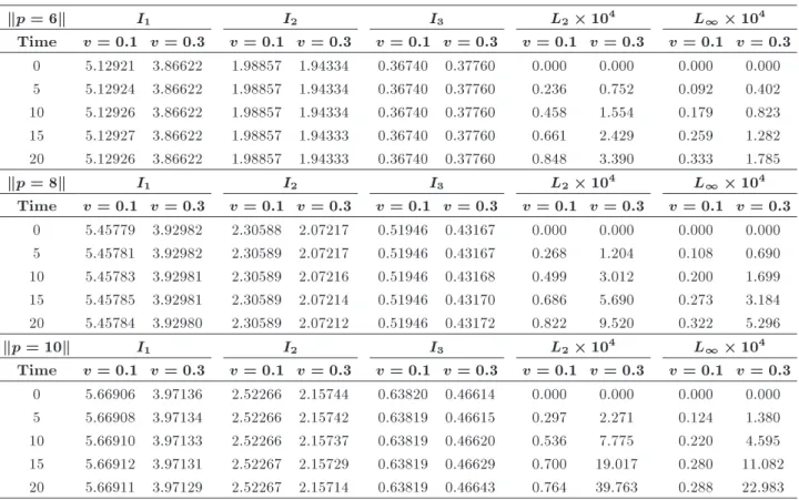
Table 2. Invariants and errors for Example 1 when x 2 [0; 100], h = 0:1, and t = 0:01.

kp = 6k I1 I2 I3 L2 104 _{L1 10}4

Time v = 0:1 v = 0:3 v = 0:1 v = 0:3 v = 0:1 v = 0:3 v = 0:1 v = 0:3 v = 0:1 v = 0:3 0 5.12921 3.86622 1.98857 1.94334 0.36740 0.37760 0.000 0.000 0.000 0.000 5 5.12924 3.86622 1.98857 1.94334 0.36740 0.37760 0.236 0.752 0.092 0.402 10 5.12926 3.86622 1.98857 1.94334 0.36740 0.37760 0.458 1.554 0.179 0.823 15 5.12927 3.86622 1.98857 1.94333 0.36740 0.37760 0.661 2.429 0.259 1.282 20 5.12926 3.86622 1.98857 1.94333 0.36740 0.37760 0.848 3.390 0.333 1.785

kp = 8k I1 I2 I3 L2 104 _{L1 10}4

Time v = 0:1 v = 0:3 v = 0:1 v = 0:3 v = 0:1 v = 0:3 v = 0:1 v = 0:3 v = 0:1 v = 0:3 0 5.45779 3.92982 2.30588 2.07217 0.51946 0.43167 0.000 0.000 0.000 0.000 5 5.45781 3.92982 2.30589 2.07217 0.51946 0.43167 0.268 1.204 0.108 0.690 10 5.45783 3.92981 2.30589 2.07216 0.51946 0.43168 0.499 3.012 0.200 1.699 15 5.45785 3.92981 2.30589 2.07214 0.51946 0.43170 0.686 5.690 0.273 3.184 20 5.45784 3.92980 2.30589 2.07212 0.51946 0.43172 0.822 9.520 0.322 5.296

kp = 10k I1 I2 I3 L2 104 _{L1 10}4

Time v = 0:1 v = 0:3 v = 0:1 v = 0:3 v = 0:1 v = 0:3 v = 0:1 v = 0:3 v = 0:1 v = 0:3 0 5.66906 3.97136 2.52266 2.15744 0.63820 0.46614 0.000 0.000 0.000 0.000 5 5.66908 3.97134 2.52266 2.15742 0.63819 0.46615 0.297 2.271 0.124 1.380 10 5.66910 3.97133 2.52266 2.15737 0.63819 0.46620 0.536 7.775 0.220 4.595 15 5.66912 3.97131 2.52267 2.15729 0.63819 0.46629 0.700 19.017 0.280 11.082 20 5.66911 3.97129 2.52267 2.15714 0.63819 0.46643 0.764 39.763 0.288 22.983

Table 3. Errors for Example 1 when x 2 [0; 100], = 1, and t = 20.

p = 2 p = 3 p = 4

v ! 0.03 0.1 0.3 0.03 0.1 0.3 0.03 0.1 0.3

amp ! 0.17 0.31 0.54 0.29 0.43 0.62 0.38 0.52 0.68

h t

L2 103

0.1 0.010 1.002 0.044 0.119 1.343 0.062 0.157 1.585 0.073 0.195 0.2 0.010 0.889 0.012 0.037 1.192 0.013 0.091 1.407 0.017 0.186 0.1 0.025 1.002 0.064 0.328 1.343 0.109 0.593 1.585 0.158 0.988 0.2 0.025 0.889 0.025 0.248 1.192 0.055 0.530 1.407 0.101 0.981 0.1 0.100 1.004 0.488 4.323 1.353 1.035 8.561 1.611 1.795 16.850 0.2 0.100 0.891 0.452 4.244 1.201 0.986 8.499 1.430 1.741 16.842

L1 103

0.1 0.010 0.403 0.014 0.051 0.541 0.022 0.072 0.638 0.027 0.095 0.2 0.010 0.403 0.006 0.017 0.541 0.007 0.043 0.638 0.007 0.091 0.1 0.025 0.403 0.023 0.143 0.541 0.042 0.277 0.638 0.064 0.482 0.2 0.025 0.403 0.009 0.105 0.541 0.022 0.245 0.638 0.042 0.475 0.1 0.100 0.403 0.199 1.894 0.541 0.433 4.016 0.638 0.766 8.235 0.2 0.100 0.403 0.185 1.854 0.541 0.414 3.984 0.638 0.744 8.213

Moreover, it is found that the magnitude of L2 and

L1 error norms is adequately small with increasing p,

time, and velocity, as expected.

Second, this study seeks to examine the quantity of error norms at dierent velocities, space steps, and

time steps. For this purpose, we have taken h = 0:1; 0:2, t = 0:01; 0:025; 0:1, and v = 0:03; 0:1; 0:3. The values of L2 and L1 error norms are listed at

t = 20 in Tables 3 and 4. In these tables, error norms are found to be small enough, and L1 error is always

Table 4. Errors for Example 1 when x 2 [0; 100], = 1, and t = 20.

p = 6 p = 8 p = 10

v ! 0.03 0.1 0.3 0.03 0.1 0.3 0.03 0.1 0.3

amp ! 0.52 0.63 0.76 0.60 0.70 0.81 0.66 0.75 0.84

h t

L2 103

0.1 0.010 1.900 0.084 0.339 2.094 0.082 0.952 2.225 0.076 3.976 0.2 0.010 1.686 0.049 0.699 1.858 0.158 2.887 1.974 0.521 13.291 0.1 0.025 1.901 0.296 2.954 2.095 0.590 12.175 2.228 1.461 57.247 0.2 0.025 1.686 0.268 3.316 1.859 0.679 14.108 1.976 1.926 66.443

L1 103

0.1 0.010 0.765 0.033 0.178 0.843 0.032 0.529 0.896 0.028 2.298 0.2 0.010 0.765 0.021 0.366 0.843 0.074 1.591 0.896 0.257 7.601 0.1 0.025 0.765 0.128 1.563 0.843 0.274 6.802 0.896 0.724 33.005 0.2 0.025 0.765 0.119 1.750 0.843 0.317 7.808 0.896 0.954 38.021

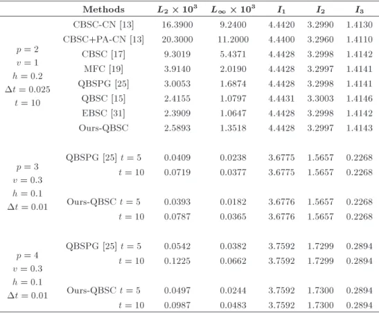
Table 5. Comparisons of results for Example 1 when x 2 [0; 100], and = 1.

Methods L2 103 _{L1 10}3 _{I1 I2 I3}

p = 2 v = 1 h = 0:2 t = 0:025

t = 10

CBSC-CN [13] 16.3900 9.2400 4.4420 3.2990 1.4130 CBSC+PA-CN [13] 20.3000 11.2000 4.4400 3.2960 1.4110 CBSC [17] 9.3019 5.4371 4.4428 3.2998 1.4142 MFC [19] 3.9140 2.0190 4.4428 3.2997 1.4141 QBSPG [25] 3.0053 1.6874 4.4428 3.2998 1.4141 QBSC [15] 2.4155 1.0797 4.4431 3.3003 1.4146 EBSC [31] 2.3909 1.0647 4.4428 3.2998 1.4142 Ours-QBSC 2.5893 1.3518 4.4428 3.2997 1.4143

p = 3 v = 0:3 h = 0:1 t = 0:01

QBSPG [25] t = 5 0.0409 0.0238 3.6775 1.5657 0.2268 t = 10 0.0719 0.0377 3.6775 1.5657 0.2268 Ours-QBSC t = 5 0.0393 0.0182 3.6776 1.5657 0.2268 t = 10 0.0787 0.0365 3.6776 1.5657 0.2268

p = 4 v = 0:3 h = 0:1 t = 0:01

QBSPG [25] t = 5 0.0542 0.0382 3.7592 1.7299 0.2894 t = 10 0.1225 0.0662 3.7592 1.7299 0.2894 Ours-QBSC t = 5 0.0497 0.0244 3.7592 1.7300 0.2894 t = 10 0.0987 0.0483 3.7592 1.7300 0.2894

smaller than L2 error. Here, it should be noted that

if the parameters h = 0:1, t = 0:01, and v = 0:1 are chosen, then L1 error norm remains less than

0:34 10 4 _{during the computer run.}

Table 5 reports that the obtained error norms are smaller than those obtained by other methods. In addition, three conservation laws are in agreement with the earlier works.

The behavior of a single solitary wave at dierent

time levels is plotted in Figure 1. Of note, the solitary wave keeps its identity and moves to the right at a constant velocity. By increasing p, a single solitary wave gathers greater energy.

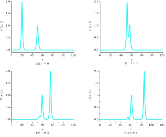
3.2. Example 2: The collision of two solitary waves

Consider the governing equation with the following initial condition, which is the linear sum of two well

Figure 1. The motion of a single solitary wave when x 2 [0; 100], v = 0:1, and x0= 40.

separated solitary waves with dierent amplitudes U(x; 0)

=X2

i=1 p

s

vi(p+2)

2p sec h2

p 2

r _v

i

(vi+1)(x xi)

;

(19) where viand xi, i = 1; 2, are arbitrary constants.

Numerical calculation is carried out under the following conditions: p = 2, x 2 [0; 250], h = 0:2, t = 0:025, = 1, v1= 4, v2= 1, x1 = 25, x2= 55,

p = 3, x 2 [0; 120], h = 0:1, t = 0:01, = 1, v1 = 48=5, v2 = 6=5, x1 = 20, x2 = 50, p = 4,

x 2 [0; 200], h = 0:125, t = 0:01, = 1, v1 = 64=3,

v2 = 4=3, x1 = 20, and x2 = 80. The computational

data are recorded in Tables 6 and 7, which denote that the quantities of the invariants change a little from their initial count, which are compatible with the results of the referenced paper [25]. The motion of two solitary waves is depicted at dierent time steps in Figures 2 and 3. As seen in these gures, at time zero, the solitary wave with larger energy is behind the second wave involving smaller energy. According to the solitary wave theory, greater energy means more velocity. Hence, over time, the large wave attains a smaller one and interposition takes place. Similarly, a wave with larger energy leaves behind the second wave with smaller energy, and the same is reiterated.

Table 6. Invariants for Example 2 when p = 2, x 2 [0; 250], h = 0:2, t = 0:025, = 1, v1= 4, v2= 1, x1= 25, and x2= 55.

I1 I2 I3

Time QBSC QBSPG QBSC QBSPG QBSC QBSPG

# Ours [25] Ours [25] Ours [25]

0 11.4676 11.4677 14.6292 14.6286 22.8803 22.8788 4 11.4676 11.4677 14.6277 14.6292 22.8818 22.8811 8 11.4668 11.4677 14.1399 14.6229 23.3695 22.8798 12 11.4676 11.4677 14.6803 14.6299 22.8292 22.8803 16 11.4676 11.4677 14.6442 14.6295 22.8653 22.8805 20 11.4676 11.4677 14.6309 14.6299 22.8786 22.8806

Table 7. Invariants for Example 2.

Time 0 1 2 3 4 5 6

p = 3

I1 9.6907 9.6894 9.6881 9.6851 9.6860 9.6848 9.6835 I2 12.9443 12.9433 12.9391 12.3044 12.9704 13.0539 13.0028 I3 17.0186 17.0197 17.0239 17.6586 16.9926 16.9091 16.9601

p = 4

I1 8.8342 8.6650 8.5662 8.4965 8.4529 8.4089 8.3702 I2 12.1708 11.9332 11.7919 11.6913 11.4644 11.7254 11.5990 I3 14.0294 14.2670 14.4083 14.5090 14.7358 14.4748 14.6012

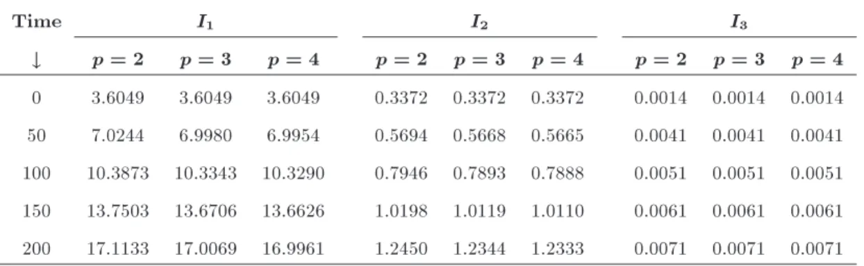
Table 8. Physical quantities for Example 3 when x 2 [ 36; 300], x0= 0, h = 0:1, t = 0:1, = 1=6, d = 5, and U0= 0:1.

Time I1 I2 I3

# p = 2 p = 3 p = 4 p = 2 p = 3 p = 4 p = 2 p = 3 p = 4 0 3.6049 3.6049 3.6049 0.3372 0.3372 0.3372 0.0014 0.0014 0.0014 50 7.0244 6.9980 6.9954 0.5694 0.5668 0.5665 0.0041 0.0041 0.0041 100 10.3873 10.3343 10.3290 0.7946 0.7893 0.7888 0.0051 0.0051 0.0051 150 13.7503 13.6706 13.6626 1.0198 1.0119 1.0110 0.0061 0.0061 0.0061 200 17.1133 17.0069 16.9961 1.2450 1.2344 1.2333 0.0071 0.0071 0.0071

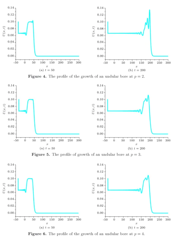
3.3. Example 3: Undular bore

Finally, we have worked on the growth of an undular bore:

U(x; 0) =1 2U0

1 tanh

x xc

d

; (20) which reects the elevation of the water surface above the equilibrium point. The change in the water level of magnitude Eq. (20) is centered on x = xc. To be

consistent with the papers [1,11,12], the parameters U0 = 0:1, = 1=6, h = 0:1, t = 0:1, xc = 0,

d = 5, and x 2 [ 36; 300] are used. The three

conservation laws are given in Table 8. From this table, it was observed that the change in the invariants was reasonably small. The undulation proles at dierent time steps are drawn in Figures 4 to 6. It can be concluded that the number of undulations increases when the value of x rises and waves move like this for a time. Afterwards, undulations take the peak position and disappear.

4. Conclusion

Figure 2. The collision of two solitary waves at p = 3.

Figure 4. The prole of the growth of an undular bore at p = 2.

Figure 5. The prole of growth of an undular bore at p = 3.

Figure 6. The prole of the growth of an undular bore at p = 4.

constructed for obtaining a numerical solution to the GRLW equation. Using the von-Neumann technique, the method was shown to be unconditionally stable. The QBSCM was tested with three examples including a single solitary wave, the collision of two solitary waves, and the growth of an undular bore. The error in L2, and L1norms and three conservative quantities I1,

I2, and I3 were calculated to conrm the performance

of the numerical scheme. The major point of the QBSCM is that it reduces the problem into a system of rst-order ordinary dierential equations. Then,

the system produces the recurrence relationship whose solutions can be found through the penta-diagonal system. Further to that, it is easy to apply the method to dierent values of " and p, which aect the nonlinear term, velocity, and initial condition. The ndings prove that three physical quantities of motion remain constant during wave propagation, and the results are the same as those of previous studies. The magnitude of the obtained error norms is adequately small, and it is better than the ones in earlier works. Hereby, the proposed scheme is a practical, accurate and powerful

numerical technique. It can be condingly used for solving similar types of nonlinear problems.

Acknowledgements

The authors are very grateful to anonymous referees for their detailed reading, precious comments, and proposals.

References

1. Peregrine, D.H. \Calculations of the development of an undular bore", Journal of Fluid Mechanics, 25, pp. 321-330 (1966).

2. Peregrine, D.H. \Long waves on a beach", Journal of Fluid Mechanics, 27, pp. 815-827 (1967).

3. Benjamin, T.B., Bona, J.L., and Mahony, J.J. \Model equations for long waves in non-linear dispersive sys-tems", Philosophical Transactions of the Royal Society of London Series A, 272, pp. 47-78 (1972).

4. Morrison, P.J., Meiss, J.D., and Carey, J.R. \Scatter-ing of RLW solitary waves", Physica D, 11, pp. 324-336 (1984).

5. Raslan, K.R. \Collocation method using quadratic B-spline for the RLW equation", International Journal of Computer Mathematics, 78, pp. 399-412 (2001).

6. Dag, I., Saka, B., and Irk, D. \Application of cubic B-splines for numerical solution of the RLW equation", Applied Mathematics and Computation, 159(2), pp. 373-389 (2004).

7. Saka, B., Dag, I., and Irk, D. \Quintic B-spline collocation method for numerical solution of the RLW equation", The ANZIAM Journal, 49(3), pp. 389-410 (2008).

8. Saka, B., Sahin, A., and Dag, I. \B-spline colloca-tion algorithms for numerical solucolloca-tion of the RLW equation", Numerical Methods for Partial Dierential Equations, 27, pp. 581-607 (2011).

9. Soliman, A.A. and Hussien, M.H. \Collocation solu-tion for RLW equasolu-tion with septic spline", Applied Mathematics and Computation, 161(2), pp. 623-636 (2005).

10. Dag, I., Saka, B. and Irk, D. \Galerkin method for the numerical solution of the RLW equation using quintic B-splines", Journal of Computational and Applied Mathematics, 190, pp. 532-547 (2006).

11. Esen, A. and Kutluay, S. \Application of a lumped Galerkin method to the regularized long wave equa-tion", Applied Mathematics and Computation, 174, pp. 833-845 (2006).

12. Mei, L. and Chen, Y. \Numerical solutions of RLW equation using Galerkin method with extrapolation techniques", Computer Physics Communications, 183, pp. 1609-1616 (2012).

13. Gardner, L.R.T., Gardner, G.A., Ayoub, F.A., and Amein, N.K. \Approximations of solitary waves of the MRLW equation by B-spline nite element", Arabian Journal for Science and Engineering, 22, pp. 183-193 (1997).

14. Haq, F., Islam, S., and Tirmizi, I.A. \A numerical technique for solution of the MRLW equation using quartic B-splines", Applied Mathematical Modelling, 34(12), pp. 4151-4160 (2010).

15. Karakoc, S.B.G., Yagmurlu, N.M., and Ucar, Y. \Numerical approximation to a solution of the mod-ied regularized long wave equation using quintic B-splines", Boundary Value Problems, 2013, pp. 1-17 (2013).

16. Karakoc, S.B.G., Ak, T., and Zeybek, H. \An ecient approach to numerical study of the MRLW equation with B-spline collocation method", Abstract and Ap-plied Analysis, 2014, pp. 1-15 (2014).

17. Khalifa, A.K., Raslan, K.R., and Alzubaidi, H.M. \A collocation method with cubic B-splines for solving the MRLW equation", Journal of Computational and Applied Mathematics, 212, pp. 406-418 (2008).

18. Raslan, K.R. and EL-Danaf, T.S. \Solitary waves solutions of the MRLW equation using quintic B-splines", Journal of King Saud University - Science, 22(3), pp. 161-166 (2010).

19. Ali, A. \Mesh free collocation method for numerical so-lution of initial-boundary value problems using radial basis functions", Ph.D. Thesis, Ghulam Ishaq Khan Institute of Engineering Sciences and Technology, Pak-istan (2009).

20. Dag, I., Irk, D., and Sari, M. \The extended cubic B-spline algorithm for a modied regularized long wave equation", Chinese Physics B, 22(4), pp. 1-6 (2013).

21. Abo Essa, Y.M., Abouefarag, I., and Rahmo, E.-D. \The numerical solution of the MRLW equation using the multigrid method", Applied Mathematics, 5, pp. 3328-3334 (2014).

22. Bona, J.L., McKinney, W.R., and Restrepo, J.M. \Stable and unstable solitary-wave solutions of the generalized regularized long-wave equation", Journal of Nonlinear Science, 10, pp. 603-638 (2000).

23. Hammad, D.A. and El-Azab, M.S. \A 2N order compact nite dierence method for solving the gen-eralized regularized long wave (GRLW) equation", Applied Mathematics and Computation, 253, pp. 248-261 (2015).

24. Huang, D.M. and Zhang, L.W. \Element-free approxi-mation of generalized regularized long wave equation", Mathematical Problems in Engineering, 2014, pp. 1-10 (2014).

25. Mokhtari, R. and Mohammadi, M. \Numerical so-lution of GRLW equation using Sinc-collocation method", Computer Physics Communications, 181, pp. 1266-1274 (2010).

26. Roshan, T. \A Petrov-Galerkin method for solving the generalized regularized long wave (GRLW) equation", Computers and Mathematics with Applications, 63, pp. 943-956 (2012).

27. Soliman, A.A. \Numerical simulation of the general-ized regulargeneral-ized long wave equation by He's variational iteration method", Mathematics and Computers in Simulation, 70, pp. 119-124 (2005).

28. Zhang, L. \A nite dierence scheme for generalized regularized long-wave equation", Applied Mathematics and Computation, 168, pp. 962-972 (2005).

29. Kaya, D. and El-Sayed, S.M. \An application of the decomposition method for the generalized KdV and RLW equations", Chaos, Solitons and Fractals, 17, pp. 869-877 (2003).

30. Hamdi, S., Enright, W.H., Schiesser, W.E., and Got-tlieb, J.J. \Exact solutions and invariants of motion for general types of regularized long wave equations", Mathematics and Computers in Simulation, 65, pp. 535-545 (2004).

31. Ramos, J.I. \Solitary wave interactions of the GRLW equation", Chaos, Solitons & Fractals, 33, pp. 479-491 (2007).

32. Mohammadi, R. \Exponential B-spline collocation method for numerical solution of the generalized reg-ularized long wave equation", Chinese Physics B, 24, pp. 1-14 (2015).

33. Zeybek, H. and Karakoc, S.B.G. \A numerical investi-gation of the GRLW equation using lumped Galerkin approach with cubic B-spline", SpringerPlus, 5, pp. 1-17 (2016).

34. Karakoc, S.B.G. and Zeybek, H. \Solitary-wave so-lutions of the GRLW equation using septic B-spline collocation method", Applied Mathematics and Com-putation, 289, pp. 159-171 (2016).

35. Irk, D. and Dag, I. \Quintic B-spline collocation method for the generalized nonlinear Schrodinger equation", Journal of the Franklin Institute, 348, pp. 378-392 (2011).

36. Ismail, M.S. \Numerical solution of complex modied Korteweg-de Vries equation by collocation method", Communications in Nonlinear Science and Numerical Simulation, 14, pp. 749-759 (2009).

37. Mittal, R.C. and Tripathi, A. \Numerical solutions of generalized Fisher and generalized Burgers-Huxley equations using collocation of cubic B-splines", International Journal of Computer Mathematics, 93, pp. 1053-1077 (2015).

38. Ak, T., Karakoc, S.B.G., and Biswas, A. \Application of Petrov-Galerkin nite element method to shallow water waves model: modied Korteweg-de Vries equa-tion", Scientia Iranica, 24, pp. 1148-1159 (2017).

39. Prenter, P.M., Splines and Variational Methods, J. Wiley, New York (1975).

40. Rubin, S.G. and Graves, R.A., A Cubic Spline Approx-imation for Problems in Fluid Mechanics, NASA TR R-436, Washington, DC (1975).

Biographies

Halil Zeybek graduated from Ondokuz Mays Uni-versity in 2008 with a BSc degree in Mathematics. He received his MSc and PhD degrees in Applied Math-ematics from Nevsehir Hac Bektas Veli University in 2011 and 2016, respectively. He is currently a Research Assistant in Abdullah Gul University. He has done his research and publications in the areas of solitary waves, uid dynamics, numerical analysis, and applied mathematics.

Seydi Battal Gazi Karakoc graduated from Selcuk University in 2001 with a BSc degree in Mathematics. He received his MSc and PhD degrees in Applied Mathematics from _Inonu University in 2006 and 2011, respectively. He is currently an Assistant Professor in Nevsehir Hac Bektas Veli University. He has done his research and publications in the areas of nite element method, numerical simulation, and applied mathematics.