Effects of Sample Size Ratio on the Performance of the Quadratic Discriminant Function

(1)

EFFECTS OF SAMPLE SIZE RATIO ON THE

PERFORMANCE OF THE QUADRATIC DISCRIMINANT

FUNCTION

A. ADEBANJI1_{, S. NOKOE}2_{AND S. ADEYEMI}3

1_{Department of Mathematics, Kwame Nkrumah University of Science and Technology,}

2_{Department of Applied Mathematics and Computer Science, University for}

Development Studies, Navrongo, Ghana. Email: [email protected]. 3_{Tibotec-Virco BVBA, Belgium.}_Email_{: [email protected]}

_pxp. The ith group conditional density fi(Xi,

θi) is given by

ABSTRACT

This study investigated the performance of the heteroscedastic discriminant function under the non-optimal condition of unbalanced group representation in the populations. The asymptotic performance of the classification function with respect to increased Mahalanobis’ distance (under this condition) was considered. Results obtained have shown that the misclassification of observations from the smaller group escalates when the sample size ratio 1:2 is exceeded (for small sample sizes). Results also show more sensitivity to sample size than the distance function when the data set is balanced, while the performance of the function in the classification of the underrepresented group improved by increasing the distance function. More robustness with unbalanced data was also observed with the Quadratic Function than the Linear Discriminant Function.

Keywords: Heteroscedastic, Unbalanced data, Discriminant function, prior probabilities,

Misclassification 2000 Mathematics Subject Classification: 62H30, 62C05, 00A72.

INTRODUCTION

In this study we restrict ourselves to the two group classification problem when the covariance structures and mean vectors are unequal. We define two groups R1 and R2 with Multivariate Normal density functions

f1(x) and f2(x) respectively. R1 ׽ Np(μ1,Σ1) and R2 ׽ Np(μ2,Σ2)where μi א _p and Σi א

……….. (1.1)

Journal of Natural Sciences, Engineer-ing and Technology ISSN- 2277 - 0593

(2)

and θi consists of the elements of μi and the (1/2)P(P + 1) distinct elements of Σi (i =1, ..., g). It is assumed that each Σi is nonsingular. The elements of the vector P of the mix-ing proportions for the populations sum up to 1.

Observations from these groups constitute the training sample. A classification function will be constructed using the training sample on the basis of which future observations (of unknown group memberships) will be classified. This is done by comparing the function to a predetermined cut-off value. The procedure is often utilized (but not limited to) the Social Sciences, Medical sciences, Education and Psychology.

MATERIALS AND METHODS

The Model

The optimal discriminant rule that minimizes the total probability of misclassification is given by the log ratio of densities. That is:

(2.1) This reduces to:

(2.2) This is a quadratic classification function here after referred to as the Quadratic Discrimi-nant

Function (QDF). This function contains population parameters and the sample estimates will be obtained from the training data. is the general equation. Equation (2.2) above can be written as

Q(x) = x/_Ax₊_b/_x₊_c_(2.3)

where

(2.4)

The quadratic

(2.5)

(3)

is the squared Mahalanobis’ distance between x and μi with respect to Σ.

The cut-off point is determined by the log ratios of the costs of misclassification and prior probabilities. We define as the cost of misclassifying an observed vector as belonging to group Ri when it actually belongs to Rj and C(j|i) as the converse.

Consequently, C(i|i) = C(j|j) = 0. Also, the assumption C(j|i) = C(i|j) is the exception and not the norm in practice. This rule is however regularly applied when the misclassification costs are unknown.

Let Pi i=1, 2 be the prior probability of an observation belonging to group Ri and this

in-formation is often obtained from the training sample composition. An observed P-variate vector x is assigned to R1 if

(2.6)

The total probability of misclassification (TPM) gives a measure of the performance of the function. This is a proportion of misclassified observations from the training sample and is given as:

(2.7)

Denote where and are the distributions that generated the

train-ing samples, the TPM ustrain-ing the QDF will be represented as

(2.8)

where

A(R0_{) = (1}_/₂₎₍_C₂₍_R0₎-1_{– C}₁₍_R0₎-1₎ _(2.9)

b(R0_{) =}_C₁₍_R0₎-1_T₁₍_R0₎-1_{– C}₂₍_R0₎-1_T₂₍_R0₎-1 _(2.10) c(R0_{) = (1}_/_2)log(|_C₂₍_R0_)||_C₁₍_R0_{)| +(1}_/₂₎₍_T₂₍_R0₎/_C₂₍_R0₎-1_T₂₍_R0₎

− T1(R0)/C1(R0)-1T1(R 0)) (2.11)

This is analogous to the quadratic function and equations 2.9 to 2.11 are the values of a lo-cation function T at the distributions and .

That is, and Similarly, C1(R0) and C2(R0) are the

(4)

Thus, and When the data follow a normal distribution,

T1(R0) = μ1, T2(R0) = μ2, C1(R0) = Σ1 and C2(R0) = Σ2 (Joossens(5)).

McFarland and Richards(7) have provided exact misclassification probabilities for the finite sample from a normal distribution. The future data are supposed to be a normal mixture of the training data and the observations of unknown group membership. This gives a TPM for the mixture as

TPM(R0_{, R}_{) =}_P₁_C_(2|1)(_R0_{, R}_{) +}_P₂_C₍₁_|₂₎₍_R0_{, R}₎_(2.12)

The theoretical derivations have been provided by Jossens(5), McFarlan and Richards (7) and McLachlan (8).

The Simulation Experiment

We consider two populations R1׽ N

(μ4,Σ4x4) and R2 (μ4,Σ4x4) with

μ1 =(0,0,0,0) and μ2 = (δ,0,0,0), Σ1 =I and

Σ2 = kI. For our case we set k=6 (Adebanji and Nokoe(1)) and δ=1, 2, 3 and 4. Differ-ent values of δare considered to see if there is any observable change in the perform-ance of the functions from very close sam-ples to well separated samsam-ples. Twenty one sample sizes (ranging from 25 to 500) are generated for R1 and the number of corre-sponding observations generated from R2 is determined by the sample size ratio compo-sition under consideration. We consider n1 : n2 = 1:1, 1:2, 1:3 and 1:4; that is from

bal-anced to extremely unbalbal-anced data sets. The large sample sizes are considered in order to enable us observe the performance of the QDF when the population parame-ters are known.

The four sample size ratio combinations are considered for every value of δunder con-sideration. Random samples are generated and 100 replications of each sample

specifi-The large number of replications minimizes between sample variability. The QDF is con-structed and the leave-one-out error rate esti-mation procedure (Lachembruch and Mickey (6))is used for estimating the TPM.

Results of Simulation

In the results, the total probability of mis-classification (averaged over 100 replications) is denoted as decimals, and the associated standard deviations (SD) are also denoted as decimals. The coefficient of variation (CV) (denoted as percentages) are presented. Re-sults are also presented for different values of δand sample size ratio combinations.

Scheme 1: Equal Sample sizes (n1:n2=1:1)

When the sample size ratios are equal, the performance of the function for group G1

with an identity covariance structure is

slightly better than that for G2 with the

co-variance structure Σ=kI though not signifi-cantly different in values. Higher reduction in error rates and SD was observed for in-creased sample sizes than for increase in

(5)

cant improvement was recorded in the per-formance of the function.

Scheme 2: Unequal Sample sizes (n1 :

n2=1:2)

The ratio of the error rates for G2: G1 was

1:5 and this increased to 1:10 when the sample size 1200 was attained for δ=1. This high misclassification of the under-represented group underscored the im-provement in the performance of the func-tion as can be observed from the total error

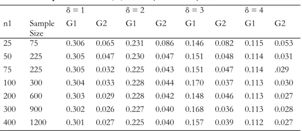
rates. The SD shows a steady decline to sam-ple size 900 at which it stabilizes. The CV reduces more gradually to sample size 1200 and remained stable afterwards. For δ=2, the ratio was 1:3 for smaller sample sizes and 1:6 when the sample size 1200 was attained. For δ=3, the ratio increased to 1:4 and similar results was observed for δ=4. The group er-ror rates for this scheme are presented in Table 1.

Table 1: Group Error for δ = 1, 2, 3 and 4(n1:n2 = 1 : 2)

δ = 1 δ = 2 δ = 3 δ = 4

n1 Sample

Size G1 G2 G1 G2 G1 G2 G1 G2

25 75 0.306 0.065 0.231 0.086 0.146 0.082 0.115 0.053

50 225 0.305 0.047 0.230 0.047 0.151 0.048 0.114 0.031

75 225 0.305 0.032 0.225 0.043 0.151 0.047 0.114 .029

100 300 0.304 0.033 0.228 0.044 0.170 0.037 0.113 0.030

200 600 0.303 0.029 0.228 0.042 0.148 0.046 0.113 0.027

300 900 0.302 0.026 0.227 0.040 0.168 0.036 0.113 0.028

400 1200 0.301 0.027 0.225 0.040 0.157 0.039 0.112 0.027

Scheme 3:Unequal Sample sizes (n1 :

n2=1:3)

The ratio of the error rates G2 : G1 for δ= 1 increased from 1:9 to 1:26 at sample size 1200, for δ= 2, it rose from 1:4 to 1:9. At δ = 3, the change was from 1:4 to 1:6 and 1:2 to 1:4 for δ= 4. The high error rate for the smaller group further underscores the per-formance of the function. There was a steady reduction in the SD until sample size 800 beyond which it remained relatively constant. A similar pattern was observed for the CV which recorded only a slight

im-provement beyond sample size 800. Refer to Table 2 below for the group error rates.

Scheme 4:Unequal Sample sizes (n1 :

n2=1:4)

The widening in the gap of the ratio G2:G1

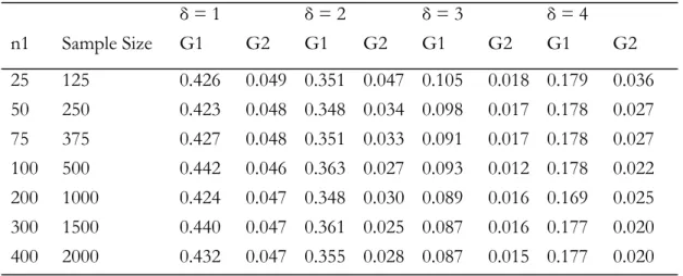
was not as rapid as had earlier been ob-served. For δ= 1 the increase was from 1:9 to 1:11, while for δ= 2, 3 and 4 the recorded values were 1:4 to 1:7, 1:6 to 1:8 and 1:5 to 1:9 respectively. See Table 3 below for de-tails of change in error rates.

(6)

Table 2: Group Error for δ = 1, 2, 3 and 4(n1 : n2=1:3)

δ = 1 δ = 2 δ = 3 δ = 4

n1 Sample Size G1 G2 G1 G2 G1 G2 G1 G2

25 100 0.412 0.043 0.279 0.065 0.193 0.054 0.139 0.046

50 200 0.412 0.027 0.283 0.045 0.195 0.054 0.135 0.033

75 300 0.411 0.018 0.284 0.042 0.195 0.044 0.133 0.029

100 400 0.410 0.020 0.299 0.036 0.205 0.038 0.127 0.032

200 800 0.410 0.016 0.280 0.040 0.193 0.039 0.125 0.032

300 1200 0.409 0.016 0.297 0.031 0.204 0.035 0.122 0.031

400 1600 0.409 0.016 0.288 0.035 0.198 0.034 0.084 0.044

Table 3: Group Error for δ = 1, 2, 3 and 4(n1 : n2=1:4)

δ = 1 δ = 2 δ = 3 δ = 4

n1 Sample Size G1 G2 G1 G2 G1 G2 G1 G2

25 125 0.426 0.049 0.351 0.047 0.105 0.018 0.179 0.036

50 250 0.423 0.048 0.348 0.034 0.098 0.017 0.178 0.027

75 375 0.427 0.048 0.351 0.033 0.091 0.017 0.178 0.027

100 500 0.442 0.046 0.363 0.027 0.093 0.012 0.178 0.022

200 1000 0.424 0.047 0.348 0.030 0.089 0.016 0.169 0.025

300 1500 0.440 0.047 0.361 0.025 0.087 0.016 0.177 0.020

400 2000 0.432 0.047 0.355 0.028 0.087 0.015 0.177 0.020

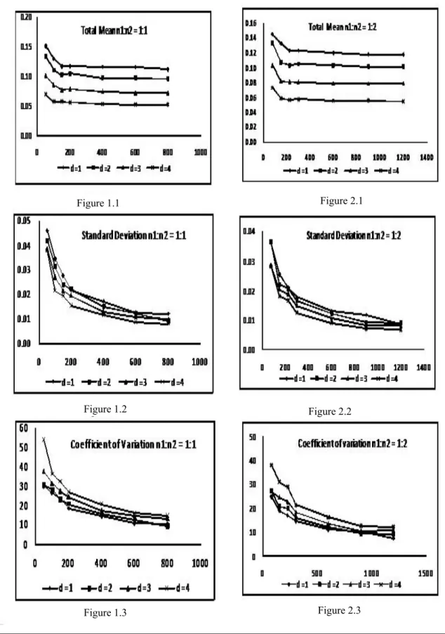
Mean Error rates, SD and CV

The graphs for the total (mean) error rates, standard deviation (SD) and coefficient of variation are presented in a series of Figures 1.1 to 4.3. Figures 1.1, 1.2 and 1.3 are the graphs of the mean error rates, SD and CV for the balanced data set. Figures 2.1, 2.2 and 2.3 represent the mean error rates, SD and CV for sample size composition n1 : n2=1:2. The graphs for sample size ratios

1:3 and 1:4 are presented in Figures 3.1 to 3.3 and 4.1 to 4.3 respectively.

DISCUSSION

When the data set is balanced, the QDF benefits more from increase in sample size than increase in the distance function. More robustness was also observed in using the function for unbalanced data over the linear discriminant function (Adebanji et al.) (2). The performance of the function in classify-ing unbalanced data also improved signifi-cantly when the between group squared dis-tance is relatively large (i.e data sets are well separated). The performance, however, dete-riorates in classifying the smaller group when

(7)

Figure 1.1 Figure 2.1

Figure 1.2 _{Figure 2.2}

(8)

Figure 3.1

Figure 3.2

Figure 3.3

Figure 4.1

Figure 4.2

(9)

CONCLUSION

In conclusion, using the QDF for the classi-fication of unbalanced data will not be rec-ommended beyond sample size ratio 1:2 when the data sets are relatively close, and ratio 1:3 when the observations are well separated (subject to moderate sample size).

REFERENCES

Adebanji, A.O., Nokoe Sagary, S.K.

2004. Evaluating the Quadratic Classifier, Proceedings of the Third International Workshop on contemporary problems in Mathematical Physics, 3: 369-394.

Adebanji, A.O., Adeyemi, S., Iyaniwura, O. Effects of sample size ratio on the Lin-ear Discriminant Function, International Jour-nal of Modern Mathematics, 3(1): 97-108.

http://ijmm.dixiewpublishing.com/

Fisher, R.A. 1936. The Use of Multiple Measurements in Taxonomic Problems,

Annals of Eungenics, 7: 179-188.

Fisher, R.A. 1938. Statistical Utilization of

Multiple Measurements, Annals of Eugenecs 8,

376-386.

Joossens, K. 2006. Robust Discriminant Analysis, Ph.D. Thesis of the Katholieke Uni-versity, Leuven, Belgium, 31-46.

Lachenbruch, P.A., Mickey, M.R. 1968. Estimation of error rates in discriminant analysis, Technometrics, 10:1-11.

McFarlan, R.H. Richards, D. 2002. Ex-act Misclassification Problems for Plug-in Normal Discriminant Functions: The Het-erogeneous Case, Journal of Multivariate Analy-sis, 82: 229-330.

McLachlan, G.A 1992. textbook of Discrimi-nant Analysis and Statistical Pattern Recognition, Wiley Series in Probability and Mathematical Statistics.

Murray, G.D. 1977. A Cautionary Note on Selection of Variables in Discriminant Analy-sis, Applied Statistics, 26(3): 246-250.