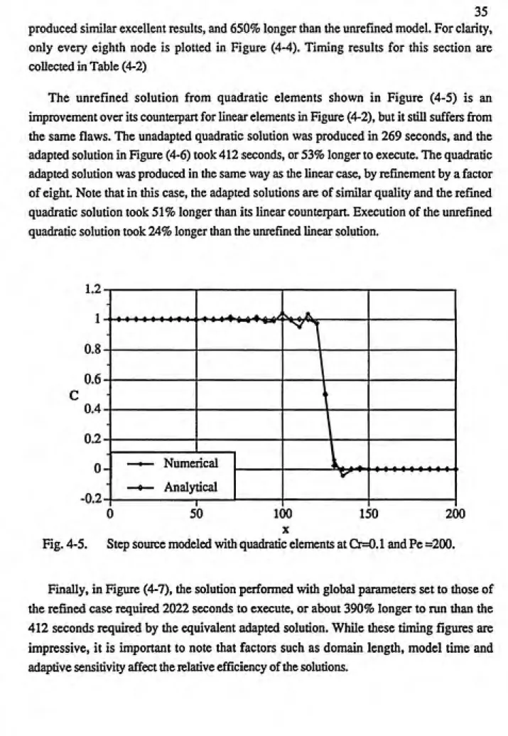
FRANK H. CORNEW. An Analysis of Methods for Accurate Modeling of Advective-Dominated Transport (Under the direction of CASS T. MILLER.)
Finite element modeling of sharp front advective-dispersive-reactive transport is not accurate for highly advective or reactive problems. Two techniques were studied with the goal of accurately modeling these problems: an /i-adaptive method that adjusted element lengths, and Petrov-Galerkin upwinding which used weighting functions of higher polynomial order than that of the basis functions.
Finite element models were constructed using linear and quadratic basis functions in one spatial dimension. The /i-adaptive method was shown to give good results with linear and quadratic basis functions. Petrov-Galerkin upwinding also yielded excellent results. This method was implemented for both classes of basis functions, but was studied only for
the linear case.
The benefits of Petrov-Galerkin upwinding depend on user defined parameters that regulate the amount of upwinding applied to the solution. Taylor series and Fourier analyses of the finite element truncation error as well as numerical experimentation were performed to define optimal upwinding parameters. Published results by other investigators were reproduced, and an automated method of deriving optimal upwinding parameters was
developed.
Analysis and operation of the Petrov-Galerkin models indicated that optimal levels of upwinding are a function of the gradient across each element. This observation led to a new upwinding scheme that adjusts the upwinding condition at each element as a function of the local gradient. Significantly better results were obtained with the new method relative to existing Petrov-Galerkin formulations.
The utility of this technique will be greatly enhanced when optimal upwinding conditions are described as a function of dimensionless model parameters such as P6clet, Courant, and Damkohler numbers, and the method is generalized to multiple spatial
Acknowledgment
This work would not have been possible with out the help of my parents, Richard and Chrystel Comew, my advisor. Dr. Casey Miller, and Beverly Brooks. The patience and support exhibited by all of these individuals is gready appreciated. Furthermore, I thank Dr. Andrew Balber for general professional advice and inspiration, and Elizabeth Nelson for technical assistance. C.L. Lassiter and Donna Simmons have provided valuable administrative support for which I am grateful.
TABLE OF CONTENTS
Page
LIST OF FIGURES...v
LIST OF TABLES...viii
ABBREVIATIONS...ix
NOTATION...X 1 INTRODUCTION...1
2 BACKGROUND AND LITERATURE REVIEW...4
2.1 Modeling...4
2.2 Numerical Models...5
2.2.1 Lagrangian Methods...5
2.2.2 Eulerian Methods...6
2.2.3 Matrix Solution Techniques...9
2.2.4 Upwinding...10
2.2.4.1 Petrov-Galerkin Upwinding...10
2.2.4.2 Weighting Functions...11
2.2.4.3 Optimal Upwinding Parameters...11
2.2.4.4 Two Dimensional Implementation...12
2.2.4.5 Variants...14
2.2.4.6 Applications...14
2.2.5 Adaptive Methods...15
2.2.5.1 Error Evaluation...15
2.2.5.2 Algorithms...16
3 MODEL DEVELOPMENT AND VALIDATION...20
3.1 Finite Element Formulation...20
3.2 Basis and Weighting Functions...22
3.3 Coefficient matrices...26
3.4 Adaptive Method...27
3.5 Validation...29
3.6 Features...31
3.7 Computing Environment...31
4 MATHEMATICAL ANALYSIS AND RESULTS...32
4.1 Adaptive Method Results...32
4.2 Petrov Galeikin Upwinding Analysis and Results...40
4.2.1 Taylor Series Analysis...43
4.2.2 Fourier Analysis...56
4.2.3 Numerical Experimentation...57
5 GRADIENT UPWINDING...67
5.1 Motivation...67
5.2 Formulation...67
5.3 Results...71
6 CONCLUSIONS AND RECOMMENDATIONS...79
6.1 Uniform upwinding...80
6.2 Gradient upwinding...81
LIST OF FIGURES
Page
2-1. Floating nodes in 2-D grid refinement...18
=00. 3-1. Dispersion and oscillation in a finite element solution at Cr=0.24, Pe=o
and lOOtimesteps...20 3-2. (a) Linear basis functions (b) Quadratic modifying function (c) Cubic
modifying function...23 3-3. Weighting functions from linear basis functions and N+2 degree
upwinding: a=l, p=l...23 3-4. (a) Quadratic basis functions (b) Cubic modifying function (c) Quartic
modifying function...25 3-5. Weighting functions from quadratic basis functions with: (a) N+1 degree
upwinding: ac=a^=l, Pc=Pm=0, (b) N+2 degree upwinding: occ=am=0,
Pc=Pm=^ (c) N+1 and N+2 degree upwinding: ac=0Wi=l, Pc=^m=i...25
3-6. Node numbering used for unrefined global elements and a refined
element...28
3-7. Refined element submatrix composed with numbering from Figure (3-6)...29
3-8. (a) Reduced refined element matrix and (b), the common area shared with
Ae global matrix...30
4-1. Step source for adaptive examples...33 4-2. Step source modeled with linear elements at Cr=0.1 and Pe =200...33 4-3. Step source modeled with adapted linear elements. The refined elements
indicated with shading have Q=0.8 and Pe=25, while the unrefined
elements have Cr=0.1 and Pe=200...34
4-4. Step source modeled with linear elements at Cr=0.8 and Pe =25...34 4-5. Step source modeled with quadratic elements at Cr=0.1 and Pe =200...35 4-6. Step source modeled with adapted quadratic elements. The refined
elements indicated with shading have Cr=0.8 and Pe=25, while Cr=0.1 and
Pe=200 for unrefined elements...36
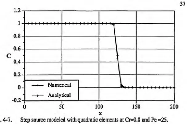
4-7. Step source modeled with quadratic elements at Cr^.8 and Pe =25...37
4-8. Gaussian source modeled with linear elements at Cr=0.1 and Pe=200...38
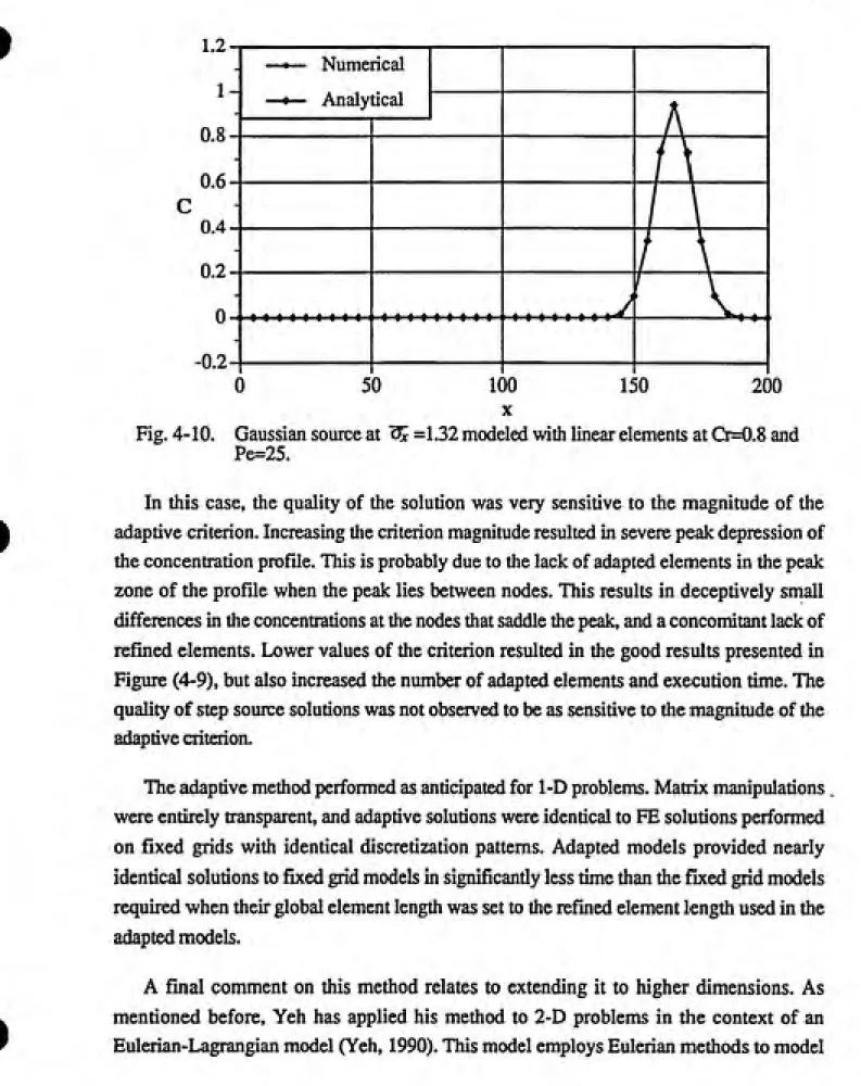
4-9. Gaussian source at <3J =1.32 modeled with adapted linear elements. The refined elements indicated with shading have Cp=0.8 and Pe=25, while
Cr=0.1 and Pe=200 for unrefined elements...38 4-10. Gaussian source at <^ =1.32 modeled with linear elements at Cr=0.8 and
Pe=25...39
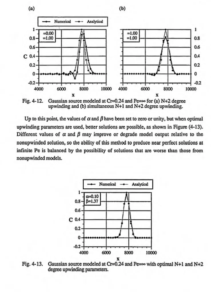
4-11. Gaussian source modeled at Cr=0.24 and Pe=<» for (a) no upwinding and (b) N+1 degree upwinding...41 4-12. Gaussian source modeled at Cr=0.24 and Pe=«> for (a) N+2 degree
#
4-13. Gaussian source modeled at Cr=0.24 and Pe=o° with optimal N+1 and
N+2 degree upwinding parameters...42
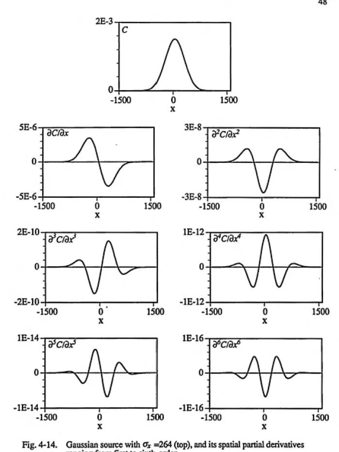
4-14. Gaussian source with <yx =264 (top), and its spatial partial derivatives
ranging from first to sixth-order...48
4-15. Seventh- through tenth-order partial derivatives of a Gaussian source with Ox =264...49
4-16. Fid'C'dx' terms from third- to tenth-order of a Gaussian source with
^ =1.32, Pe=oo, and Cr=0.24...50
4-17. Observed truncation error compared to the error predicted by a tenth-order Taylor series expansion. Model of a Gaussian source with "^ =1.32,
Pe=«>, and Cr=0.24 after one timestep...51 4-18. Truncation error of a Gaussian source with ^ =0.50, Pe=oo, and
Cr=0.24. over one timestep. Comparison of the observed error with: (a) Error predicted by a tenth-order Taylor series expansion, (b) Error
predicted by fifteenth-order Taylor series expansion...52
4-19. Fid'Cidx' terms from third to tenth-order of a Gaussian source with
^ =0.50, Pe=oo, and Cr=0.24...53
4-20. Observed tmncation error compared to the error predicted by a
fifteenth-order Taylor series expansion. Model of a Gaussian source with ^ =1.32, Pe=oo, and Cr=0.80 over one timestep...54
4-21. BG model of a Gaussian source with ^ =1.32, Pe=oo, and Cr=0.8, after
30 timesteps. 0=0.0000, ^3=0.0000...58
4-22. PG model of a Gaussian source with ^ =1.32, Pe=oo, and Cr=0.8, after
30 timesteps. op=0. 1000, and )3=1.3700 from Westerink and Shea
(1989)...59
4-23. PG model of a Gaussian source with ^ =1.32, Pe=oo, and Cr=0.8, after
30 timesteps. o^.Ol 13, and j3=1.3812 from LMDIFl...62
4-24. PG model of a Gaussian source with ^ =1.00, Pe=oo, and Cr=0.8, after
30 timesteps. 0=0.1000, and )3=1.3700 from Westerink and Shea
(1989)...62
4-25. BG model of a Gaussian source with ^ =1.32, Pe=oo, and Cr=0.8, after
100 timesteps. 0=0.0000 and j3=0.0000...63
4-26. PG model of a Gaussian source with ^ =1.32, Pe=«», and Cr=0.8, after
100 timesteps. o=0.1000,and /3=1.3700 from Westerink and Shea
(1989)...63
4-27. PG model of a Gaussian source with ^ =1.32, Pe=oo, and Cr=0.8, after
100 timesteps. o=0.0113, and j3=1.3812 from LMDIFl...64
4-28. PG model of a Gaussian source with HZ =1,00, Pe=oo, and Cr=0.8, after
100 timesteps. as=0.1000, and j3=1.3700 from Westerink and Shea
(1989)...64 4-29. Contour plot of Ed as a function of o and /3 for a Gaussian source with
^ =0.66, Pe=«», and Cr=0.24 after 1 timestep...65 4-30. Contour plot of Ed as a function of o and p for a Gaussian source with
^ =1.32, Pe=oo, and Cr=0.24 after 1 timestep...65 4-31. Contour plot of Ed as a function of a and )3 for a Gaussian source with
5-1. Analytical solution of a Gaussian source described by Table (5-1) with
^ =1.00, Pe=106 and Cr=0.8...70
5-2. Gradient upwind weighting functions that correspond to elements
indicated by (a), (b), and (c) in Figure (5-1)...70
5-3. Uniformly upwinded model of a Gaussian source with ^ =1.32, Pe=10^,
and Cr=0.8, after 100 timesteps. Optimized for ^ =1.32 with ct^.Ol 13, and y3=1.3812 from LMDIFl...72
5-4. GU model of a Gaussian source with m =1.32, Pe=106, and Cr=0.8, after
100 timesteps. Optimized with 1< ^ <4 in 0.01 increments. ab=0.03480,
ai=0.22025, A)=l-38410, and ^=-000452...73
5-5. GUmodelof a Gaussian source with ^=1.32, Pe=106, and Cr=0.8, after 100 timesteps. Optimized for (JJ =1.32 with Qb=0.03186, ai=0.16249,
A)=l.36040, and i3i=0.00487...73
5-6. GU model of a Gaussian source with ^ =1.00, Pe=106, and Cr=0.8, after 100 timesteps. Optimized with 1< ^ <4 in 0.01 increments. 0^=0.03480,
ai=0.22025, A)=l-38410, and j3i=-0.00452...74
5-7. GU model of a Gaussian source^with ^ =1.00, Pe=106, and Cr=0.8, after
lOOtimesteps. Optimized for ^=1.00 with 0^=0.03738, ai=0.24529,A)=l-42040, and i3i=0.00117...74 5-8. GU model of a Gaussian source with ^ =2.50, Pe=106, and Cr=0.8, after
100 timesteps. Optimized with 1< O^ <4 in 0.01 increments. Ob=0.03480, 01=0.22025, A)=l-38410, and i3i=-0.00452...75
5-9. GU model of a Gaussian source with ^ =0.75, Pe=106, and Cr=0.8, after
100 timesteps. Optimized for ^ =0.75 and a quadratic upwinding function with Qb=0.07743, ai=0.36326, 02=0.02873, A)=l-57340,
^1=0.00236 and )32=0.09475...76 5-10. GU model of a Gaussian source with ^ =1.00, Pe=200, and Cr=0.8, after
375 timesteps. Optimized with 1< ^ <2 in 0.01 increments over 5
timesteps. ab=0.00755, ai=0.19659, Apl-3299,and ^i=-0.00945...76 5-11. GU model of a predispersed step source. The source is generated from an
analytical solution witii Pe=20 for 25 timesteps. The FE model continues
at Cr=0.8 and Pe=106 for 100 timesteps. Parameters were optimized for a
Gaussian source with 1< ^ <4 in 0.01 increments. Ob=0.03480,
01=0.22025, A)=l-38410, and Pi=-0.00452...77
LIST OF TABLES
Page
4-1. Default parameters for adapted models...32
4-2. Execution times for adapted models...36
4-3. Default parameters for models of Gaussian sources...41
ABBREVIATIONS
ADR...Advective Dispersive Reactive
BG...Bubnov-Galerkin FD...Finite Difference FE...Finite Element GU...Gradient Upwinding
Im...Imaginary part of a complex number LHS...Left-Hand-Side
LLE...Linear Local Equilibrium LM...Levenberg-Marquardt
LPG...Linear basis function Petrov-Galerkin code
PDE...Partial Differential Equation PG...Petrov-Galerkin
QPG...Quadratic basis function Petrov-Galerkin code Re...Real part of a complex number
RHS...Right-Hand-Side
SU/PG...Strcamline-Upwind/Petrov Galerkin 1-D...One Dimensional in space
#
ax...Numerical amplification factor Ua-x...Analytical amplification factor
C...Concentration (m/l^)
Cjc...Concentration at time t and location x (m/1^)
Ca...Analytical or exact concentration (mA^) C"...Maximum concentration (m/l^)
C"-...Maximum negative concentration (m/1^) C""...Maximum concentration at /=0 (m/1^)
Cn...Numerical concentration (m/l^)
Cr...Mesh Courant Number
Da...Mesh Damkohler Number
Dh...Hydrodynamic dispersion coefficient GVt)
£i...Integral measure of the overall error Ed...Discrete measure of the overall error
Ep...Peak depression error
Eo...Maximum oscillation error Es...Phase shift error
Em...Mass preservation error
Fi...ith-order Taylor series coefficient i...Square root of-1
ki...First-order decay coefficient (f^)
Mi...Modifying function of polynomial order i N...Polynomial order of basis functions
Ni...ith basis function Hn...Number of nodes
Pe...Mesh P6clet Number
Rf...Retardation factor for linear local equilibrium sorption
T...Truncation error (m/1^)
Wi...ith weighting function
Vx...Mean solute pore velocity (1/t) Xl...Length of spatial domain (1)
a...N+1 degree uniform upwinding parameter
Of;...ith-order N+1 degree Gradient Upwinding parameter
Of...Element specific N+1 degree upwinding parameter
Om...N+1 degree uniform upwinding parameter for middle nodes a"...Upgradient element N+1 degree upwinding parameter )3...N+2 degree uniform upwinding parameter
J3/...ith-order N+2 degree Gradient Upwinding parameter ^c...N+2 degree uniform upwinding parameter for comer nodes
J3^...Downgradient element N+2 degree upwinding parameter
j8^...Element specific N+2 degree upwinding parameter
fi„...N+2 degree uniform upwinding parameter for middle nodes /3"...Upgradient element N+2 degree upwinding parameter
At...Time step size (t)
Ax...Distance between spatial nodes (1) ^,...Peak location of a Gaussian source (1)
^...Dimensionless natural coordinate spatial dimension
^x ...Standard deviation of a Gaussian source (1)
INTRODUCTION
Groundwater is relied on throughout the world as a clean and abundant water source. In
1985, groundwater provided drinking water for as much as 50% of the population, as well as for 35% of the municipalities in die United States (Conservation Foundation, 1985). It is
thought that humans have developed wells to access groundwater over the past seven
millennia (EUason, 1990).
The high quality of groundwater is due to filtration and biological activity that occur in
the subsurface environment. This quality is threatened by contamination from industrial,
agricultural, residential, and environmental sources. Industrial sources are responsible for a
great deal of groundwater contamination. Inappropriate or outdated waste disposal
strategies, process design, and material handling policies, as well as accidental release of
toxics all pollute groundwater. The perception that groundwater quahty is mainly threatened
by industrial activity is understandable, but industry is not the only source of groundwater
contamination.
Widespread agricultural use of pesticides, herbicides, and fertilizers also has a
significant impact on groundwater quality. Approximately 545 million kg. of agricultural
pesticides are used annually in tiie United States (Ritter, 1990). These substances are
applied directiy to the ground, and have been used repeatedly on large land areas for long
periods of time. The resulting accumulations of pesticides and fertilizers observed in
groundwater may therefore be large and toxic (Burkart et al., 1990).
Residential sources such as municipal landfill leachate and wastewater also contribute to
groundwater contamination. It is important to note that approximately one third of the
population of the United States uses septic systems for wastewater disposal (Environmental
Protection Agency, 1986). Septic systems are therefore responsible for the greatest volume
of anthropogenic effluent discharged into the groundwater zone in this country (Robertson
etal., 1990).
Leaking underground storage tanks are common causes of agricultural, industrial and residential groundwater pollution. Leaking petrochemical tanks are commonplace, and may be located in a variety of settings such as residences, gasoline stations or tank farms. Leaks result from corrosion of old tanks or from improper installation of new ones. Many abandoned tanks exist in unknown locations, increasing the potential for groundwater contamination (Dickinson, 1990). Known sources are serious enough: at least 750,000 gallons of high level radioactive waste mixed with aqueous and organic waste have leaked from tanks at the Hanford nuclear reservation in Washington state (Levi, 1992).
Fresh water in the subsurface may also be contaminated by salt water intrusion and mineral leaching. While these sources may be considered to be of environmental origin, they are frequendy induced or aggravated by human demand on groundwater (Bear, 1979). While this type of problem is not as dire as leaking tanks of radioactive organic solvents, salt water intrusion can reduce the utility of groundwater resources to the same extent as other types of contamination. The cost of desalinating seawater was recentiy reported to be approximately four U.S. dollars per 1000 gallons (Abelson, 1991), which is certainly a tractable cost for low level production, but is prohibitive for large volumes.
Groundwater quality is clearly at risk from the above factors. Protection and remediation of this resource require accurate characterization of the hydrological environment in the subsurface, as well as above the ground surface. Modeling was initially used to describe groundwater flow to locate production wells and predict their performance. In the past fifteen years, transport modeling of contaminants in groundwater has been routinely used to simulate the impact and fate of these contaminants as they interact with the subsurface
environment
Numerical modeling methods have been effectively applied to contaminant transport in groundwater. Such methods can address complex situations involving various modes of sorption and decay, as well as multiple contaminant phases. The cornerstone of such
transport models is the advective-dispersive-reactive (ADR) equation. While numerical
methods can solve this equation, the scope of the problems they can accurately model is constrained by algorithmic limitations, as weU as by computational overhead.
behavior results in significant computational expense when the standard FE formulation is used. Techniques were examined that involve modifications of the mathematical structure of FE models, as well as methods that alter the implementation of the model to produce more
2 BACKGROUND AND LITERATURE REVIEW
2.1 Mftd€ling
In 1856, Henri Darcy published the results of his research on water flow through sand filters used to supply potable water to the French city of Dijon (Darcy, 1856). His efforts resulted in Darcy's law, which, by extension, mathematically describes groundwater flow in the subsurface. This development is therefore the foundation of mathematical modeling of
groundwater dynamics.
Transport modeling in groundwater permits the assessment of the impact and fate of contaminants as they interact with the subsurface environment. Until recently, most of the developments in hydrogeological modeling addressed groundwater flow problems related to water well production and siting. Groundwater flow modeling is also an important component of transport modeling, since transport cannot be modeled unless the direction
and velocity of the groundwater are known. Modeling contaminant transport in groundwater
still has a long history - in an indirect sense. The ADR equation is a member of a class of
partial differential equations (PDE's) that is of interest in many scientific disciplines
(Guymon et al., 1970). It is classified as parabolic for transient problems and elliptic for
stationary problems. The transient case arises when the partial derivative of the
concentration with respect to time is not zero. Conversely, the stationary case results for
zero values of the concentration's partial temporal derivative.
Advection-dominated transport is considered to be a difficult problem to model with
numerical methods, due to the nonsymmetry of convection operators present in such
problems (Hughes and Brooks, 1979). This asymmetry leads to oscillations in solutions
derived from methods that correctiy model symmetrical problems. Expressions that are
similar to the ADR equation are used to describe heat transport in solid materials, vorticity
transport in viscous fluid dynamics as well as energy transfer in reservoirs (Christie et al.,
1976; Heinrich et al., 1977). There has been significant research interest in these fields over
Ironically, many developments in flow and transport modeling have resulted from
research related to petroleum exploration (Hughes, 1987; Langtangen, 1990). In this case,
modeling efforts were directed at locating and extracting a resource which, after use, might
return to the subsurface as petrochemical contaminants.
Computational models may be classified into two basic types: analytical and numerical.
Analytical models use closed-form expressions to provide exact or approximate solutions to
the problem. They have the advantage of providing results only for the locations and times
desired, but are limited by a number of factors. Their utility is restricted to very specific
combinations of problem conditions, such as source type, domain shape, boundary
conditions, hydrological conditions, and reaction types (Bear, 1979).
2.2 Nvuperka! Models
Numerical models rely on various methods to approximate PDE's. In this case, the
PDE of interest describes transport of contaminants in groundwater - the ADR equation.
Most numerical methods solve PDE's by expressing them as a system of algebraic
expressions that approximate the solution at specific points in time and space. The system is
then solved to produce solutions of the PDE at each of the solution points. Many
intermediate solution points may be required in order to obtain solutions at a set of desired
solution points. The numerical methods used to solve groundwater related problems are
typically classified as Eulerian or Lagrangian. These two classes may also be hybridized to
generate Eulerian-Lagrangian models, in which components of the transport problem are
isolated and solved by the different schemes.
2.2.1 Lagrangian Methods
Lagrangian, or particle tracking methods model contaminant transport by transporting
units of contaminant mass (particles) through the modeled environment Each mass unit is
advected in the direction of groundwater flow, and then dispersed by increasing its volume,
and then degraded as dictated by the appropriate reaction kinetics. This methodology has
been implemented in a formal mathematical framework as well as with stochastic processes.
The random walk method advects contaminant mass in a straightforward fashion. For
every time step a mass unit will travel a distance equal to the product of the timestep length
and the groundwater flow velocity in the direction of groundwater flow (Prickett et al.,
the mass represented by the mass unit is degraded as required by the reactive processes in
the model.
Other numerical Lagrangian methods such as continuous forward particle tracking and single step reverse particle tracking have been hybridized with Eulerian methods to model different aspects of ADR transport (Yeh, 1988). Lagrangian modeling of advection may be
combined with Eulerian modeling of dispersion with good results.
Lagrangian methods have the advantage of allowing the mesh Courant number (Cr) of
the model to be greater than unity. This means that the mean advective transport that occurs between timepoints can occur over distances that are longer than the separation between spatial solution points. The Cr is the ratio of these two quantities, and one of the fundamental constraints on Eulerian models is that this ratio must not be greater than one. Lagrangian models do not have to observe this restriction, and therefore require fewer solution steps than Eulerian methods to model transport over a given period of time. While the Cr does not restrict timestep size in Lagrangian models of the ADR equation, real world problems impose other timestep size limitations on this model class. These restrictions result from heterogeneous hydrogeological parameters as well as common reactive processes. Lagrangian methods may therefore be difficult to implement for groundwater
transport problems involving complex subsurface media (Yeh, 1988).
These techniques are intuitively simple and easily implemented, but they tend to be computationally intensive, as many discrete mass units must be moved in order to provide sufficient resolution to describe a continuous concentration profile throughout the domain. This drawback is somewhat compensated for by the suitabiUty of these methods for parallel
processing, as they involve many independent solutions of the same problem.
2.2.2 Eulerian Methods
Eulerian methods treat the domain as a fixed framework of control volumes delimited by
solution points or nodes. Mass balance is maintained in the control volumes while the total
mass they contain varies.
The two main Eulerian schemes are the finite difference (FD) and FE methods. FD
methods are based on discrete approximations of the derivatives of the dependent variable.
•
of the method used to approximate the derivatives, the order of the approximations, as well
as the model parameters
Finite differences are one of the more popular numerical solution methods for PDE's, as they are simple to implement. A significant drawback to FD methods is that they cannot precisely represent curved boundaries in two or three dimensional space. This is because
FD grids must be constructed of parallel straight Unes or flat surfaces. Representing curved
boundaries with FD grids is analogous to describing a smooth edged disk with flat, square
tiles, or building a sphere out of cubic blocks. The grid may also be refined in order to describe boundaries accurately. Unfortunately, the grid parallelism requirement generates
superfluous nodes within the domain, which results in unnecessary computational overhead.
Finite differences have been used to solve PDE's for a long time and were first appUed to modeling of contaminant transport in 1962 (Huyakom and Finder, 1983; Istok, 1989). In fact, finite difference approximations of derivatives for solving PDE's were used and studied by Bessel, Euler, Gauss, Laplace, and Newton; the origins of FD methods therefore
date back to the eighteenth century (Ames, 1977; Pinder and Gray, 1977). The applications
of FD methods are so ubiquitous that problems involving salami processing have been
addressed with FD models (Imre and Komyev, 1990).
Finite elements are a more recent development, making their first appearance as a method for solving PDE's in 1960 (Zienkiewicz, 1977). ADR transport was first modeled with finite elements in 1968 (Price et al., 1968), and has been a very active area of research
since then (Westerink and Shea, 1989).
The accuracy of both FE and FD solutions is a function of hydrological parameters,
node spacing, and timestep size. The FE method has several advantages over finite
differences. It generally provides solutions with greater accuracy for a given number of
degrees of freedom, compared to solutions from FD models (Gray and Pinder, 1976; van
Genuchten, 1976). FE models are also more flexible: anisotropic and heterogeneous aquifer
properties are incorporated with greater ease than in FD models. While FE models may
require greater computational effort than FD models for the same number of nodes, the
flexibility of FE grids may result in solutions of better quality with less computational
effort, due to reduction of the number of nodes (Istok, 1989). The FE method also allows for direct solution for the dependent variable at points in the domain that do not lie on nodes
provide results only at the nodes, independent interpolation techniques may still be applied
to obtain data at non-nodal locations.
The spaces demarcated by gridlines in FE models are referred to as elements. In this
case, nodes may be placed exactiy where they are needed, and gridlines are not required to
be parallel or even straight. Element boundaries can be deformed to precisely match any
physical feature of the domain through the use of natural or isoparametric coordinates
(Huyakom and Pinder, 1983). This allows precise representation of boundaries and other
domain features such as sources, sinks, and variations in physical parameters.
Equations are developed in FE models that are based on interpolated approximations of
the dependent variables over each element. These equations are then numerically integrated
to yield a system of equations that can be solved for dependent variable values at each node
(Bear, 1979). The Rayleigh-Ritz technique was initially used to derive the approximating
equations required by FE models. It is based on the calculus of variations, and does not
necessarily produce results for as broad a range of problems as the Galerkin method
described below (Istok, 1989). The Rayleigh-Ritz method produces basis functions that are
defined over the entire domain, and must also respect the domain's boundary conditions. Its
applicability is therefore Umited to regions that have relatively simple geometries (Huyakom
and Pinder, 1983).
B.G. Galerkin developed an alternate method for deriving FE formulations in 1915.
Bubnov independentiy arrived at a similar approach in 1913, so this procedure is referred to
as the Bubnov-Galerkin (BG) method (Pinder and Gray, 1977). This technique is a subset
of the method of weighted residuals, and has become the preferred method for FE model
formulation. Since the basis functions that this method produces are defined only over each
element, more complicated domain geometries are tractable by this method. The two
methods employ basis functions that are subject to the same constraints, but the superiority
of the BG method arises from its ability to represent the domain in a piecewise fashion
(Huyakom and Pinder, 1983).
Finite element solutions are based on interpolations of the problem at hand. Obviously,
interpolation accuracy is a function of the polynomial order of the interpolating or basis
functions. Higher-order polynomials can potentially produce better fits of complicated
solution profiles than lower-order polynomials (Zienkiewicz, 1977; Press et al., 1989), but
•
and an increase in degrees of freedom, as additional nodes are required by higher-order
basis functions for a given number of elements (Pinder and Gray, 1977). Experimentation
on various types of basis functions resulted in the observation that quadratic Lagrangian
basis functions performed better than linear ones (van Genuchten, 1976). Surprisingly, the
same investigator reported that cubic basis functions did not perform as well as the
quadratic functions when longer time steps were used. This investigator also noted that
while first- and second-order continuous Hermitean basis functions were usually more
accurate than their Lagrange polynomial counterparts, they can be unstable when modeling
advection-dominated flow.
2.2.3 Matrix Solution Techniques
Numerical models rely on various methods to approximate PDE's. Most numerical
methods solve PDE's by expressing them as a system of equations in matrix form that
approximate the PDE at specific points in time and space. The system is then solved to
produce solutions of the PDE at each of the desired locations. Solution methods fall into
two general classes: direct and iterative. Direct solvers such as Gauss elimination use one
step to arrive at the exact solution, while iterative solvers use a succession of approximate
solutions to arrive at an answer that is close to exact While direct methods are accurate and
simple, iterative solvers are generally required in FE transport models in multiple
dimensions. This is due to the sparse matrices with large bandwidths that are generated in
two- and three-dimensional models (Allen and Curran, 1989; Sharma and Carey, 1989; Liou
and Tezduyar, 1990) storage and manipulating such matrices requires a great deal of
computer overhead. Nonlinear sorption and reactive processes may also require iterative
solution methods (Huyakom and Pinder, 1983).
While many methods have been applied over the years, iterative solution techniques are
a field of current interest. Traditionally, Newton-Raphson and Picard iteration are used for
nonlinear problems, and Jacobi iteration, the Gauss-Seidel method, the successive
overrelaxation method, and the iterative-altemating-direction-implicit method are applied to
linear systems. Iterative solvers based on preconditioned conjugate gradient methods are
under development, and have been applied to linear 3-D FE problems (Pini and Gambolati,
1988). Recent work on iterative implicit-explicit methods uses a combination of the grouped
element-by-element and generalized minimum residual method and a scheme that assigns
implicit or explicit time integration depending on the solution state of linear problems (Liou
2.2.4 Upwinding
The concept of upwinding first appeared in the early 1950's when Allen and Southwell
applied upstream differencing to finite difference models (Bouloutas and Celia, 1988).
Upstream differencing emphasizes the contribution from upstream or upgradient nodes to
the advective portion of the solution at downgradient nodes. Upwinding, or upstream
weighting was first applied to finite elements in 1976 (Griffiths and Mitchell, 1979). This
technique emphasizes the contribution from the upstream portion of the element through the
use of asymmetric weighting functions. The effect of upwinding on FD and FE transport
models is to introduce numerical dispersion, thereby smoothing out oscillations.
Unfortunately, this can be a disadvantage, as overly diffusive solutions can occur, especially
in the case of transient problems (Hughes, 1987). 2.2.4.1 Petrov-Galerkin Upwinding
Petrov-Galerkin (PG) methods upwind FE models by introducing weighting functions
that are not identical to the basis functions (Mikhlin, 1964; Hughes, 1987). For ADR
modeling, the PG method reduces oscillations in finite element solutions by reducing the
asymmetry of the advection matrix (Heinrich and Zienkiewicz, 1979; Barrett and Morton,
1984). As an added benefit, symmetric positive definite matrices are more easily solved by
iterative matrix solution techniques such as conjugate gradient methods (Tezduyar et al.,
1988).
While PG upwinding eUminates oscillations by increasing the symmetry of components
of non-self-adjoint problems such as the ADR equation, it has also been successfully
applied to symmetric problems such as the Timoshenko beam problem, the thin Mindlin
plate (Loula et al., 1987; Givoli, 1988), as well as the compressible Euler and Navier-Stokes
equations (Hughes, 1987; Brueckner and Heinrich, 1991). The latter are not to be confused
with the incompressible Navier-Stokes equations, which do contain asymmetric components
(de Sampaio, 1991).
Upwinding of FD and FE methods has been criticized in the literature as an ad-hoc
technique (Gresho and Lee, 1979; Leonard, 1979b). These investigators propose that many
of the good results obtained with upwinding result from trial and error adjustment of
upwinding conditions without adequate or appropriate theoretical support. These
commentaries suggest that upwinding is at best a solution methodology that should be
•
2.2A.2 Weighting Functions
The initial investigation that described PG methods used upwinding with linear and
quadratic basis functions (Christie et al., 1976). This investigation used two classes of
weighting functions. Weighting functions of the same polynomial order as the basis
functions result in N degree upwinding, and weighting functions that are one polynomial
degree higher than the basis functions result in N+1 degree upwinding. Further efforts
focused on N+1 upwinding of linear, quadratic, and cubic basis functions (Christie and
Mitchell, 1978). Other weighting schemes have been proposed, such as formulations that
vary the quadratiffe points used for numerical integration of the elements (Hughes, 1978;
Abdel-Hadi et al., 1985; Bermudez et al., 1989), as well as methods that directly add
artificial diffusion (Kelly et al., 1980). These are related to PG methods, but are not
considered to be as easily implemented, especially for higher dimensional applications on
irregular grids (Adomato and Brown, 1987). 2.2.4.3 Optimal Upwinding Parameters
The amount of upwinding applied to the model is usually controlled by user defined
upwinding parameters. Many different approaches have been used to define "optimal"
upwinding levels, either through parameters, weighting functions or quadrature points. The
optimal level of upwinding was described by difference equation analysis and Fade
approximation for the steady-state problem in one dimension in the first report on upwinded
finite elements (Christie et al., 1976). The focus of that work was the vorticity transport
equation, which is similar to the ADR equation. Unfortunately, FE solutions of the transient
ADR equation frequentiy exhibit excessive diffusion and incorrect advective speed when
"optimal" upwinding derived for the stationary case is used (Tezduyar and Ganjoo, 1986;
Yu and Heinrich, 1986; Pini and Gambolati, 1988; de Sampaio, 1990).
The PG/modified operator approach of de Sampaio uses an optimal N+1 upwinding
parameter for linear FE analysis of transient and stationary ADR problems (de Sampaio,
1990). This process arises from modifying the differential operator to make it self adjoint;
optimal upwinding arises from approximating the weighting function. The approximation
provides an optimal upwinding parameter for the stationary case, but an adjustment of the
time weighting factor based on Fourier analysis is needed for transient problems.
The issue of optimal upwinding parameters for N+1 and N+2 degree upwinded finite
ADR equation (1989). The upwinding formulation used by these investigators is based on
previous work (Christie et al., 1976; Dick, 1983). Dick enhanced the N+1 degree
formulation of Christie and Griffiths to include N+2 upwinding for linear basis functions.
Westerink and Shea applied this method to linear and quadratic basis functions and used
Taylor series analysis up to the fifth-order, Fourier analysis, and numerical experimentation
to describe optimal upwinding parameters. 2.2.4.4 Two Dimensional Implementation
A major difficulty in upwinding methodology has been the extension from one to two
and three spatial dimensions (1-D, 2-D and 3-D). Straightforward 2-D implementations of
FE and FD formulations have not delivered the excellent results observed in 1-D models.
The problem is attributed to crosswind diffusion that occurs when the advective direction is
not parallel with the gridlines (Hughes and Brooks, 1979; Westerink and Cantekin, 1988;
Cantekin and Westerink, 1990).
This issue was addressed with the streamline-upwind/Petrov-Galerkin (SU/PG) method
(Hughes and Brooks, 1979). The SU/PG method is an upwinding strategy for 2-D and 3-D
transport that curtails crosswind diffusion by using upstream weighting only in the direction
of the advective path. This original formulation used N-1 degree upwinding by using the
spatial derivatives of the basis functions as weighting functions. This formulation eUminated
crosswind diffusion for certain problems, but difficult problems involving sharp fronts in
transient and stationary ADR transport have produced overly dispersive and oscillatory
solutions (Mizukami and Hughes, 1985; Hughes et al., 1986; Tezduyar and Park, 1986).
Research continues to improve SU/PG model performance with respect to crosswind
diffusion problems. Further investigation has examined 'sigma weighting', and 'transport
weighting' approaches (Tezduyar and Ganjoo, 1986; Tezduyar et al., 1987). Of special
interest are discontinuity capturing metiiods that modify SU/PG upwinding in response to
the concentration in stationary ADR models (Hughes et al., 1986; Tezduyar and Park,
1986). This scheme defines the streamline upwinding formulation as a function of the
magnitude and direction of the velocity and concentration gradients as indicated by
difference equation analysis.
Linear triangular elements have also been incorporated into SU/PG models for
stationary ADR transport with promising results (Mizukami, 1985). This approach
continued with a modification that involved describing an optimal upwinding direction that
vectors of the upwinding direction are modified by constants that are a function of the advective vector in order to make the advective coordinate matrices satisfy the discrete maximum principle. Other investigators have examined optimal upwinding directions that are not aligned with the streamlines (Galeae and Dutra do Carmo, 1988; Dutra Do Carmo and Galeao, 1991). While these methods have performed well for the stationary case, transient ADR problems are not as well behaved (Tezduyar and Ganjoo, 1986). Tezduyar and Ganjoo have sought to improve modeling of transient ADR problems by making the
weighting functions a function of spatial and temporal discretization (Tezduyar and Ganjoo,
1986).
Limiting artificial diffusion to the advective direction in the manner of SU/PG methods is thought to be ineffective at eliminating the phase lag and numerical dispersion frequently found in 2-D transient ADR FE models (Cantekin and Westerink, 1990; de Sampaio, 1990). To address this problem, three non-SU/PG methods were compared by Cantekin and Westerink in 1990. In one, the amount of N+1 degree upwinding applied to bilinear quadrilateral elements is a function of the cosine of the angle between the velocity vector and
the element side. This makes the artificial diffusion matrix invariant with the direction of the
flow direction, thereby curtailing artificial crosswind diffusion. Another approach uses N+2 degree upwinding without the cosine multiplication scheme. The crosswind upwinding parameters in the this scheme are derived by multiplying the element side parameters. The third method extends the N+2 method to use N+2 degree upwinding along the element sides and N+5 degree upwinding for the cross product terms. This last method was shown to be more accurate, as the crosswind upwinding parameters could be adjusted
independently of the element side parameters. In all three cases, optimal parameters were
derived from numerical experiment, as well as Fourier and Taylor series analysis.
Sun and Yeh proposed a transient ADR PG method in 2-D that uses N degree upwinding adjusted as a function of P6clet number and advective direction in conjunction
with linear triangular elements (Sun and Yeh, 1983). This model appears to be effective, but depends on upwinding parameters that are derived for an undefined range of problems in a
trial and error manner that is not documented. This method was extended to 3-D with linear
triangular prism elements in 1986 (Wang et al., 1986).
Research on solutions of the transient ADR equation with non-upwinded models has
•
time derivative term to include second and third-order derivatives (Donea et al., 1984), as well as the use of finite elements in space and time (Wiberg, 1988).
The notion of PG finite elements in space and time was developed by Yu and Heinrich, using linear elements in one dimension and N-1 upstream weighting with a quadratic variation in time (Yu and Heinrich, 1986). Optimal upwinding was defined through the use of Fourier and Taylor series analysis. This method was then extended to two and three
spatial dimensions (Yu and Heinrich, 1987).
2.2.4.5 Variants
A few variants of the PG method have been produced by other investigators. High order basis functions have been used in conjunction with linear weighting functions to model advective-dominated flow with the Navier Stokes equations (Leonard, 1979a; Steffler, 1989). The 'optimal test (weighting) function' or local adjoint methods derive weighting functions that are considered to be optimal since they satisfy local adjoint conditions. This method produced results that were similar to those from the uniform PG method used in this work, a PG method with exponential weighting functions, as well as from SU/PG for 1-D transient and stationary ADR problems (Bouloutas and Celia, 1988). Local adjoint methods have been extended to multi-dimensional problems (Neuman, 1990; Russell and
Trujillo, 1990).
2.2.4.6 Applications
While the focus of this work has been ADR transport, it is worthwhile to note the variety of other problems PG upwinding has been applied to. Some of these problems are similar to ADR transport, while others are very different. Advective-dominated flow described by nonlinear Burgers' equations (Demkowicz and Oden, 1986a; Hughes, 1987), heat convection in solidification of metallic alloys (Adomato and Brown, 1987), and
temperature distributions in combustion problems (Ramos, 1990) are similar to the ADR groundwater contaminant transport problem. Unrelated problems such as turbulent flow in
annular exhaust diffusers of gas turbines (Baskharone, 1991), turbulent swirling flows (Benim, 1990), steady viscoelastic flow (Rajagopalan et al., 1990a, 1990b), viscoelastic flow through corrugated tubes (Burdette et al., 1989), two-phase immiscible flow (Espedal and
Ewing, 1987), Bradshaw-Ferris-Atwell turbulent boundary layers (Stewart and Unsworth, 1988), electrochemical processes of electrophoretic separation techniques (Ganjoo and Tezduyar, 1987), temperature distributions in deep-well wet oxidation reactors (Liou et al.,
electrostatic potential and carrier current continuity for semiconductor device simulation (Sharma and Carey, 1989), and evaporation of polydisperse aerosols (Tsang and Huang,
1990) have also been addressed with PG FE methods.
2.2.5 Adaptive Methods
Adaptive methods are known to be effective in reducing oscillations and dispersion in
FE solutions of the ADR equation (Thompson, 1985). Numerical methods are called
adaptive when they modify their operational parameters in response to error or anticipated
error in the solution in such a way to reduce or minimize that error. Three basic strategies
are applied to FE modeling: /i-methods, r-methods and p-methods. The /i-method refines grid spacing in the vicinity of the error by adding nodes. The r-method also refines grid spacing, but does so by redistributing a fixed number of nodes. The p-method adds nodes by substituting higher-order basis functions in elements that contain the error. Since the degrees of freedom that these methods add or redistribute are only applied to areas where they are needed, adapted solutions can be much more efficient than a solution with increased spatial resolution over the entire domain and time span of the model. The h- andp- methods have matured to the point that they are now featured in commercial general purpose FE packages for personal computers (Cohen, 1992).
Adaptive method research focuses on two central issues: error evaluation or adaptive decision making, and the algorithms that implement the adaptive decisions.
2,2,5,1 ETTQrgvaloatJQn
Truncation error is the main cause of inaccuracy in numerical methods. Since error in FD and FE methods is a function of how accurately partial derivatives are represented, numerical solutions are referred to as being accurate up to the lowest order partial derivative
that is correctiy described. Truncation error arises from the numerical method's inherent inability to represent higher-order terms, and therefore represents the method's inability to accurately solve the equations at hand. Trancation error is not to be confused with round-off error, which results from the binary numerics used by computers, as well as their limited
ability to handle all tiie digits of floating point decimal numbers. Round-off error can be
reduced through the use of proper programming techniques, and is usually a minor
contributor to overall error in properly programmed models.
When error in numerical solutions is known before a realization of the solution, it is
may provide the value of these errors, but if an analytical solution can be evaluated, the need for a numerical solution vanishes. Similarly, the computational overhead involved in evaluating an error or overall adaptive algorithm may be in excess of the overhead needed to evaluate the problem at the same degree of refinement or order of interpolation as the
adapted region over the entire domain.
A priori error is the more useful of the two, as it allows the adaptive decision to be made in advance of any solution. Exact values of a priori error are not easily derived, but an estimate of a priori error magnitude or its bounds is still of use for adaptive methods (Demkowicz and Oden, 1986b). Knowledge of the circumstances under which error occurs is an informal form of a priori error. Sharp fronts are known to generate error and are easily detected in ADR FE models, so their presence alone is a valid trigger for adaptive operations
(Amey and Flaherty, 1989).
A posteriori error can be used to validate a solution at a given time level so that the solution at the next time point may proceed on a solid foundation. If the accuracy of the solution is not satisfactory, a posteriori error can guide the adaptive process to produce a better solution after repeating it at that time level.
The goal of adaptive methods is to minimize an error measure, so formal error measures are generally used that are based on model output (Devloo et al., 1987). Error measures that are useful for adaptive decision making must be able to indicate where to add, remove, or place nodes. Estimates of truncation error based on observed spatial partial derivatives have been used as adaptive criteria (de Oliveira and Oliveira, 1988), as well as from FE interpolation theory (Demkowicz et al., 1985; Sharma and Carey, 1989). Many other a posteriori error estimates have been derived for adaptive methods, with varying degrees of absolute accuracy (Bieterman and Babuska, 1982; Oden et al., 1989). These estimates may require multiple FE solution realizations, making them computationally expensive (Kelly et al., 1983). The energy norm has been shown to be an accurate representation of truncation error in FE models (Babuska and Szabo, 1982), and is one of the more common error measures used to drive adaptive model decisions (Kelly et al., 1983; Gui and Babuska,
1986b; Rank and Werner, 1986; Zienkiewicz and Zhu, 1987). 2.2.5.2 Algorithms
A major problem in h- andp- adaptive methods is the management of the degrees of
function order both may result in additional nodes. An adaptive procedure should generate
adapted matrices that are properly configured for efficient matrix solution techniques.
Refined areas are handled in various ways. The matrices for the entire problem may be
reassembled to accommodate the additional nodes (Demkowicz et al., 1989). Decoupling strategies are frequently used that solve for concentrations in the adapted areas outside of
the global matrices (Yeh, 1988; Allen and Curran, 1989; Yeh, 1990). A global solution is derived, the adapted areas are located and solved for with their own matrices, and the new
information is incorporated into the global solution. This process continues iteratively until
the two solutions agree on their interfacial boundaries (Berger and Oliger, 1984). The iterative process is necessary for ADR problems since Neuman boundary conditions must be applied to portions of the interfacial boundaries. Another approach uses a third grid that is a composite of the global and refined areas, and coordinates the behavior of the grids from the global and refined portions of the problem (Bramble et al., 1988). Independent refined area grids may involve a fair number of redundant nodes, as grid overlap between the refined and unrefined areas may be required, or the refined grid may need to extend
significantiy away from regions that contain error. These requirements may be necessary to ensure convergence between the solutions in the refined and unrefined areas.
Two dimensionless parameters govern accurate FE ADR modeling. As mentioned earlier, the G must be less than one. A second dimensionless grouping, the mesh Peclet number (Pe), arises from the product of the nodal spacing and the pore velocity divided by
the hydrodynamic dispersion coefficient. This number must be less than two if a FE ADR model is to yield accurate solutions. The Cr is inversely proportional to nodal spacing, so its maximal value of one poses an upper limit on refinement. The Pe is directly proportional to nodal spacing, so the smaller elements that result from refinement result in smaller Pe values
in refined elements. Of these two, the Cr limit is the most problematic, and has been
addressed by methods that use smaller time steps for the refined areas. The solution proceeds in the adapted area with smaller time increments until the next global timepoint is
reached (Berger and Oliger, 1984).
Floating nodes are a problem that occurs in 2-D and 3-D h- andp-method formulations. These nodes arise on the interface between elements that are adapted to differing degrees. They are present on the margins of the adapted portions of the domain, but are not represented in matrices that correspond to adjoining elements that are not adapted, or
and the refined element on the right. While the finite element formulation provides a good interpolated value at these points, alternative methods for deriving these values have been explored (Carey and Seager, 1985; Demkowicz and Oden, 1986a). Furthermore, inappropriate combinations of boundary conditions and continuity levels may arise on the borders of refined areas and problem variables may result in "poorly posed problems" (Bramble et al., 1988; Demkowicz et al., 1989). This condition arises if the adaptive algorithm solves for concentrations in refined elements of the global problem when the concentrations on the borders are held constant (Dirichlet boundaries). These are issues that
can be handled, but at the expense of increased computational cost
I , Plillllllllllllllllllll
Fig. 2-1. Floating nodes in 2-D grid refinement.
In 2-D and 3-D problems, /i-refined grids may be aligned with the global grids, or oriented in more appropriate ways (Amey and Flaherty, 1989). Aligned grids require less interpolation effort since more nodes are in common between the refined and global elements, while nonaligned grids add fewer nodes overall, as the refined subdomain may
precisely encircle the area requiring refinement.
These problems can also be avoided by progressive refinement over several elements with tiiangular elements (Bramble et al., 1988; Rivara, 1989), but a larger number of refined elements are needed to obtain the desired level of refinement in a target element, as the refinement progression is carried out over several elements. Solutions fi'om r-methods are also not affected by these problems, as nodes are not inserted into their meshes. They do, however, require design of optimal meshes that equidistribute and minimize error, which is a problem of greater theoretical complexity (Thompson, 1985; Adjerid and Raherty, 1986;
Kikuchi, 1986).
the same degree of accuracy as /i-methods while using fewer degrees of freedom. More concisely, p-methods may offer higher quality solutions at lower computational cost than
/j-methods.
There are drawbacks to p-methods, however, as increased basis function order may re-introduce oscillations in some ADR models (Yeh, 1988), and cannot model sharp fronts as well as mesh refining schemes (Basu and Peano, 1983; Gui and Babuska, 1986a). The two methods have been combined to produce h-p adaptive methods, which have been shown to have faster convergence rates than either of the individual methods (de S.R. Gago et al, 1983; Gui and Babuska, 1986a). Work is in progress to describes optimal levels of mesh refinement and basis function order in h-p method models for a given level of error in the
3 MODEL DEVELOPMENT AND VALIDATION
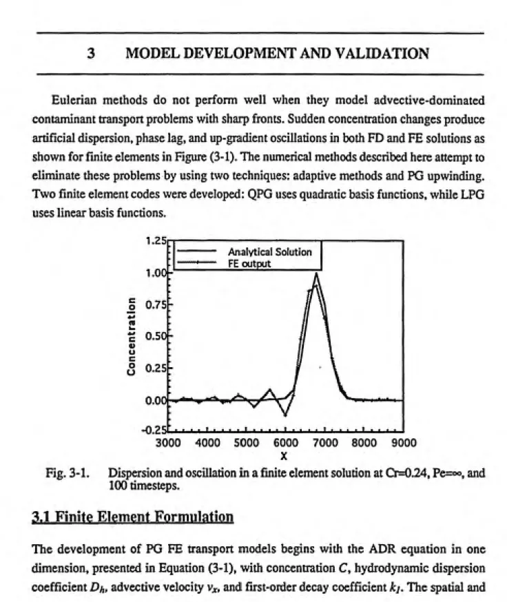
Eulerian methods do not perform well when they model advective-dominated contaminant transport problems with sharp fronts. Sudden concentration changes produce artificial dispersion, phase lag, and up-gradient oscillations in both FD and FE solutions as shown for finite elements in Figure (3-1). The numerical methods described here attempt to
eliminate these problems by using two techniques: adaptive methods and PG upwinding.
Two finite element codes were developed: QPG uses quadratic basis functions, while LPG
uses linear basis functions.
1.25
1.00-g 0.75
^
0.501-u
o 0.25
0.00
-0.251
Analytical Solution
FE output________
,-'—. "ͣ^__z"*^. ^ͣͣp I iftiifti
ͣͣͣ
'•ͣ•ͣ'ͣ •ͣͣ'ͣͣ•
3000 4000 5000 6000 7000 8000 9000
X
Fig. 3-1. Dispersion and oscillation in a finite element solution at Cr=0.24, Pe=oo, and
100 timesteps.
3.1 Finite Element Formulation
temporal dimensions are indicated by x and t, respectively. Linear local equilibrium (LLE) sorption can be easily included by dividing Dh, Vx, and kj by Rf, the retardation factor.
dC ^ d^C dC , _ (3-1)
The following weighted residual expression results from applying weighting functions Wi and integrating over the domain D, which extends from zero to xl with n„ nodes:
f^|t^-{^tc,.4^<,^^
dCjdtdx
(3-2)
= DhWi
dx for/=!,...,n„
Zero-order continuous basis functions are used, so the derivative in the diffusive term is reduced from second- to first-order by Green's theorem. This is a valid operation if the spatial derivative of D/, is small in comparison to the spatial derivative of the concentration, which is generally true for this class of problems. A Dirichlet boundary is located at x=0, and a Neuman boundary makes dC/dx = 0 at x=Xl.
The temporal derivative in Equation (3-2) is then resolved with a Crank-Nicolson finite
difference scheme, to yield:
Di dWi ^ BNj Cj*'^+ Cj
"dx pidx 2
(3-3)
The superscripts / and /+1 indicate the known and unknown time levels, respectively, W^/ is a shorthand notation that represents all n„ weighting functions, and At is the timestep length. Equation (3-3) can be rearranged and expressed in matrix notation as:
[[Aj+i{[AD]+[Av]+[Ak])]{C}'*4[Aj-l{[AD]+[Av]-H[Ak])]{C}' (3-4)
dispersion [Ad], advection [Ay], and first-order decay [Ak]. The sum of [Ap] and [Ay] is
sometimes referred to as the stiffness matrix. These matrices are derived from the portions
of Equation (3-3) that relate to each process, and will be described after the definition of the
basis and weighting functions in the next section.
3.2 Basis and Weighting Functions
Finite element formulations use basis functions to interpolate the dependent variable,
and weighting functions to minimize the difference between the exact and approximated
solutions over each element. The traditional BG FE formulation uses identical basis and
weighting functions, while PG upwinded FE formulations use different weighting and basis
functions. The codes presented here use N+1 and N+2 degree upwinding - the weighting
functions have components that are one and two polynomial orders higher than the basis
functions.
The PG weighting functions used here are composed of the basis functions and
modifying functions that furnish higher-order components. The modifying functions are
multiplied by dimensionless parameters that control the contributions of the N+1 and N+2
degree portions of the upwinding functions. While PG upwinding has been demonstrated to
produce excellent results when applied to sharp-front problems, relatively little information
is available regarding the optimal values of the upwinding parameters a and /3 for transient
ADR models involving sharp fronts.
Linear Lagrange polynomial basis functions {Ni(^)) may be expressed in terms of
natural coordinates (4):
A^ira = ^ (3-5)
A^2{^) = ^ (3-6)
For N+1 and N+2 degree PG upwinding of linear elements, the weighting functions
(Wi(^)) contain quadratic iM2(0) and cubic (M3(^)) modifying functions in addition to the
basis functions.
Wi{x) = Ni(^) - aMi^) - mi^) (3-7)
y^iix) = N2(l) + aW2(l) + mi(^) (3-8)
The dimensionless upwinding parameter a regulates the amount of N+1 degree upwinding,
equivalent to the standard BG formulation. The following quadratic and cubic modifying functions used here were proposed by Dick (1983) and further studied by Westerink and
Shea (1989).
M3(^=|^^l)(^l)
(3-9) (3-10)
-1 -0.5 0 0.5 1 -1 -0.5 0 0.5 1 -1 -0.5 0 0.5
^ 4 ^ Fig. 3-2. (a) Linear basis functions (b) Quadratic modifying function (c) Cubic
modifying function.
(c)
3.
-1 -0.5 0 0.5
0
-1-,mmmm,
^1 ^2
^^^
k^
-H
k
f
1 -0.5 (3 0 5 ] -1 -0.5 0 0.5
I I ^ Fig. 3-3. Weighting functions from linear basis functions and: (a) N+1 degree
The linear basis functions presented in Equations (3-5) and (3-6) are graphed in Figure (3-2(a)) over the range of natural spatial coordinates that span one element. The quadratic modifying function from Equation (3-9) and the cubic modifying function from Equation (3-10) are also graphed in this figure. The resulting weighting functions for various levels of N+1 and N+2 degree upwinding are graphed in Figure (3-3).
Quadratic elements are composed of three quadratic Lagrange polynomial basis
functions - two for the comer nodes at the ends of each element, and one for the mid-element node.
A^i(^) = ^ (3-11)
A^2(d=-^2 + i (3.12)
N3(<D=-^-^ (3-13)
Three weighting functions composed of basis functions and modifying functions are also required. For the upwinding formulation, cubic and quartic modifying functions are used, since second-order basis functions are being upwinded by one and two degrees respectively. Four upwinding parameters are used, Op and j3c for comer nodes and a^ and Pm for mid-element nodes. As for the linear formulation, occ and am affect N+1 upwinding, while j3c and )3ff, control N+2 upwinding.
WiiO = NiiO - cCcM3(0 - )3,M4(a (3-14) W2{^) = N2i^) + 4a„M3{^ + 4Pn,M4i^ (3-15) W3(^ = N2(^-acM3(^-PcMA(x^ (3-16) In the above weighting functions, Mjf^) is the cubic modifying function from Equation (3-10), and M4(^) is the quartic modifying function introduced by Westerink and Shea
(1989).
Af4(^=f^--r+^') (3-17)
m
(a) a.. ͣ---^ 1
J--- ^3 1
9_ 1 _ 0-1 _
^
^s
"""X^
——^*«—.i
1 -0.5 () 0 5 1
(b)
3- -1--1 -0
M,
5 0 0.5
(0
3'
-1
M,
-1 -0.5 0 0.5
4 ^ ^ Fig. 3-4. (a) Quadratic basis functions (b) Cubic modifying function (c) Quartic
modifying function. (b) 3 0 ͣ 1 -1
1 —"^^ 1
1 "^^ 1
1 /
\
/
\
'*—^*—ͣ
\
1 ^\
7^
*N
^
-1 -05 () 0 5 1
-1 -0.5 0 0.5 1 -1 -0.5 0 0.5 1 -1 -0.5 0 0.5
^ \ \
Fig. 3-5. Weighting functions from quadratic basis functions with: (a) N+1 degree
^c=Aw=l-3..^ Coefficient matrices
Coefficient matrices are assembled from the basis and weighting functions by using the differential and integral expressions that appear in Equation (3-3). The coefficient matrices for linear elements can be derived by substituting Equations (3-5) through (3-10) into (3-3) to produce:
[AJ = ^
[Ak] = Axki
1 .a .p.
3 4 24
l.£^+ P.
6 4 24 6 4 24 3 4 24-
l+cc.P.
" 1 .a .P.
3 4 24 6 4 24
-6 4 24 3 4 24
(3-18)
(3-19)
[Av]=|
L-1 -a-1 + a[Ad] =-Dh
Ax
1 -a 1 + a
1 -1
-1 IJ
(3-20)
(3-21)
The intemodal spacing Ax should not be confused with element length. Quadratic elements contain an internal node, so Ax is one half of the element length. The coefficient matrices for quadratic elements in the following equations arise from substituting equations (3-10) through (3-17) into (3-3).
[Aj=f
[Ak] = kiAx
m
4 Oc 3)3c
15 12 40
_2_ Pc
15 5 15 12 40
2 a„ ^Pm
15 3 10
16 , ^Pm
15 5
2 ttn, , 3^m
15 3 10
1 Oc ^Pc
15 12 40
2 Pc,
15 5
4 , OCc ^Pc
15 12 40 J
4 Oc ^Pc
15 12 40
2 Pc
15 5
1 , ac ^Pc
15 12 40
2 1 «« , ^Pm
15 3 10
1^ +
4^-15 5
2 Om /iPm
15 3 ͣ 10
1 Oc ^Pc
15 12 40
2 i3.
15 5
4 , ttc 3^c
15 12 40
(3-22)
[Av] = 2v, i ͣ 4 1 3 X L 12
12 80
3
^n^
20
80
[Ad] =_2Dh
Ax
12 40
2 ZA«
3
1
10 112"^ 40
i ^ 3 ' 6
3
3 6 2. Z^ 3 20
3 5
2 Z& 3 20
i.
3
12 80
3 20
12 80
1 ."^^^l
12 402 7)8«
3 10
7 ,7^c
12 40J
27
(3-24)
(3-25)
3.4 Adaptive Method
The adaptive method used in this work is derived from a 1-D h-meihod proposed by G.T. Yeh (1988). The advantage in this approach lies in that the additional nodes produced by mesh refinement are placed in matrices that are isolated from the unrefined global matrix. This results in code that is less complex than what would result from renumbering and reassembling the global matrices, as fewer operations are required, and less computer memory is needed. Soon after its introduction, this method was extended to 2-D in the form of an Eulerian-Lagrangian hybrid in which advection is modeled with the Lagrangian single-step reverse particle tracking method, and the other processes in the problem are
handled with an Eulerian (FE) method (Yeh, 1990).
In the 1-D method, spatial elements are uniformly subdivided into smaller subelements for the solution at the next timepoint if a sharp front is detected within the element at the current solution level. Other elements may also be subdivided, depending on user-definable parameters that allow mesh refinement to be projected along the advective path, permitting refinement of elements that are expected to contain the front at the next solution level. The degree of refinement is also user-defined. The LPG code can subdivide elements by any positive number, while QPG is restricted to even positive numbers of subelements by constraints imposed by the adaptive algorithm.
adjusted and solved. This method results in solutions that are exactly the same as if all nodes had been represented by a single matrix.
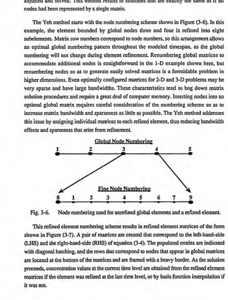
The Yeh method starts with the node numbering scheme shown in Figure (3-6). In this example, the element bounded by global nodes three and four is refined into eight subelements. Matrix row numbers correspond to node numbers, so this arrangement allows an optimal global numbering pattern throughout the modeled timespan, as the global numbering will not change during element refinement. Renumbering global matrices to accommodate additional nodes is straightforward in the 1-D example shown here, but renumbering nodes so as to generate easily solved matrices is a formidable problem in
higher dimensions. Even optimally configured matrices for 2-D and 3-D problems may be
very sparse and have large bandwidths. These characteristics tend to bog down matrix solution procedures and require a great deal of computer memory. Inserting nodes into an optimal global matrix requires careful consideration of the numbering scheme so as to increase matrix bandwidth and sparseness as little as possible. The Yeh method addresses
this issue by assigning individual matrices to each refined element, thus reducing bandwidth
effects and sparseness that arise from refinement
Global Node Numbering
2 3 4
Fine Node Numhering
2 3 4 5 6
Fig. 3-6. Node numbering used for unrefined global elements and a refined element
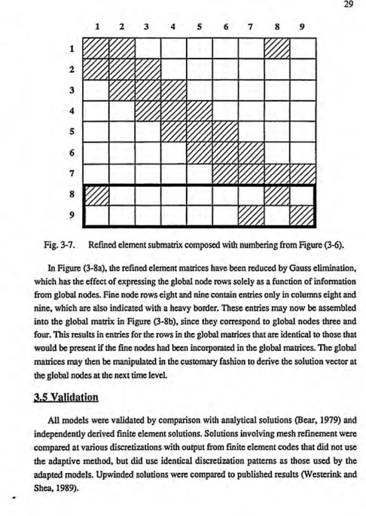
This refined element numbering scheme results in refined element matrices of the form shown in Figure (3-7). A pair of matrices are created that correspond to the left-hand-side
(LHS) and the right-hand-side (RHS) of equation (3-4). The populated entries are indicated with diagonal hatching, and the rows that correspond to nodes that appear in global matrices
are located at the bottom of the matrices and are fi-amed with a heavy border. As the solution
proceeds, concentration values at the current time level are obtained fiiom the refined element matrices if the element was refined at the last time level, or by basis function interpolation if