Rare variant association testing for sequencing data.pdf

(1)

ARTICLE

Rare-Variant Association Testing

for Sequencing Data with the Sequence

Kernel Association Test

Michael C. Wu,

1,5

_{Seunggeun Lee,}

2,5

_{Tianxi Cai,}

2

_{Yun Li,}

1,3

_{Michael Boehnke,}

4

_{and Xihong Lin}

2,

_*

Sequencing studies are increasingly being conducted to identify rare variants associated with complex traits. The limited power of clas-sical single-marker association analysis for rare variants poses a central challenge in such studies. We propose the sequence kernel asso-ciation test (SKAT), a supervised, flexible, computationally efficient regression method to test for assoasso-ciation between genetic variants (common and rare) in a region and a continuous or dichotomous trait while easily adjusting for covariates. As a score-based vari-ance-component test, SKAT can quickly calculate p values analytically by fitting the null model containing only the covariates, and so can easily be applied to genome-wide data. Using SKAT to analyze a genome-wide sequencing study of 1000 individuals, by segment-ing the whole genome into 30 kb regions, requires only 7 hr on a laptop. Through analysis of simulated data across a wide range of practical scenarios and triglyceride data from the Dallas Heart Study, we show that SKAT can substantially outperform several alternative rare-variant association tests. We also provide analytic power and sample-size calculations to help design candidate-gene, whole-exome, and whole-genome sequence association studies.

Introduction

Genome-wide association studies (GWASs) have identified

more than 1000 genetic loci associated with many human

diseases and traits,

1

yet common variants identified

through GWASs often explain only a small proportion of

trait heritability. The advent of massively parallel

sequencing

2

has transformed human genetics

3,4

and has

the potential to explain some of this missing heritability

through identification of trait-associated rare variants.

5

Although considerable resources have been devoted to

sequence mapping and genotype calling,

6–9

_successful

application of sequencing to the study of complex traits

requires novel statistical methods that allow researchers

to test efficiently for association given data on rare

vari-ants

10

and to perform sample-size and power calculations

to help design sequencing-based association studies.

Rare genetic variants, here defined as alleles with

a frequency less than 1%–5%, can play key roles in

influ-encing complex disease and traits.

11

However, standard

methods used to test for association with single common

genetic variants are underpowered for rare variants unless

sample sizes or effect sizes are very large.

12,13

A logical

alter-native approach is to employ burden tests that assess

the cumulative effects of multiple variants in a genomic

region.

12–18

_{Burden tests proposed to date are based on}

collapsing or summarizing the rare variants within a region

by a single value, which is then tested for association with

the trait of interest. For example, the cohort allelic sum test

(CAST)

14

_{collapses information on all rare variants within}

a region (e.g., the exons of a gene) into a single

dichoto-mous variable for each subject by indicating whether or

not the subject has any rare variants within the region

and then applies a univariate test. Instead of collapsing by

dichotomizing the number of rare variants within a region,

collapsing by counting them is also possible.

18

The

combined multivariate and collapsing method

12

extends

CAST by collapsing rare variants within a region into

subgroups on the basis of allele frequency, collapsing

subgroups as in CAST, and applying a multivariate test to

the subgroups. The weighted sum test (WST)

13

specifically

considers the case-control setting and collapses a set of

SNPs into a single weighted average of the number of

rare alleles for each individual. Numerous alternative

methods are largely variations on these approaches.

16,17,19

A limitation for all these burden tests is that they

implic-itly assume that all rare variants influence the phenotype

in the same direction and with the same magnitude of

effect (after incorporating known weights). However, one

would expect most variants (common or rare) within

a sequenced region to have little or no effect on

pheno-type, whereas some variants are protective and others

dele-terious, and the magnitude of each variant’s effect is likely

to vary (e.g., rarer variants might have larger effects).

Hence, collapsing across all variants is likely to introduce

substantial noise into the aggregated index, attenuate

evidence for association, and result in power loss.

Further-more, burden tests require either specification of

thresh-olds for collapsing or the use of permutation to estimate

the threshold.

16–20

_{Permutation tests are computationally}

expensive, especially on the whole-genome scale, and are

difficult for covariate adjustment because permutation

1_{Department of Biostatistics, The University of North Carolina at Chapel Hill, Chapel Hill, NC 27599, USA;}2_{Department of Biostatistics, Harvard School} of Public Health, Boston, MA 02115, USA;3_{Department of Genetics, The University of North Carolina at Chapel Hill, Chapel Hill, NC 27599, USA;}4 Depart-ment of Biostatistics and Center for Statistical Genetics, University of Michigan, Ann Arbor, MI 48109, USA

5_{These authors contributed equally to this work}

*Correspondence:[email protected]

(2)

requires independence between the genotype and the

co-variates.

The recently proposed C-alpha test

21

is a

non-burden-based test and is hence robust to the direction and

magni-tude of effect. For case-control data, it compares the

expected variance to the actual variance of the distribution

of allele frequencies. These important advantages allow the

C-alpha test to have improved power over burden-based

tests, especially when the effects are in different directions.

Despite these attractive features, the C-alpha test does not

allow for easy covariate adjustment, such as for controlling

population stratification, which is important in genetic

association studies. The C-alpha test also uses permutation

to obtain a p value when linkage disequilibrium is present

among the variants, which is, as noted earlier,

computa-tionally expensive for whole-genome experiments. The

approach has not been generalized to analysis of

contin-uous phenotypes.

We propose in this paper the sequence kernel association

test (SKAT), a flexible, computationally efficient, regression

approach that tests for association between variants in a

region (both common and rare) and a dichotomous (e.g.,

case-control) or continuous phenotype while adjusting for

covariates, such as principal components, to account for

population stratification.

22

The kernel machine regression

framework was previously considered for common

vari-ants.

23,24

In this paper, we provide several essential

method-ological improvements necessary for testing rare variants.

SKAT uses a multiple regression model to directly regress

the phenotype on genetic variants in a region and on

cova-riates, and so allows different variants to have different

directions and magnitude of effects, including no effects;

SKAT also avoids selection of thresholds. We develop a

kernel association test to test the regression coefficients of

the variants by using a variance-component score test in a

mixed-model framework by accounting for rare variants.

SKAT is computationally efficient. This quality is

espe-cially important in genome-wide studies because SKAT

only requires fitting the null model in which phenotypes

are regressed on the covariates alone; p values are easily

computed with simple analytic formulae. Additional

features of SKAT include exploitation of local correlation

structure, incorporation of flexible weights to boost power

(e.g., by increasing the weight of rarer variants or

incorpo-rating functionality), and allowance for epistatic variant

effects. As discussed in more detail below, under special

cases, the SKAT, C-alpha test, and individual variant test

statistics are closely related.

We demonstrate through simulation and analysis of

resequencing data from the Dallas Heart Study that SKAT

is often more powerful than existing tests across a broad

range of models for both continuous and dichotomous

data. We also investigate the factors that influence power

for sequence association studies. Finally, we describe

analytic tools to estimate statistical power and sample sizes

to guide the design of new sequence association studies of

rare variants with SKAT.

Material and Methods

Sequencing Kernel Association Test

SKAT is a supervised test for the joint effects of multiple variants in a region on a phenotype. Regions can be defined by genes (in candidate-gene or whole-exome studies) or moving windows across the genome (in whole-genome studies). For each region, SKAT analytically calculates a p value for association while adjust-ing for covariates. Adjustments for multiple comparisons are necessary for analyzing multiple regions, for example with the Bonferroni correction or FDR control.

Notation

Assumensubjects are sequenced in a region withpvariant sites observed. Covariates might include age, gender, and top principal components of genetic variation for controlling population strat-ification.22For thei-th subject,yidenotes the phenotype variable,

Xi¼(Xi1, Xi2, .., Xim) denotes the covariates, andGi¼(Gi1, Gi2,., Gip) denotes the genotypes for thepvariants within the region. Typically, we assume an additive genetic model and letGij,¼0, 1, or 2 represent the number of copies of the minor allele. Domi-nant and recessive models can also be considered.

SKAT Model and Test for Linear SNP Effects

For a simple illustration of SKAT, we focus here on testing for a rela-tionship between the variants and the phenotype by using clas-sical multiple linear and logistic regression. We describe how the SKAT can incorporate epistatic effects later. To relate the sequence variants in a region to the phenotype, consider the linear model

yi¼a0þa0Xiþb0Giþ3i; (Equation 1) when the phenotypes are continuous traits, and the logistic model

logitPyi¼1

¼a0þa0Xiþb0Gi; (Equation 2)

when the phenotypes are dichotomous (e.g.,y¼0/1for case or control). Herea0is an intercept term,a¼[a1,.,am]’ is the vector of regression coefficients for themcovariates,b¼[b1,.,bp]’ is the vector of regression coefficients for thepobserved gene variants in the region, and for continuous phenotypes3iis an error term with a mean of zero and a variance ofs2. Under both linear and logistic models, and evaluating whether the gene variants influence the phenotype, adjusting for covariates, corresponds to testing the null hypothesis H0:b¼0, that is,b1¼b2¼.¼bp¼0. The stan-dard p-DF likelihood ratio test has little power, especially for rare variants. To increase the power, SKAT tests H0by assuming each

bj follows an arbitrary distribution with a mean of zero and a variance ofwjt, wheretis a variance component andwjis a pre-specified weight for variantj. One can easily see that H0:b¼0is

equivalent to testing H0:t¼0, which can be conveniently tested

with a variance-component score test in the corresponding mixed model; this is known to be a locally most powerful test.25A key advantage of the score test is that it only requires fitting the null model yi¼a0 þa1’Xiþ3ifor continuous traits and the logit P(yi¼1)¼a0þa1’Xifor dichotomous traits.

Specifically, the variance-component score statistic is

Q¼ybm0Kymb; (Equation 3) whereK¼GWG’,mbis the predicted mean ofyunder H0, that is

b

m¼ba0þXba for continuous traits andmb¼logit1ðba0þXbaÞfor

dichotomous traits; and ba0andabare estimated under the null

model by regressing y on only the covariatesX. HereGis an

(3)

variantjof subjecti, andW¼diag(w1,., wp) contains the weights of thepvariants.

In fact,Kis ann₃nmatrix with the (i, i’)-th element equal to

KðGi;Gi0Þ ¼Pp_j_¼₁wjGijGi0j.Kð,;,Þis called the kernel function, and

K_ðGi;Gi0Þmeasures the genetic similarity between subjectsiandi’ in the region via thepmarkers. This particular form ofKð,;,Þis called the weighted linear kernel function. We later discuss other choices of the kernel to model epistatic effects.

Good choices of weights can improve power. Each weightwj is prespecified, with only the genotypes, covariates and external biological information, that is estimated without using the outcome, and reflects the relative contribution of thej-th variant to the score statistic: ifwj is close to zero, then thej-th variant makes only a small contribution to Q. Thus, decreasing the weight of noncausal variants and increasing the weight of causal variants can yield improved power. Because in practice we do not know which variants are causal, we propose to set

ffiffiffiffiffi

wj

p ¼Beta_ðMAFj;a1;a2Þ, the beta distribution density function

with prespecified parametersa1anda2evaluated at the sample

minor-allele frequency (MAF) (across cases and controls combined) for thej-th variant in the data. The beta density is flex-ible and can accommodate a broad range of scenarios. For example, if rarer variants are expected to be more likely to have larger effects, then setting 0 < a1 %1 and a2 R1 allows for increasing the weight of rarer variants and decreasing the weight of common weights. We suggest settinga1¼1 anda2¼25 because it increases the weight of rare variants while still putting decent nonzero weights for variants with MAF 1%–5%. All simulations were conducted with this default choice unless stated otherwise. Note that a smaller a1 results in more strongly increasing the weight of rarer variants. Examples of weights across a range ofa1anda2values are presented inFigure S1, available online. Note thata1¼a2¼1 corresponds towj¼1, that is all variants are weighted equally, and a1 ¼ a2 ¼ 0.5 corresponds to

ffiffiffiffiffi

wj

p ¼1=pffiffiffiffiffiffiffiffiffiffiffiffiffiffiffiffiffiffiffiffiffiffiffiffiffiffiffiffiffiffiffiffiffiffiffiMAFjð1MAFjÞ, that iswjis the inverse of the variance of the genotype of markerj, which puts almost zero weight for MAFs>1% and can be used if one believes only variants with MAF< 1% are likely to be causal. Note that SKAT calculated with this weight is identical to the unweighted SKAT test with the standardized genotypes inEquations 1 and 2. Other forms of the weight as a function of MAF can also be used. Because SKAT is a score test, the type I error is protected for any choice of pre-chosen weights. Note that the weights used in the weighted sum test13 involve phenotype information and will therefore alter the null distribution of SKAT if such weights are used.

Under the null hypothesis,Qfollows a mixture of chi-square distributions, which can be closely approximated with the compu-tationally efficient Davies method.26_See_{Appendix A}_{for details.}

A special case of SKAT arises when the outcome is dichotomous, no covariates are included, and allwj¼1. Under these conditions, we show inAppendix Athat the SKAT test statisticQis equivalent to the C-alpha test statisticT. Hence, the C-alpha test can be seen as a special case of SKAT, or alternatively, SKAT can be seen as a generalized C-alpha test that does not require permutation but calculates the p value analytically, allows for covariate adjust-ment, and accommodates either dichotomous or continuous phenotypes. Because SKAT under flat weights is also equivalent to the kernel machine regression test23,24_{and because the kernel}

machine regression test is in turn related to the SSU test,27 it follows transitively that SKAT under flat weights, the kernel machine regression test, the SSU test, and the C-alpha test are all equivalent and special cases of SKAT. Note that the null

distribu-tion is calculated differently via these methods, and SKAT gives more accurate analytic p values, especially in the extreme tail, when sample sizes are sufficient.

Relationship between Linear SKAT and Individual Variant Test Statistics

One can efficiently compute the test statistic Q by exploiting a close connection between the SKAT score test statisticQand the individual variant test statistics. In particular,Qis a weighted sum of the individual score statistics for testing for individual variant effects. Hence, by letting gj ¼[G1j,G1j,., Gnj]’ denote then31 vector containing the genotypes of thensubjects for variant j, it is straightforward to see thatQ_¼Pp_j_¼₁wjS2j, where

Sj¼g0jðybm0Þ is the individual score statistic for testing the

marginal effect of thej-th marker (H0:bj¼0) under the individual linear or logistic regression model ofyionXiand only the j-th variantGij:

yi¼a0þX0iaþbjGijþ3i for continuous phenotypes and

logitPyi¼1

¼a0þX0iaþbjGij

for dichotomous phenotypes.mb0 is estimated asbm0¼ba0þX0iba

for continuous traits andbm0¼logit 1

ðba0þX0ibaÞfor dichotomous

traits. As a score test, one needs to fit the null model only a single time to be able to compute theSjfor all individual variantsjas well as all regions to be tested. Similarly, if multiple regions are under consideration, then the same bm0 can be used to compute the

SKATQstatistics for each region.

Accommodating Epistatic Effects and Prior Information under the SKAT

An attractive feature of SKAT is the ability to model the epistatic effects of sequence variants on the phenotype within the flexible kernel machine regression framework.28–30_{To do so, we replace} Gi’bby a more flexible functionf(Gi) in the linear and logistic models (1) and (2) where f(Gi) allows for rare variant by rare variant and common variant by rare-variant interactions. Specifi-cally, for continuous traits we use the semiparametric linear model23,29

yi¼a0þa0XiþfðGiÞ þ3i; (Equation 4)

and for dichotomous traits, we use the semiparametric logistic model24,30

logitPyi¼1

¼a0þa0XiþfðGiÞ: (Equation 5)

Here the variants,Gi, are related to the phenotype through a possibly nonparametric functionf($), which is assumed to lie in a functional space generated by a positive semidefinite kernel functionK_ð_,_;_,_Þ. Models (1) and (2) assume linear genetic effects and are specified by KðGi;Gi0Þ ¼P_jp_¼₁wjGijGi0j. By changing

K_ð_,_;_,_Þ, one can allow for more complex models. Intuitively,

KðGi;Gi0Þis a function that measures genetic similarity between thei-th andi’-th subjects via thepvariants in the region, and any positive semidefinite function KðGi;Gi0Þ can be used as a kernel function. We tailored several useful and commonly used kernels specifically for the purpose of rare-variant analysis: the weighted linear kernel, the weighted quadratic kernel, and the weighted identity by state (IBS) kernel.

The weighted linear kernel function KðGi;Gi0Þ ¼Pp_j_¼₁wjGijGi0j

implies that the trait depends on the variants in a linear fashion and is equivalent to the classical linear and logistic model pre-sented in Equations 1 and 2. The weighted quadratic kernel

KðGi;Gi0Þ ¼ ð1þPjp¼1wjGijGi0jÞ2implicitly assumes that the model

(4)

variants and the first-order variant by variant interactions. The weighted IBS kernelK_ðGi;Gi0Þ ¼Pp_j_¼₁wjIBSðGij;Gi0jÞ, defines

simi-larity between individuals as the number of alleles that share IBS. For additively coded autosomal genotype data,K_ðGi;Gi0Þ ¼ Pp

j¼1wjð2 jGijGi0jjÞ. The model implied by the weighted IBS

kernel models the SNP effects nonparametrically.31_{Consequently,}

this allows for epistatic effects because the functionf($) does not assume linearity or interactions of a particular order (e.g., the second order), Using the weighted IBS kernel removes the assump-tion of additivity because the number of alleles that are identical by state is a physical quantity that does not change on the basis of different genotype encodings.

We note that a kernel function that better captures both the similarity between individuals and the causal variant effects will increase power. In particular, if relationships are linear and no interactions are present, then the weighted linear kernel will have highest power. If interactions are present, the weighted quadratic and weighted IBS kernels can increase power. Our expe-rience suggests using the IBS kernel when the number of interact-ing variants within the region is modest. As our understandinteract-ing of genetic architecture improves so too will our knowledge of which kernel to use.

In each of the above kernels,wjis an allele specific weight that controls the relative importance of thejthvariant and might be a function of factors such as allele frequency or anticipated func-tionality. Without prior information, we suggest the use of the

ffiffiffiffiffi

wj

p ¼Beta_ðMAFj;1;25Þsuggested earlier. However, if prior

infor-mation is available, for example some variants are predicted as functional or damaging via Polyphen32_{or Sift,}33_{weights can be}

selected to increase the weight for likely functionality.

To test for the effects of gene variants in a region on a phenotype, one tests the null hypothesis H0:f(G)¼0. SKAT tests for this null

hypothesis by assuming then31 vectorf¼[f(G1),.,f(Gn)]’ for the genetic effects ofnsubjects follows a distribution with mean zero and covariancetK,where t is a variance component that indexes the effects of the variants.29,30_{Hence, we can test the}

null hypothesis that corresponds to testing H0: t¼0 by a

vari-ance-component score test. In particular, we simply replaceKin

Equation 3by using theKdiscussed in this section, for example, the weighted IBS kernel, for epistatic effect. All subsequent calcu-lations for computing a p value remain the same.

Because the SKAT evaluates significance via a score test, which operates under the null hypothesis, the SKAT is valid (in terms of protecting type I error) irrespective of the kernel and the weights used. Good choices of the kernel and the weights simply increase power.

Planning New Sequencing-Based Association Studies:

Estimation of Power and Sample Size

Power and sample-size calculations are important in designing sequencing studies of complex traits. Using a modification of the higher-order moment-approximation method,34we provide an analytic method to carry out efficiently such calculations for SKAT.35Specifically, for a fixed sample size andalevel, given a prior hypothesis on the genetic architecture of a particular region, the effect size, and the proportion and number of causal variants within a region, our method provides the power to detect the region as significant with SKAT. Similarly, if the desired power is fixed, the approach can be used to find the necessary sample size. There are key differences between the power and sample-size estimation for single-variant- and region (set)-based tests. For a region (set)-based test, the power depends strongly on the

under-lying genetic architecture, and its estimation requires modeling this genetic architecture and the linkage disequilibrium (LD) between variants. Therefore, to estimate power to detect a partic-ular region as associated with a phenotype requires specification of the significance level, sample size, which variants in the region are causal with corresponding effect size, and the LD structure of the variants in the region. Ideally, one could use prior data to assess the LD and MAF. Because prior data can be difficult to obtain, we currently recommend the use of either 1000 Genomes Project data36 or data simulated under a population genetics model.37 _{Relevant preliminary data will become increasingly}

available as sequencing studies become more common.

Our SKAT software uses simulated data based on the coalescent population genetic model (released with the software package) as a default in performing sample-size and power calculations, and instead of directly specifying the effects of any given variant, the user can input an MAF threshold for determining which variants are regarded as rare and also a proportion determining how many of the rare variants are causal. The causal variants are then randomly selected from the alleles with true MAF (based on simulated or preliminary data) less than the threshold. The magnitudes of the effectsjbjjfor causal variants are set to be equal toc3jlog10MAFj

wherecis determined on the basis of the maximum effect size the user would like to allow (described below in the power simulations section) at MAF¼104_{. This allows the effects of causal variants to}

decrease with MAFs. Because these parameters can be difficult to choose as a priori, power and sample size can be reasonably estimated by averaging results over a range of parameter values. Similarly, because the regional architecture can vary across different regions, for genome-wide studies, one can average over multiple randomly selected regions as currently implemented in the SKAT software.

Numerical Experiments and Simulations

To validate SKAT in terms of protecting type I error and to assess its power compared to burden tests and the accuracy of our power and sample-size tools, we carried out simulation studies under a range of configurations. For all simulations, we determined sequence genotypes by simulating 10,000 chromosomes for a 1 Mb region on the basis of a coalescent model that mimics the LD pattern local recombination rate and the population history for Europeans by using COSI.37

Type I Error Simulations

To investigate whether SKAT preserves the desired type I error rate at the near genome-wide threshold level, for examplea¼106, it is necessary to conduct simulations with hundreds of millions of simulated datasets. Although SKAT is computationally efficient, generating such a large number of datasets is challenging. To reduce the computation burden, we took the following approach. Using 10,000 randomly selected sets of 30 kb subregions within a 1 Mb chromosome, we first generated 10,000 sets of genotypes

G(n3p)from the coalescent model, withpvariants onnsubjects. Then, for each of the 10,000 simulated genotype data sets, we simulated 10,000 sets of continuous phenotypes such that we were able to obtain 108_{individual genotype-phenotype data sets}

by using the model:

y¼0:5X1þ0:5X2þ3;

(5)

which the genotype values are based contained 605 variants on average, but the number of observed variants for any given data set was considerably less and depended on the sample sizen, which we set to 500, 1000, 2500, and 5000.

We repeated the type I error simulations for dichotomous phenotypes as above, except the dichotomous outcomes were generated via the model:

logitP_ðy_¼1Þ ¼a0;

wherea0was determined to set the prevalence to 1% and

case-control sampling is used.

For both continuous and dichotomous simulations, we applied SKAT by using the default weighted linear kernel to each of the 108 data sets and estimated the empirical type I error rate as the proportion of p values less thana¼104, 105, or 106.

We note that the estimated type I error from this approach is not the same as the empirical type I error when genotypes are generated randomly for each simulation, because for each of the

10,000 genotype data sets, only the outcomes are resampled. However, our type I error estimator is still unbiased and results in very accurate type I error estimates. For largeralevels (0.05 and 0.01), we directly computed the empirical type I error rate by using data sets in which genotypes were randomly generated for each simulation.

Empirical Power Simulations

We simulated data sets in which 30 kb subregions were randomly selected from the generated 1 Mb chromosomes and used to create causal variants and a phenotype variable as well as additional simulated covariates. We generated continuous phenotypes by

y¼0:5X1þ0:5X2þb1Gc1þb2Gc2þ.þbpGcpþ3;

whereX1,X2, and3are as defined for the type I error simulations, Gc

1;Gc2;.;Gcs are the genotypes of the s causal rare variants (a

randomly selected subset of the simulated rare variants, for example 5% of variants that have MAF< 3% inFigure 1), and the bs are effect sizes for the causal variants. Similarly, we

0.5k 1k 2.5k 5k

0.0

0.2

0.4

0

.6

0.8

1

.0 β +/− = 100/0

Total Sample Size

Po

w

e

r

SKAT SKAT_M rSKAT W N C

0.5k 1k 2.5k 5k

0.0

0.2

0.4

0

.6

0.8

1

.0 β +/− = 80/20

Total Sample Size

Po

w

e

r

0.5k 1k 2.5k 5k

0.0

0.2

0.4

0

.6

0.8

1

.0 β +/− = 50/50

Total Sample Size

Po

w

e

r

Continuous Trait

0.5k 1k 2.5k 5k

0.0

0.2

0.4

0

.6

0.8

1

.0 β

+/− = 100/0

Total Sample Size

Po

w

e

r

0.5k 1k 2.5k 5k

0.0

0.2

0.4

0

.6

0.8

1

.0 β

+/− = 80/20

Total Sample Size

Po

w

e

r

0.5k 1k 2.5k 5k

0.0

0.2

0.4

0

.6

0.8

1

.0 β

+/− = 50/50

Total Sample Size

Po

w

e

r

Dichotomous Trait

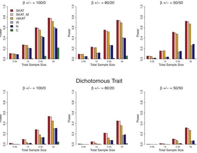
Figure 1. Simulation-Study-Based Power Comparisons of SKAT and Burden Tests

Empirical power ata¼106under an assumption that 5% of the rare variants with MAF<3% within random 30 kb regions were causal. Top panel: continuous phenotypes with maximum effect size (jbj) equal to 1.6 when MAF¼104_{; bottom panel: case-control studies}

with maximum OR¼5 when MAF¼104_{. Regression coefficients for the}_s_{causal variants were assumed to be a decreasing function}

of MAF asjbjj ¼cjlog10MAFjj(j¼1,.,p[seeFigure S2]), wherecwas chosen to result in these maximum effect sizes. From left to right,

(6)

generated dichotomous phenotypes for case-control data under the logistic model

logitP_ðy_¼1Þ ¼a0þ0:5X1þ0:5X2þb1G

c

1þb2G

c

2þ.þbpG c p;

whereGc

1;Gc2;.;Gcp are again the genotypes for the causal rare

variants andbs are log ORs for the causal variants. We controlled prevalence bya0and set to it 1% unless otherwise stated. Under both models, we set the magnitude of eachbj to cjlog10MAFjj

such that rarer variants had larger effects. In the simulation studies, for continuous traits,c¼0.4, which gives the maximum effect sizejbjj ¼1.6 for variants with MAF¼104and small effects

jbjj ¼0.28 for MAF¼ 0.2. For dichotomous traits,c¼ln5/4¼ 0.402, which gives the ‘‘maximum’’ OR¼5.0 (jbjj ¼ln5) for vari-ants with MAF¼104and smaller OR¼1.32 for MAF¼0.2. The effect size curves are given inFigure S2.

We compared SKAT, an unsupervised variation on the WST13

that uses weighted-count-based collapsing, counting-based collapsing,18_{and CAST.}14_{For each of these tests, we considered}

variants with observed MAF<3% as rare: whether CAST collapses depends on whether an individual exhibits any variants with allele frequency<3%, the counting method counts the number variants with MAF< 3%, and the weighted count inflates the contribution of each rare variant by multiplying the genotype with the same beta-density-based weights as used in SKAT.

To accommodate missing genotypes commonly observed in sequence data, we considered the effect of imputing missing values by randomly setting 10% of the genotypes as missing, imputing genotypes on the basis of observed allele frequencies and Hardy-Weinberg equilibrium, and then applying SKAT to the imputed data. We also performed restricted SKAT (rSKAT) by applying unweighted SKAT to rare variants with MAF < 3%. Note that for dichotomous phenotypes, rSKAT is essentially equiv-alent to a covariate adjusted C-alpha test with the p value calcu-lated analytically instead of via permutation. For each of the methods, power was estimated as the proportion of p values<a, wherea¼106_{to mimic genome-wide studies.}

Power and Sample-Size Formulae

To demonstrate the utility and accuracy of our power and sample-size calculation method, we conducted several numerical experi-ments. We first illustrated the use of the methods by computing the sample size necessary to detect a 30 kb region with 5% of the variants with MAF<3% being causal. We assume effect size (OR) increases with decreasing MAF, and seek 80% power at significance levelsa¼106, 103, 102, corresponding to approx-imate genome-wide sequencing significance and candidate-gene-sequencing studies of 50 and five genes, respectively. We consid-ered both continuous and dichotomous traits.

To show that the power estimated from our sample-size formula is accurate, we compared empirical power for SKAT under simula-tions to power estimated via our analytic method. Specifically, we simulated continuous and case-control data under the same setting as that used in the power simulations, and we estimated power as a function of the sample size by computing the propor-tion of p values<a¼106and compared the empirical power curve to the power estimated by using our analytical method.

Results

Simulation of the Type I Error

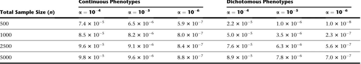
The empirical type I error rates estimated for SKAT are

pre-sented in

Table 1

for

a

¼

10

4

_{, 10}

5

_{, and 10}

6

_{and suggest}

the type I error rate is protected for continuous

pheno-types, though for smaller sample sizes the SKAT can be

slightly conservative. For dichotomous phenotypes, SKAT

is conservative for smaller sample sizes and very small

a

levels. Additional results from simulations of the type I

error for SKAT and the competing methods are presented

in

Figure S3

for both continuous traits and dichotomous

traits and show that at larger

a

levels, all of the considered

tests correctly control at the

a

¼

0.05 and 0.01 levels. These

results show that SKAT is a valid method, and despite being

conservative at low

a

levels, SKAT maintains good power

relative to existing methods (see below). However, if

sample sizes are small or sharp control of type I error is

necessary, then standard permutation-based procedures

can be used to generate a Monte Carlo p value for

signifi-cance, though this can be computationally expensive

and does not work in the presence of covariates, such as

controlling for population stratification and require carful

modifications.

Statistical Power of SKAT and Competing Methods

We compared the power of SKAT with three burden tests

in a series of simulation studies for both continuous traits

and dichotomous traits by generating sequence data

in randomly selected 30 kb regions with a coalescent

model.

37

_{For our primary power simulation, within each}

region, 5% of variants with population MAF

<

3% were

randomly chosen as causal, the effect size of causal variants

was a decreasing function of MAF, and 50%–100% of the

causal variants being positively associated with the trait

Table 1. Type I Error Estimates of SKAT Aimed at Testing an Association between Randomly Selected 30 kb Regions with a Continuous Trait at Type I Error Rates as Low as the Genome-widea¼106_Level

Total Sample Size (n)

Continuous Phenotypes Dichotomous Phenotypes

a¼104 _a_¼₁₀5 _a_¼₁₀6 _a_¼₁₀4 _a_¼₁₀5 _a_¼₁₀6

(7)

(See

Materials and Methods

and

Figure S2

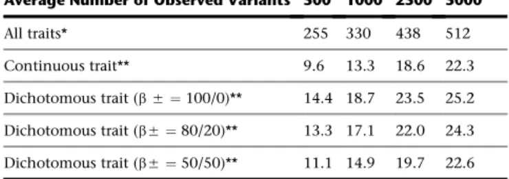
). The simulated

regions for our power analysis contained on average

605 variants (26 causal), of which 530.9 (88%), 502.9

(83%), and 422.8 (70%) had population MAF

<

3%,

<

1%,

and

<

0.1%, respectively. The average allele frequency

spec-trum across the samples is similar to that of the Dallas Heart

Study data (

Figure S4

). Because the majority of variants have

a low MAF, they might not be observed in any particular

sample. The average number of observed variants

(assuming no genotyping error) and the average number

of observed causal variants are presented in

Table 2

.

For continuous traits, SKAT had much higher power

than all the burden tests, and the weighted count method

tended to outperform the count and CAST methods

(

Figure 1

). SKAT’s power was robust to the proportion of

causal variants that were positively associated with the

trait, whereas the burden tests suffered substantial loss of

power when causal variants had the opposite effects. The

simulation results examining dichotomous traits were

qualitatively similar in that SKAT dominated the

compet-ing methods. However, here the power of the SKAT

decreased when both protective and harmful variants

were present, although less so than for the burden tests.

The difference in power for SKAT for different proportions

of protective variants is due to the fact that given fixed

population MAFs, protective variants imply negative log

ORs and lower disease risk and hence lower MAFs in cases

and more difficulties in observing rare variants in cases.

The larger decrease in power for the competing methods

is additionally driven by sensitivity to direction of effect

due to aggregation of genotypes. Across all configurations,

using imputed genotypes instead of the true genotype

for 10% missing genotype data led to a very small

reduction in power, despite the use of a very simple

Hardy-Weinberg-based imputation strategy. This is true

in part because most variants are rare.

Note that SKAT increases the weight of rare variants but

does not require thresholding. To show that the superior

performance of SKAT is intrinsic and is not driven by the

particular choice of the weight used, we calculated rSKAT,

which does not weight the rare variants but instead uses

the same threshold as the burden tests. Our results,

pre-sented in

Figure 1

, show that rSKAT is still substantially

more powerful than all three burden tests.

Power simulation results for other type I error rates (

a

¼

0.01, 0.001), lower causal variant frequencies (population

MAF

<

1%), and other region sizes (10 kb and 60 kb)

yielded the same conclusions (

Figures S5–S8

).

In the 30 kb genomic regions considered, reflecting

anal-ysis of genome-wide sequencing data, it is unlikely that

a large proportion of the rare variants are all causal.

However, for exome-scale sequencing, the number of

observed rare variants can be considerably smaller and

the proportion of causal rare variants can be greater.

Hence, we also conducted power simulations for smaller

region sizes (3 kb and 5 kb) and larger proportions of causal

variants (10%, 20%, and 50%). Results for both continuous

and dichotomous phenotypes are presented in

Figures S9–

S12

and show that if 50% of the rare variants are causal and

that all of the causal variants have effects in the same

direc-tion, then SKAT and rSKAT are less powerful compared to

collapsing methods, with count-based collapsing having

the greatest power. This result held for both 3 kb and

5 kb regions and is expected because the collapsing

methods implicitly assume that all of the variants are

causal and have unidirectional effects. In all other settings

we considered, SKAT was the most powerful method.

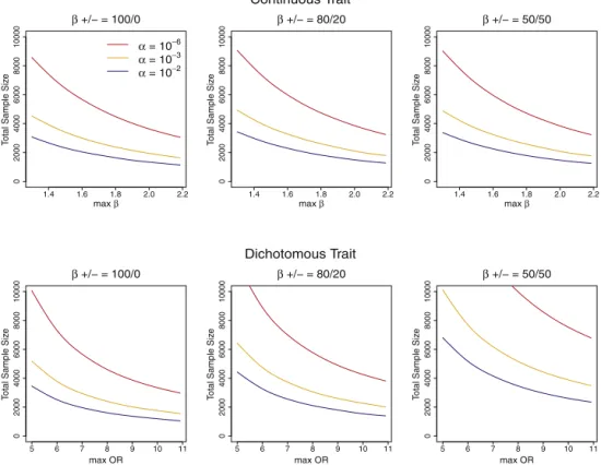
Power and Sample-Size Estimation

To illustrate our power and sample-size calculation

method, in

Figure 2

we present the estimated sample-size

curves as a function of maximum effect sizes (ORs for

dichotomous traits) necessary to detect a 30 kb region

with 5% of the variants with MAF

<

3% being causal.

Table 3

presents estimated sample sizes for several

configu-rations of practical interest. Additional sample-size curves

when causal variants are rarer (MAF

<

1%) or occur more

frequently (10% of variants are causal) or when prevalence

is varied (5%, 0.1%) can be found in

Figures S13–S15

.

These results show that, for a given region, one will

have more power (and a lower required sample size) to

detect rare causal variants if the percentage of variants

that are causal is higher, the causal rare variants have

higher MAFs and/or larger effect sizes (e.g., odds ratios

[ORs]), and the effects are more consistently in the same

direction. For case-control designs, lower prevalence

yields higher power because given the same OR and

popu-lation MAF, the lower prevalence results in enrichment of

more harmful (ORs

>

1) variants, that is higher MAFs,

across both cases and controls, that is for rarer diseases

harmful rare variants are more likely to be observed.

Conversely, if the prevalence is low, fewer protective

vari-ants (ORs

<

1), that is lower MAFs, are likely to be observed

in the sample.

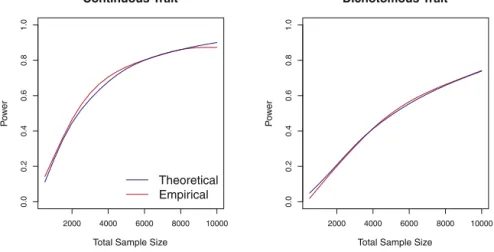
We also compared the power and sample-size formulae

estimates to the empirical, simulation-based power

esti-mates for both continuous and dichotomous traits. The

curves plotted in

Figure 3

show that the empirical power

is accurately approximated by our analytical formula.

Table 2. Characteristics of the 30 kb Region Data Sets Used in the Simulation Studies

Average Number of Observed Variants

Sample Size (n)

500 1000 2500 5000

All traits* 255 330 438 512

Continuous trait** 9.6 13.3 18.6 22.3

Dichotomous trait (b5¼100/0)** 14.4 18.7 23.5 25.2

(8)

Application to Dallas Heart Study Data

We analyzed sequence data on 93 variants in

ANGPTL3

(MIM 604774),

ANGPTL4

(MIM 605910), and

ANGPTL5

(MIM 607666) in 3476 individuals from the Dallas Heart

Study

38

to test for association between log-transformed

serum triglyceride (logTG) levels and rare variants in these

genes. We adjusted for sex and ethnicity (black, Hispanic,

or white) but did not adjust for age as a large number of

subjects have missing ages. In addition to testing for

asso-ciation via SKAT and the three burden tests considered

earlier, we also applied the permutation-based

varying-threshold method (VT) and the Polyphen-score-adjusted

VT (VTP),

16

which are based on the residuals obtained

from regressing the phenotype on the covariates and

assume gene-covariate independence. Because VT and

VTP require permutation, they are computationally

expen-sive when applied genome wide. For VTP, we used the

Polyphen score for rare variants (MAF

<

0.01) and assigned

a constant score of 0.5 to all other variants. We also

analyzed a dichotomized phenotype on the highest and

lowest quartiles of each of the six sex-ethnicity groups

(

Table 4

).

Table 3. Required Total Sample Size to Achieve 80% Power to Detect Rare Variants Associated with a Continuous or Dichotomous Case-Control Phenotype at the Genome-wide Levela¼106

Total Sample Size

Maximumb¼1.6/ Maximum OR¼5 Maximumb¼1.9/ Maximum OR¼7

5% Causal 10% Causal 5% Causal 10% Causal

Continuous trait 5,990 1,800 4,260 1,290

Dichotomous trait with prevalence 10% 15,120 4,810 9,650 3,120

Dichotomous trait with prevalence 1% 12,030 3,870 7,010 2,290

Power was estimated via the analytical formulae assuming 5% or 10% of variants with MAF<3% are causal. Regression coefficients for thescausal variants were assumed to be a decreasing function of MAF,jbjj ¼cjlog10MAFjj(j¼1,.,s), where 80% ofbj’s are positive and 20% are negative; seeFigure S2. Required total sample sizes (cases and controls) are given for different ‘‘maximum’’ effect sizes (or ORs) when MAF¼104_{and different prevalences for case-control studies.} Estimated sample sizes were averaged over 100 random 30 kb regions.

1.4 1.6 1.8 2.0 2.2

0

2000

4000

6000

8000

10000

β +/− = 100/0

max β

T

otal Sample Siz

e

α = 10−6

α = 10−3

α = 10−2

1.4 1.6 1.8 2.0 2.2

0

2000

4000

6000

8000

10000

β +/− = 80/20

max β

T

otal Sample Siz

e

1.4 1.6 1.8 2.0 2.2

0

2000

4000

6000

8000

10000

β +/− = 50/50

max β

T

otal Sample Siz

e

Continuous Trait

5 6 7 8 9 10 11

0

2000

4000

6000

8000

10000

β +/− = 100/0

max OR

T

otal Sample Siz

e

5 6 7 8 9 10 11

0

2000

4000

6000

8000

10000

β +/− = 80/20

max OR

T

otal Sample Siz

e

5 6 7 8 9 10 11

0

2000

4000

6000

8000

10000

β +/− = 50/50

max OR

T

otal Sample Siz

e

Dichotomous Trait

Figure 2. Sample Sizes Required for Reaching 80% Power

Analytically estimated sample sizes required for reaching 80% power to detect rare variants associated with a continuous (top panel) or dichotomous phenotype in case-control studies (half are cases) (bottom panel) at thea¼106, 103, and 102levels, under the assump-tion that 5% of rare variants with MAF<3% within the 30 kb regions are causal. Plots correspond to 100%, 80%, and 50% of the causal variants associated with increase in the continuous phenotype or risk of the dichotomous phenotype. Regression coefficients for thes

causal variants were assumed to be the same decreasing function of MAF as that inFigure 1. The absolute values of Required total sample sizes are plotted again the maximum effect sizes (ORs) when MAF¼104_{. Estimated total sample sizes were averaged over 100 random 30}

(9)

SKAT was by far the most powerful test for the

dichoto-mous trait. For continuous traits, SKAT has much smaller

p values than two burden methods (CAST and WST) and

VT, and has a slightly higher p value than the

counting-based burden test (N) and VTP. Note that SKAT was easier

to apply because it did not require prior functional

infor-mation (available for only a subset of variants) or

permuta-tion, and it adjusted for covariates without assuming

gene-covariate independence.

Computation Time

The computation time for the SKAT depends on the

sample size and the number of markers. To analyze a 30 kb

region sequenced on 1000, 2500, or 5000 individuals,

SKAT required 0.21, 0.73, and 2.3 s, respectively, for

continuous traits and ~20% longer for dichotomous traits,

on a 2.33 GHz laptop with 6 Gb memory. Analyzing

300 kb, 3 Mb, or 3 Gb (the entire genome) on 1000

individ-uals requires 2.5 s, 25 s, and 7 hr, respectively.

Discussion

We propose SKAT as a supervised, flexible, and

computa-tionally efficient statistical method that tests for association

between a continuous or dichotomous phenotype and rare

and common genetic variants in sequencing-based

associa-tion studies. We demonstrate that SKAT’s power is greater

than that of several burden tests over a range of genetic

models. Furthermore, we have developed analytical power

and sample-size calculations for SKAT that assist in

designing sequencing-based association studies.

2000 4000 6000 8000 10000

0.0

0.2

0.4

0.6

0.8

1.0

Continuous Trait

Total Sample Size

Po

w

e

r

Theoretical Empirical

2000 4000 6000 8000 10000

0.0

0.2

0.4

0.6

0.8

1.0

Dichotomous Trait

Total Sample Size

Po

w

e

r

Figure 3. Power Comparisons Based on

Simulation and Analytic Estimation

Power as a function of total sample size estimated by simulation with 1000 repli-cates and by the proposed power formula for continuous and dichotomous case-control traits. Simulation configurations correspond to those used inFigure 1, in which 80% of the regression coefficients for the causal rare variants were positive.

Table 4. Analysis of the Dallas Heart Study Sequencing Data

SKAT C N W VTa _VTPa

Continuous TG level 9.53105 _1.9₃₁₀3 _7.2₃₁₀5 _2.3₃₁₀4 _3.5₃₁₀4 _2.0₃₁₀5 Dichotomized TG level 1.33104 _3.2₃₁₀2 _2.2₃₁₀3 _3.1₃₁₀3 _8.6₃₁₀3 _2.1₃₁₀3 Analysis of the Dallas Heart Study sequencing data with SKAT, the weighted sum burden test (W), the counting-based burden test (N), the CAST method (C), the varying-threshold method (VT), and the Polyphen-score adjusted VT (VTP) method. Beta (1, 25) is used as the weight in the SKAT and the weighted sum test. a_{p values are estimated on the basis of 10}6_{permutations.}

Like burden tests, SKAT performs

region-based testing. However, SKAT

has several major advantages over the

existing tests. As a supervised method,

SKAT directly performs multiple

re-gressions of a phenotype on genotypes for all variants in

the region, adjusting for covariates. Hence, as with

conven-tional multiple regression models, neither direcconven-tionality

nor magnitudes of the associations are assumed a priori

but are instead estimated from the data. To test efficiently

for the joint effects of rare variants in the region on the

phenotype, SKAT assumes a distribution for the regression

coefficients of the markers, whose variances depend on

flexible weights. SKAT performs a score-based

variance-component test, whose calculation only requires fitting

the null model by regressing phenotypes on covariates

alone and computing p values analytically. The flexible

regression framework also allows us to allow for epistatic

effects.

Besides region-based analysis, SKAT can also be applied

to any biologically meaningful SNP set. As SKAT is a

regres-sion-based method, it can be easily extended to survival,

and longitudinal and multivariate phenotypes and hence

provides a comprehensive framework for a wide variety

of sequencing-based association studies.

The ability to obtain a p value directly without the need

for permutation is an attractive feature of SKAT, and allows

for rapid estimation of p values in exome and

genome-wide sequencing studies. Our simulations showed that

for continuous phenotype, the p values are accurate

when the sample size is moderate or large; for

dichoto-mous phenotypes, the p values are conservative at lower

(10)

permutations fail and require careful modifications.

Despite the conservative nature of the score test, SKAT

often still has higher power than competing methods at

small

a

levels.

SKAT can be combined with collapsing strategies to form

a hybrid testing approach. If most of the variants within

a range of allele frequencies are causal and have the same

directionality (i.e., under settings that are optimal for

burden-based tests), collapsing these variants and then

applying SKAT to the collapsed variants can improve

power. For example, because singletons are common in

sequencing studies (57 of 93 variants in the Dallas Heart

Study data), a possible hybrid strategy is to first collapse

all of the singletons into a single value and then apply

SKAT to the collapsed value and the other 36 variants.

Compared to the original SKAT, this strategy gives a slightly

lower p value, 3.1

3

10

5

, for the continuous trait and

a slightly higher p value, 1.6

3

10

4

, for the dichotomous

trait. Simulation studies showed that the two methods are

of similar power under the settings we used to generate

Figure 1

.

An important feature of SKAT is that it allows for

incor-poration of flexible weight functions to boost analysis

power, for example by increasing the weight of variants

with lower MAFs and decreasing the weight of information

from variants inferred with lower confidence. Good

choices of weights are likely to improve the power of the

association test with SKAT, although simulations show

that even equal weights can yield high power when

combined with thresholding. In our simulation studies,

we employed a class of flexible continuous weights as

a function of MAF by using the beta function, which

increases the weight of rare variants and does not require

thresholding. Users can define other types of weight

func-tions. To further improve analysis power, one can estimate

weights by incorporating information besides MAF, for

example by using the Polyphen score or integrating other

annotation information, which will become increasingly

available as our understanding of genome variation

improves. Therefore, because of its flexibility, SKAT has

the capacity to mature, and its power to increase, as the

field progresses.

Appendix A

Estimating the Null Distribution for Q

Under the null hypothesis,

Q

follows a mixture of

chi-square distributions.

29,30

_{More specifically, we define}

_P

0

¼

V

X

~

ð

X

~

0

V

X

~

Þ

1

_X

~

0

_V

_where

_X

~

_{is the}

_n

₃

_(p

_þ

_{1) matrix}

equal to [

1 ,

X

]. For continuous phenotypes,

V

¼

b

s

2₀

I

where

b

s

0

is the estimator of

s

under the null model where

f(

G

)

¼

0, and

I

is an

n

3 n

identity matrix. For

dichoto-mous phenotypes,

V

¼

diag

ð

m

b

01ð

1 m

b

01Þ;

b

m

02ð

1 b

m

02Þ;

.

;

b

m

0n

ð

1 b

m

0n

ÞÞ

where

m

b

0i

¼

logit

1

ð

b

a

þ

b

a

0

X

i

Þ

is the

esti-mated probability that the

i-th subject is a case under the

null model. Then under the null model

Q

X

n

i¼1

l

i

c

2₁_;i

;

(Equation 6)

where (

l

1

,

l

2

,

.

,

l

n

) are the eigenvalues of

P

1=20

KP

1=2 0

, and

c

2

1;i

are independent

c

21

random variables.

Several approximation and exact methods have been

suggested to obtain the distribution of

Q.

39

Among these,

the Davies exact method,

26

based on inverting the

charac-teristic function of

Equation 6

, appears to work well in

practice and is used here.

SKAT Is a Generalization of the C-Alpha Test

The recently proposed the C-alpha test has advantages

over burden tests in that it explicitly models the possibility

that minor alleles can be deleterious or protective.

However, it does not currently allow for the analysis of

quantitative outcomes or the inclusion of covariates and

p value calculation requires permutation. We demonstrate

that for a dichotomous trait in the absence of covariates,

the C-alpha test statistic is equivalent to the SKAT statistic

with unweighted linear kernel, which is the same as the

kernel machine test in Wu et al.

24

Suppose the

j-th variant is observed

d

j

times in the cases,

out of

n

j

times total in cases and controls, and that

p

0

¼

P

n

i¼1

y

i

=

n. For a dichotomous trait and no covariates,

the C-alpha test statistic

T

a

¼

X

p

j¼1

h

d

j

n

j

p

0

2

n

j

p

0

1 p

0

i

(Equation 7)

Denote

T

1 a

¼

P

p

j¼1

ð

d

j

n

j

p

0Þ2

. Because

P

p

j¼1

n

j

p

0ð

1 p

0Þ

is the mean of

T

a

under the null hypothesis of no

associa-tion,

T

1

a

is the C-alpha test statistic without mean centering.

Because

d

j

¼

y

0

G

:

j

and

n

j

¼

J

0

G

:

j

, where

G

:

j

is the

j-th

column of the genotype matrix

G

and

J

¼ ð

1 ;

.

;

1 Þ

0

, it

can be easily shown that

T

_a1

¼

y

p

0

J

0

GG

0

_y

_p

0

J

:

(Equation 8)

Note that under the unweighted linear kernel,

K

¼

GG

’

and

b

m0

¼

p

0

J

if no covariates are present. Hence,

Equation

8 is identical to

Equation 3

, that is

T

1

a

is equivalent to the

SKAT test statistic with unweighted linear kernel.

(11)

Supplemental Data

Supplemental Data include 15 figures and can be found with this article online athttp://www.cell.com/AJHG/.

Acknowledgments

This work was supported by grants P30 ES010126 (to M.C.W.), DMS 0854970 and R01 GM079330 (to T.C.), R01 HG000376 (to M.B.), and R37 CA076404 and P01 CA134294 (to S.L. and X.L.). We thank Jonathan Cohen, Alkes Price, and Shamil Sunyaev for providing the Dallas Heart Study data and Larisa Miropolsky for help with the software development.

Received: March 16, 2011 Revised: May 27, 2011 Accepted: May 30, 2011 Published online: July 7, 2011

Web Resources

The URLs for data presented herein are as follows:

1000 Genomes Project,http://www.1000genomes.org/

Online Mendelian Inhereitance in Man (OMIM), http://www. omim.org

SKAT software,http://www.hsph.harvard.edu/~xlin/software.html

References

1. Hindorff, L.A., Sethupathy, P., Junkins, H.A., Ramos, E.M., Mehta, J.P., Collins, F.S., and Manolio, T.A. (2009). Potential etiologic and functional implications of genome-wide associa-tion loci for human diseases and traits. Proc. Natl. Acad. Sci. USA106, 9362–9367.

2. Margulies, M., Egholm, M., Altman, W.E., Attiya, S., Bader, J.S., Bemben, L.A., Berka, J., Braverman, M.S., Chen, Y.J., Chen, Z., et al. (2005). Genome sequencing in microfabricated high-density picolitre reactors. Nature437, 376–380.

3. Mardis, E.R. (2008). Next-generation DNA sequencing methods. Annu. Rev. Genomics Hum. Genet.9, 387–402. 4. Ansorge, W.J. (2009). Next-generation DNA sequencing

tech-niques. New Biotechnol.25, 195–203.

5. Eichler, E.E., Flint, J., Gibson, G., Kong, A., Leal, S.M., Moore, J.H., and Nadeau, J.H. (2010). Missing heritability and strategies for finding the underlying causes of complex disease. Nat. Rev. Genet.11, 446–450.

6. Ley, T.J., Mardis, E.R., Ding, L., Fulton, B., McLellan, M.D., Chen, K., Dooling, D., Dunford-Shore, B.H., McGrath, S., Hickenbotham, M., et al. (2008). DNA sequencing of a cytoge-netically normal acute myeloid leukaemia genome. Nature

456, 66–72.

7. Li, H., Ruan, J., and Durbin, R. (2008). Mapping short DNA sequencing reads and calling variants using mapping quality scores. Genome Res.18, 1851–1858.

8. Li, R.Q., Li, Y.R., Fang, X.D., Yang, H.M., Wang, J., Kristiansen, K., and Wang, J. (2009). SNP detection for massively parallel whole-genome resequencing. Genome Res.19, 1124–1132.

9. Bansal, V., Harismendy, O., Tewhey, R., Murray, S.S., Schork, N.J., Topol, E.J., and Frazer, K.A. (2010). Accurate detection and genotyping of SNPs utilizing population sequencing data. Genome Res.20, 537–545.

10. Carvajal-Carmona, L.G. (2010). Challenges in the identifica-tion and use of rare disease-associated predisposiidentifica-tion variants. Curr. Opin. Genet. Dev.20, 277–281.

11. Schork, N.J., Murray, S.S., Frazer, K.A., and Topol, E.J. (2009). Common vs. rare allele hypotheses for complex diseases. Curr. Opin. Genet. Dev.19, 212–219.

12. Li, B., and Leal, S.M. (2008). Methods for detecting associa-tions with rare variants for common diseases: application to analysis of sequence data. Am. J. Hum. Genet.83, 311–321. 13. Madsen, B.E., and Browning, S.R. (2009). A groupwise associ-ation test for rare mutassoci-ations using a weighted sum statistic. PLoS Genet.5, e1000384.

14. Morgenthaler, S., and Thilly, W.G. (2007). A strategy to discover genes that carry multi-allelic or mono-allelic risk for common diseases: a cohort allelic sums test (CAST). Mutat. Res.615, 28–56.

15. Li, B., and Leal, S.M. (2009). Discovery of rare variants via sequencing: implications for the design of complex trait asso-ciation studies. PLoS Genet.5, e1000481.

16. Price, A.L., Kryukov, G.V., de Bakker, P.I., Purcell, S.M., Staples, J., Wei, L.J., and Sunyaev, S.R. (2010). Pooled association tests for rare variants in exon-resequencing studies. Am. J. Hum. Genet.86, 832–838.

17. Han, F., and Pan, W. (2010). A data-adaptive sum test for disease association with multiple common or rare variants. Hum. Hered.70, 42–54.

18. Morris, A.P., and Zeggini, E. (2010). An evaluation of statistical approaches to rare variant analysis in genetic association studies. Genet. Epidemiol.34, 188–193.

19. Zawistowski, M., Gopalakrishnan, S., Ding, J., Li, Y., Grimm, S., and Zo¨llner, S. (2010). Extending rare-variant testing strategies: analysis of noncoding sequence and imputed genotypes. Am. J. Hum. Genet.87, 604–617.

20. Asimit, J., and Zeggini, E. (2010). Rare variant association anal-ysis methods for complex traits. Annu. Rev. Genet.44, 293–308. 21. Neale, B.M., Rivas, M.A., Voight, B.F., Altshuler, D., Devlin, B., Orho-Melander, M., Kathiresan, S., Purcell, S.M., Roeder, K., and Daly, M.J. (2011). Testing for an unusual distribution of rare variants. PLoS Genet.7, e1001322.

22. Price, A.L., Patterson, N.J., Plenge, R.M., Weinblatt, M.E., Shadick, N.A., and Reich, D. (2006). Principal components analysis corrects for stratification in genome-wide association studies. Nat. Genet.38, 904–909.

23. Kwee, L.C., Liu, D., Lin, X., Ghosh, D., and Epstein, M.P. (2008). A powerful and flexible multilocus association test for quantitative traits. Am. J. Hum. Genet.82, 386–397. 24. Wu, M.C., Kraft, P., Epstein, M.P., Taylor, D.M., Chanock, S.J.,

Hunter, D.J., and Lin, X. (2010). Powerful SNP-set analysis for case-control genome-wide association studies. Am. J. Hum. Genet.86, 929–942.

25. Lin, X. (1997). Variance component testing in generalised linear models with random effects. Biometrika84, 309–326. 26. Davies, R. (1980). The distribution of a linear combination of

chi-square random variables. J. R. Stat. Soc. Ser. C Appl. Stat.

29, 323–333.

27. Pan, W. (2009). Asymptotic tests of association with multiple SNPs in linkage disequilibrium. Genet. Epidemiol.33, 497–507. 28. Cristianini, N., and Shawe-Taylor, J. (2000). An Introduction to Support Vector Machines and Other Kernel-Based Learning Methods (Cambridge: Cambridge Univ Press).

(12)

kernel machines and linear mixed models. Biometrics 63, 1079–1088.

30. Liu, D., Ghosh, D., and Lin, X. (2008). Estimation and testing for the effect of a genetic pathway on a disease outcome using logistic kernel machine regression via logistic mixed models. BMC Bioinformatics9, 292.

31. Fleuret, F., and Sahbi, H. (2003). Scale-invariance of support vector machines based on the triangular kernel. In 3rd Inter-national Workshop on Statistical and Computational Theories of Vision. (ftp://ftp.inria.fr/INRIA/publication/publi-pdf/RR/ RR-4601.pdf).

32. Ramensky, V., Bork, P., and Sunyaev, S. (2002). Human non-synonymous SNPs: server and survey. Nucleic Acids Res.30, 3894–3900.

33. Kumar, P., Henikoff, S., and Ng, P.C. (2009). Predicting the effects of coding non-synonymous variants on protein func-tion using the SIFT algorithm. Nat. Protoc.4, 1073–1081. 34. Liu, H., Tang, Y., and Zhang, H. (2009). A new chi-square

approximation to the distribution of non-negative definite quadratic forms in non-central normal variables. Comput. Stat. Data Anal.53, 853–856.

35. Lee, S., Wu, M.C., Cai, T., Li, Y., Boehnke, M., and Lin, X. (2011). Power and sample size calculations for designing rare variant sequencing association studies. In Harvard University Technical Report. (http://www.hsph.harvard.edu/~xlin). 36. Durbin, R.M., Abecasis, G.R., Altshuler, D.L., Auton, A.,

Brooks, L.D., Gibbs, R.A., Hurles, M.E., and McVean, G.A.; 1000 Genomes Project Consortium. (2010). A map of human genome variation from population-scale sequencing. Nature

467, 1061–1073.

37. Schaffner, S.F., Foo, C., Gabriel, S., Reich, D., Daly, M.J., and Altshuler, D. (2005). Calibrating a coalescent simulation of human genome sequence variation. Genome Res.15, 1576– 1583.

38. Romeo, S., Yin, W., Kozlitina, J., Pennacchio, L.A., Boerwinkle, E., Hobbs, H.H., and Cohen, J.C. (2009). Rare loss-of-function mutations in ANGPTL family members contribute to plasma triglyceride levels in humans. J. Clin. Invest.119, 70–79. 39. Duchesne, P., and Lafaye De Micheaux, P. (2010). Computing