Optimal Allocation of Ships to Quay Length in Container Ports

(1)

Vol. 3, No. 4, pp 275-290 Winter 2010

Optimal Allocation of Ships to Quay Length in Container Ports

H. Javanshir1∗, S.R.Seyed-Alizadeh Ganji2

1

Assistant Professor, Dep. of Industrial Engineering, Islamic Azad University, South Tehran Branch, Iran [email protected]

2

M. Sc., Dep. of Transportation Engineering, Islamic Azad University, Science and Research Branch, Iran [email protected]

ABSTRACT

Due to the continuously increasing container trade, many terminals are presently operating at or close to capacity. An efficient terminal is one that facilitates the quick transshipment of containers to and from ships. In this sake, this paper addresses the ship assignments problem at a maritime container terminal, where ships are normally assigned to specific quay cranes until the work is finished. The paper’s target is to develop a new Continues Berth Allocation Problem (CBAP) in the form of a mixed integer nonlinear programming to achieve the best service time in a container terminal. For illustrating the accuracy of Proposed model (PM), Imai et. al. 's model (IM) (TRANSPORT RES B, 39 (2005) 199–221) was applied and a wide variety of computational test examples were conducted. The results of demonstrated that the presented BAPC reduces the number of nonlinear variables (constraints) and generates substantial savings in the CPU time.

Keywords: Optimal transportation, Continues Berth allocation Problem (CBAP), mixed integer nonlinear programming

1. INTRODUCTION

Container terminals are essential inter-modal transportation network which work under multiple operational objectives. The main one is to minimize ships turnaround time (including serving time and waiting time) and subsequently maximize the terminal throughput. They can be achieved by efficient loading and discharging of ships. Therefore, accurate ship assignment is usually taken as the key performance measure for the operational efficiency of a terminal.

At a multi-user terminal, ships are usually berthed relatively close to their container storage in the yard for quicker container transshipment to and from the ships. However, in order to increase the usage of quay space in berthing ships, some ships may be assigned to a quay location far from their container storage. Optimum assignment of arrived ships to quay length is one of the most important

factors to reduce the sum of ships turnaround time. So, this paper tries to consider the Continues

Berth Allocation Problem (CBAP) to achieve higher productivity in ship berthing. The Proposed

model (PM) is able to reflect the abilities of Imai et al. (2005)'s model (IM) in less solution time. To

∗

(2)

solve the model Branch and Bound (B & B) algorithm has been used. The rest of the paper is organized as follows:

The next section provides a literature review on the Berth Allocation Problem (BAP). Section 3,

describes the model formulation. In section 4, a variety of computational experiments are conducted which demonstrate the efficiency of PM in decreasing computational time against IM. Section 6 provide the analysis of CBAP results and the final section concludes the paper.

2. LITERATURE REVIEW

Many researches have been conducted to increase the efficiency of container terminals operation. Different subjects of these researches include berth allocation problem (Brown et al. (1994), Brown et al. (1997), Guan et al. (2002), Imai et al. (1997), Imai et al. (2001), Imai et al. (2003), Imai et al. (2007), Imai et al. (2005), Kim and Moon (2003), Lai and Shih (1992), Li et al. (1998), Lim (1998), Nishimura et al. (2001), Park and Kim (2002), Park and Kim (2003), Ganji et al. (2009)); quay and yard cranes assignment (Javanshir and Ganji (2010), Tavakkoli-Moghaddam et al. (2009); yard storage management (Zhang et al. (2003)) Recently a unique classification of a paper is not possible according to the given information, the best fit of classifying attributes is taken in Vis and Koster (2003) and Bierwirth and Meisel (2010). Studies that have been focused on assignment of ships to berths are considered in detail.

Lai and Shih (1992) have used a First-Come- First-Served (FCFS) allocation rule in the form of a heuristic algorithm for analysis of the BAP. Brown et al. (1994, 1997) proposed the first mathematical models of BAP to maximize the sum of benefits for ships in naval port. Imai et al.

(1997) address a Discrete Berth Allocation Problem (DBAP) in the static variant for commercial

ports. In this problem, the assignment and sequencing of ships to berths is searched with respect to minimum waiting and handling times of the ships. A Lagrangean relaxation based heuristic is presented to solve the problem. Dynamic variant of the DBAP is considered by Imai et al. (2001) with regard to the port stay times of ships. They extended the static version of the DBAP presented into a dynamic treatment with only one objective named berth performance (Imai et al. 1997). A heuristic solution based on the sub gradient method with Lagrangian relaxation was developed to solve the model. Multi-water depth configuration of DBAP in Imai et al. (2001) is conducted by Nishimura et al. (2001). They proposed a genetic meta-heuristic solution method for solving that problem.

Another type of approach to the BAP is proposed in recent studies is the one with a continuous location called CBAP. Lim (1998) was the first to consider a berth as a continuous line and viewed the berth planning problem as a two-dimensional bin packing problem. He discussed how to locate berthing positions of ships so that the throughput of the berth is maximized, but did not consider the berthing time as a decision variable. The static CBAP with fixed ships handling time has been introduced by Li et al. (1998). The problem is formulated as a ‘‘multiple-job-on-one-processor” scheduling problem. This allows adapting the First-Fit-Decreasing heuristic, well-known from bin packing, for minimizing the maximum completion time among the ships. Guan et al. (2002) proposed an m-parallel machine scheduling formulation and developed a heuristic was developed for the CBAP to minimize the total weighted completion time of the ships. Park and Kim (2002) introduced the first model for the CBAP to determine simultaneously the berthing time and position for each ship with the objective of minimizing the costs resulting from delayed ships departures. The authors proposed a sub-gradient optimization technique. Kim and Moon (2003) solved the same CBAP as the one proposed by Park and Kim (2002) with the simulated annealing method. Park and Kim (2003) determine the optimal start times of ship service and associated mooring

(3)

locations and at the same time they determine the optimal assignment of quay cranes to those ships. In their study, the handling time for a particular ship is a function of the number of quay cranes engaged in the ship, however, the handling time is independent from the mooring location of the ship. Imai et al. (2005) proposed an integer nonlinear mathematical model for CBAP. They assume that a ship’s handling time depends on the quay location where the particular ship is handled. IM is presented in Appendix A. Recently, Imai et al. (2007) addressed the berth BAP at a multi-user container terminal with indented berths for fast handling of mega-containerships. They constructed a new integer linear programming formulation and then the formulation is extended to model the BAP at a terminal with indented berths, where both mega-containerships and feeder ships are to be served for higher berth productivity. The BAP at the indented berths is solved by genetic algorithm. 3. MATHEMATICAL FORMULATION

This section proposes a new mathematical formulation of CBAP. The assumptions in this model are as follow:

• There is no delay in ship arrival.

• Ships handling time increases linearly and with a slope of

γ

_i

≥

0

. So, the handling time of a

ship can be defined as follow (Imai et al. (2005)):

i i i i

i CM p M

C = + −

γ

Where

CM

_i is the handling time of the ship i in the best berthing location

M

_i and

γ

_i depends on

quality port's internal equipments function.

• The required gap between adjacent ships for anchoring is considered in the length of ships.

• Elapsed time of ships berthing is considered in handling time of ships.

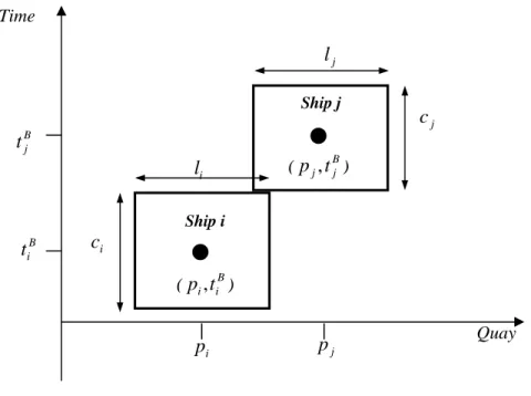
As illustrated in Figure 1, the problem is set in a 2-dimensional space, the berth length and the planning time defining the horizontal and vertical axes, respectively. We can represent a ship geometrically by a rectangle, such that the length of the rectangle is the length of the ship and the height of the rectangle is the duration of its stay (or handling time). The bottom edge of the rectangle represents the start time of handling the ship. The top edge represents the completion time of handling the ship (or the departure time of the ship). The quay space can be represented geometrically by an infinitely long rectangle where its length is the quay length and the height defines the time.

The following notations are used for a mathematical formulation.

Indices:

v

T

j

i

,

(

=

1 ,...,

)

∈

Number of ships to be allocated in the quay

Problem data:

(4)

i

a

: Arrival time of ship i;

i

l

: The length of ship i.

i

M

: Best berthing location of ship i. This location is represented by the center of ship i at the

horizontal axis (Quay length axis);

i

γ

: Additional travel cost of handling containers from or to ship i resulting from non-optimal

berthing locations;

m: A sufficiently large constant;

Decision variables:

i

p

: Berthing location of ship i (is integer);

B i

t

: Berthing time of ship i;

x ij

δ

: 1, if ship i is located to the left of ship j in the time-berth-length space; 0, otherwise;

y ij

δ

: 1, if ship i is located below ship j in the time-berth-length space; 0, otherwise; Where

p

_is and

t

_iBs are variables and

p

_i s are integers.

The CBAP can be formulated as follows:

Minimize

∑

{

}

=

−

×

+

v

i

i i i i i B

i

CM

p

M

a

t

1

γ

(1)

Subject to:

(

)

(

x

)

ij j

j i

i

p

m

l

p

+

≤

+

1 −

δ

2

j =1,2,...,v,

i

≠

j

(2)

(

)

(

y

)

ij B

j i B

i

c

t

m

t

+

≤

+

1 −

δ

i, j=1,2,...,v,

i

≠

j

(3)

1 ≥

+

y

ji y ij x ji x

ij

δ

i, j=1,2,...,v,

i

<

j

(4)

Q

l

p

i

+

≤

2

i=1,2,...,v (5)

2 i i

l

(5)

i B

i

a

t

≥

i=1,2,...,v (7)

0 ≥

i

p

i=1,2,...,v (8)

The objective function (1) is the sum of service times for all ships, where the service time is defined as the time spent from arrival to departure including the waiting time for a quay space to become available. Constraints (2)–(3) are the non-overlapping restriction. Note that as either quay-non-overlapping or time-non-quay-non-overlapping should be satisfied, therefore

δ

_ijx

+

δ

_jix

+

δ

_ijy

+

δ

_jiy

−

1 ≥

0

in constraint (4). Constraints (5) and (6) ensure that every ship must be berthed within the quay length. Constraint (7) assures that the ships are berthed after their arrival.

4. NUMERICAL EXPERIMENTS

The solution procedure is coded in ‘‘LINGO’’ software on a personal computer Pentium IV 2.8 GHz PC with 512MB RAM). We developed five basic problems with different quay lengths (from 600 to 2400) and numbers of ships 6, 7 and 8 in a day. For each basic problem, we set up different best handling times and one rate of increase in handling time as additional cost factor. The data sets are generated with average ship sizes of 200, 250, 300, 400 and 500 meters. The average best handling time per ship at the best quay location for the data sets is 7, 9, 10, 11and 13 hours, respectively. The ship arrival pattern follows the uniform distribution with average interval of 7, 10, 13, 15 and 18 hours. The best berthing location are in the distances of 0.25, 0.50, 0.75 length of quay repeated in order to arriving ships. In addition, every groups of an example is conducted with different additional cost factors 0.005, 0.05, 0.1, 0.08 and 0.2. Different data sets are given in Table 1.

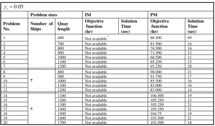
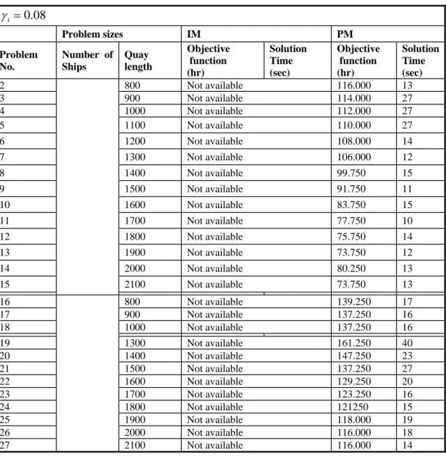
Comparison between Imai's and PMs on the number of variables and the computational time are presented in Tables 2-7. As shown in Table 2, there are less non linear variables and constraints in

the PM than their similar states in IM. The number of nonlinear terms ( p_i −M_i ) in the PM which

is occurred in objective functions is equal 1. This amount is up to 120 constraints for IM. So, it is clear that less operation time is needed for PM rather than that one can be expected for Imai's model.

According to Tables 4-7, we can find the computational time of problem using the PM is much less than the similar one by opponent model. In many instances, the PM was able to solve more complex problem with less quay length or more amount of additional cost against other similar ones. This means that the sensitivity of IM against the increase of the problem's dimension is more than the sensitivity of PM. In the other word, there are lots of problems which might not be not solved by IM could be analyzed using the PM. Some of these unsolvable instances, of course, in acceptable running time (less than 1200 seconds), are referred in Tables 3-7. In Table 3, examples with 6 ships in a day and the quay length less than 1000 meters, 7 ships in a day and the quay length less than 1300 meters, and 8 ships in a day and the quay length less than 1600 meters are unsolvable using IM. In addition, among 93 instances in Tables 4-7 were solved by IM in acceptable solution time

which is with 6 ships, quay length 1300 m and

γ

_i

=

0 .

1

. It is necessary to mention that these

examples were solved in much more time than solving those ones by PM. From these tables we can easily understand that problems will become more complex to solve by increasing in the amount of additional cost.

(6)

5. RESULTS AND DISCUSSIONS

In this section we consider the output of five selected samples mentioned above in detail. These samples data are as follow:

1. 8 ships, quay length 1200 m with

γ

_i

=

0 .

005

(Data set 1)

γ

_i

=

0 .

05

(Data set 2)

γ

_i

=

0 .

1

(Data set 3)

γ

_i

=

0 .

08

(Data set 4)

γ

_i

=

0 .

2

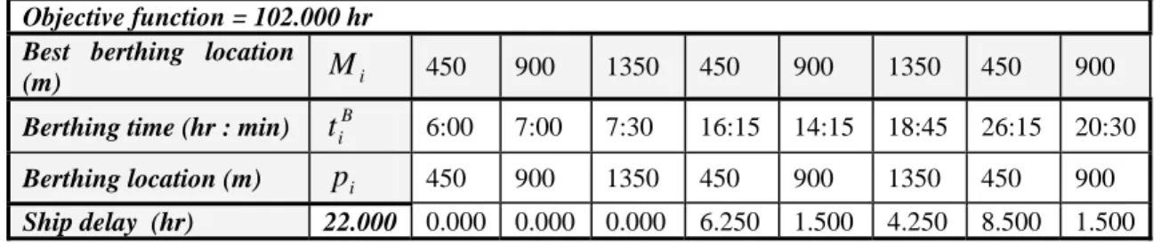
(Data set 5)

The results of Samples 1, 2, 3, 4 and 5 can be observed in Table 8-12, respectively. The Outputs

include the berthing time (

t

iB), the berthing location (

p

i) of each ship. Moreover, the measure of

every ship's delay is represented in these tables.

Results in Table 8 illustrates all ships except the second ship berthed in the best location exactly at the arriving time are located in the quayside with related delays. The delay amount of ships in this assumed port (5.125 hours) includes 9% of objective function. Whole ships except final ship are at arriving time. We can find similar results in Tables 9-12.

Figure 2 shows the changes of objective function against the quay length for the problem with 8

ships and

γ

_i

=

0 .

005

. Critical intervals in this diagram are between 940-950 and 1180-1200 meters.

Reduction of objective function in these intervals is completely considerable. The important point is that the descending process of objective function's amount for the lengths more than 1500 meters, in above diagram, remains constant in its minimum amount, 58 hours.

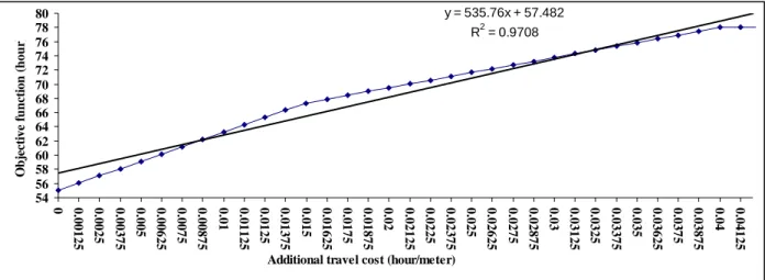
Figure 3, illustrates the changes of objective function of 8 ships for the length of quay 1200 meters

against different amount of

γ

_i. As observed in this figure, the amount of objective function

for

γ

_i

=

0 .

04

is about 78.00 hours that reduces by the linear reduction of

γ

_i with regression

coefficient

r

2

=

0 .

97

. In this figure, the notable point is that with reduction of

γ

i from 0.005 to

0.000, the amount of objective function with about 4 hours reduction reaches to about 55 hours.

However, if

γ

i

=

0 .

04

, the amounts of objective function with about 23 hours increase reaches to

about 78 hours. It means we can decrease ship's turnaround time to maximum 23 hours only by adequate allocation of the container storages or the correct timing of handling tools. Similar results could be found for other samples that we disregard mentioning about them.

6. CONCLUSION

The Presented Model (PI) in this paper has been formulated based on the existing concepts in berth allocation problems continuously that have less integer and nonlinear variables rather than the presented model by Imai in 2005. Using PI can cause better analysis of the BAP in a more

(7)

acceptable computational time. After presenting five various examples, two effective parameters in efficiency of container ports that is the length of quay and coefficient of handling time increasing (to the distance from the best berthing location) were reviewed as sensitivity analysis. According to these results, adequate allocation of container storages and also automation of handling process (simultaneous crane scheduling and trailers, use of multi-trailers systems, etc) can be proposed in the increasing of efficiency of containers port as the cheep alternatives, rather the construction and development alternatives.

REFERENCES

[1] Brown G.G., Lawphongpanich S., Thurman K.P. (1994), Optimizing ship berthing; Naval Research Logistics 41; 1–15.

[2] Brown G.G., Cormican K.J., Lawphongpanich S., Widdis D.B. (1997), Optimizing submarine berthing with a persistence incentive; Naval Research Logistics 44; 301–318.

[3] Guan Y., Xiao W.-Q., Chueng R.K., Li C.-L. (2002), A multiprocessor task scheduling model for berth allocation: Heuristic and worst case analysis; Operations Research Letter 30; 343–350.

[4] Imai A., Nagaiwa K., Chan W.T. (1997), Efficient planning of berth allocation for container terminals in Asia; Journal of Advanced Transportation 31; 75–94.

[5] Imai A., Nishimura E., Papadimitriou S. (2001), The dynamic berth allocation problem for a container port; Transportation Research Part B 35; 401–417.

[6] Imai A., Nishimura E., Papadimitriou S. (2003), Berth allocation with service priority; Transportation Research Part B 37; 437–457.

[7] Imai A., Nishimura E., Hattori M., Papadimitriou S. (2007), Berth allocation at indented berths for mega-containerships; European Journal of Operational Research 179(2); 579-593.

[8] Imai A., Sun X., Nishimura E., Papadimitriou S. (2005), Berth allocation in a container port: Using a continuous location space approach; Transportation Research Part B 39; 199–221.

[9] Kim K.H., Moon K.C. (2003), Berth scheduling by simulated annealing; Transportation Research Part B 37; 541–560.

[10] Lai K.K., Shih K. (1992), A study of container berth allocation; Journal of Advanced Transportation 26; 45–60.

[11] Li C.-L., Cai X., Lee C.-Y. (1998), Scheduling with multiple-job-on-one-processor pattern; IIE Transactions 30; 433–445.

[12] Lim A. (1998), The berth planning problem; Operations Research Letters 22; 105–110.

[13] Nishimura E., Imai A., Papadimitriou S. (2001), Berth allocation planning in the public berth system by genetic algorithms; European Journal of Operational Research 131; 282–292.

[14] Park K.T., Kim K.H. (2002), Berth scheduling for container terminals by using a sub-gradient optimization technique; Journal of the Operational Research Society 53; 1054–1062.

(8)

[16] Seyedalizadeh-Ganji S.R., Javanshir H., Vaseghi F. (2009), Nonlinear Mathematical Programming for Optimal Management of Container Terminals; International Journal of Modern Physics B 23(27); 5333-5342.

[17] Javanshir H., Seyedalizadeh-Ganji S.R. (2010), Yard crane scheduling in port container terminals using genetic algorithm; Journal of Industrial Engineering International; In Press.

[18] Tavakkoli-Moghaddam R., Makui A., Salahi S., Bazzazi M., Taheri F. (2009), An efficient algorithm for solving a new mathematical model for a quay crane scheduling problem in container ports; Computers and Industrial Engineering 56(1); 241–248.

[19] Zhang C., Liu J., Wan Y.-W., Murty K.G., Linn R. (2003), Storage Space Allocation in Container Terminals; Transportation Research Part B: Methodology 37B(10); 883–903.

[20] Vis I.F.A., Koster R.D. (2003), Transshipment of containers at a container terminal: An overview; European Journal of Operational Research 147; 1–16.

[21] Bierwirth C., Meisel F. (2010), A survey of berth allocation and quay crane scheduling problems in container terminals; European Journal of Operational Research202; 615-627.

Appendix A. (IM)

The formulation is based on the following notations:

V

T

i

(

=

1 ,...,

)

∈

: Set of ships,

i

A

: Estimated arrival time of ship i,

i

L

: Length of ship i (including the inter-ship clearance distance),

Q

: Length of quay,

i

M

: Berthing location with the minimum handling time of ship i (

L

_i

2 ≤

M

_i

≤

Q

−

L

_i

2

),

i

M

C

: Handling time of ship i in

M

i;

i

α

: Additional travel cost

i

C

: Handling time of ship i, Ci =CM_i + pi−Mi

α

i

p

: Berthing location of ship i; B

i

t

: Start time of handling for ship i, and

F B

i i i

(9)

Where

p

_i and B i

t

are variables and integer. The BAPC was formulated as follows:

[P]

=

∑

_∈

(

−

)

V

i i

F

i

A

t

Z

Min

(1)

Subject to p

ij j i p ij j i

L

p

δ

2 +

≥

−

∀

i

,

j

(

≠

i

)

∈

V

,

(2)

t ij j i t ij F j B j F i B

i

t

C

t

_δ

2

2 +

≥

+

−

+

,

)

(

,

j

i

V

i

≠

∈

∀

(3)

1 ≥

+

t

ij p

ij

δ

∀

i

,

j

(

≠

i

)

∈

V

,

(4)

0

2 ≥

−

i i

L

p

∀

i

∈

V

,

(5)

Q L

p_i + i ≤

2

∀

i

∈

V

,

(6)

)

0 ,

max(

_i

B

i

A

t

≥

∀

i

∈

V

,

(7)

i B i F

i

t

C

t

=

+

∀

i

∈

V

,

(8)

0 ,

B

≥

i i

t

p

and are integer

∀

i

∈

V

,

(9)

}

1 ,

0 {

,

t

∈

ij p ij

δ

∀

i

,

j

(

≠

i

)

∈

V

,

(10)

Where

δ

_ijp and t ij

δ

are the variables defined as :

1 :

=

p ij

δ

if non-overlapping restriction in quay axis is applied for ships i and j,

=0 Otherwise.

1 :

=

t ij

δ

if non-overlapping restriction in time axis is applied for ships i and j,

(10)

Table 1 Different data sets Ship lengths Ship 8 Ship 7 Ship 6 Ship 5 Ship 4 Ship 3 Ship 2 Ship 1 200 150 250 200 150 250 200 150

Data sets 1

300 300 200 250 250 200 300 200

Data sets 2

400 450 400 200 350 400 250 350

Data sets 3

400 450 350 500 300 400 550 250

Data sets 4

600 550 350 600 550 450 500 400

Data sets 5

Best handling times

7.00 5.00 9.00 7.00 5.00 9.00 7.00 5.00

Data sets 1

11.00 10.50 7.25 8.50 8.00 7. 50 11.50 7.75

Data sets 2

11.75 12.25 11.00 6.25 10.00 11.25 7.25 10.25

Data sets 3

13.00 13.50 7.75 13.50 7.25 12.75 14.25 6.00

Data sets 4

14.75 14.00 7.75 15.00 14.25 13.00 13.75 11.50

Data sets 5

arrival time to the port (hr: min)

13:00 12:00 11:00 10:00 9:00 8:00 7:00 6:00

Data sets 1

16:00 14:30 13:00 11:00 9:45 8:30 7:15 6:00

Data sets 2

19:00 17:45 14:30 12:45 10:00 7:30 7:00 6:00

Data sets 3

21:00 19:30 18:15 15:45 13:00 10:30 8:45 6:00

Data sets 4

23:00 21:15 18:30 16:15 12:15 11:45 9:00 6:00

Data sets 5

Quay Ship i ) B i i

t

p

,

( i

p

B i

t

B j t i

c

j

c

j

p

j

l

i

l

Figure 1 Structure of CBAP

Time Ship j ) B j j t p , (

(11)

Table 2 The sizes of Imai and PMs for problems with 6, 7 and 8 ships Number of nonlinear constraints Number of nonlinear variables Number of nonlinear constraints Number of nonlinear variables Number of Ships 1 6 66 84 6 1 7 91 112 7 1 8 120 144 8

Table 3 The results of the computational experiment for set data 1

005 .

0 =

i

γ

PM IM Problem sizes Solution Time (sec) Objective function (hr) Solution Time (sec) Objective function (hr) Quay length Number of Ships Problem No. 26 54.500

Not available* 700 1 16 49.750 Not available 800 2 15 49.000 Not available 900 3 15 48.250 Not available 1000 4 13 46.500 194 46.500 1100 5 13 45.750 93 45.750 1200 6 13 45.000 45 45.000 1300 7 13 45.000 30 45.000 1400 6 8 26 58.125 Not available 800 9 26 56.500 Not available 900 10 20 53.375 Not available 1000 11 15 53.000 Not available 1100 12 15 51.125 Not available 1200 13 14 50.000 291 50.000 1300 14 14 50.000 48 50.000 1400 15 7 77 63.625 Not available 1000 16 44 62.500 Not available 1100 17 24 59.125 Not available 1200 18 17 58.250 Not available 1300 19 13 58.125 Not available 1400 20 15 58.000 Not available 1500 21 12 58.000 771 58.000 1600 22 12 58.000 563 58.000 1700 8 23 *

(12)

05 .

0 =

i

γ

PM IM Problem sizes Solution Time (sec) Objective function (hr) Solution Time (sec) Objective function (hr) Quay length Number of Ships Problem No. 69 88.500

Not available* 600 1 16 81.500 Not available 700 2 16 76.500 Not available 800 3 12 71.500 Not available 900 4 11 66.500 Not available 1000 5 13 65.250 Not available 1100 6 28 65.250 Not available 1200 7 21 98.000 Not available 800 8 17 91.750 Not available 900 9 36 85.500 Not available 1000 10 34 83.000 Not available 1100 11 14 83.000 Not available 1200 7 12 19 106.500 Not available 1100 14 12 105.250 Not available 1200 15 21 105.250 Not available 1300 16 21 105.250 Not available 1400 17 19 104.75 Not available 1500 18 21 103.500 Not available 1600 19 18 103.500 Not available 1700 8 20 *

Not available means that the instance was not solved in acceptable time (less than 1200 sec).

1 .

0 =

i

γ

PM IM Problem sizes Solution Time (sec) Objective function (hr) Solution Time (sec) Objective function (hr) Quay length Number of Ships Problem No. 31 103.250 Not available 800 2 29 103.250 Not available 900 3 15 87.250 Not available 1000 4 13 77.250 Not available 1100 5 13 70.500 Not available 1200 6 13 68.000 326 68.000 1300 6 7 19 108.000 Not available 1000 8 28 98.000 Not available 1100 9 23 91.250 Not available 1200 10 16 88.750 Not available 1300 11 11 88.750 Not available 1400 12 7 77 63.625 Not available 1000 13 44 62.500 Not available 1100 14 20 122.500 Not available 1200 15 18 120.000 Not available 1300 16 51 115.500 Not available 1400 17 24 104.500 Not available 1600 19 11 102.000 Not available 1700 20 12 102.000 Not available 1800 8 21 *

(13)

08 .

0 =

i

γ

PM IM

Problem sizes

Solution Time (sec) Objective

function (hr) Solution

Time (sec) Objective

function (hr) Quay

length Number of Ships Problem

No.

13 116.000

Not available 800

2

27 114.000

Not available 900

3

27 112.000

Not available 1000

4

27 110.000

Not available 1100

5

14 108.000

Not available 1200

6

12 106.000

Not available 1300

7

15 99.750

Not available 1400

8

11 91.750

Not available 1500

9

15 83.750

Not available 1600

10

10 77.750

Not available 1700

11

14 75.750

Not available 1800

12

12 73.750

Not available 1900

13

13 80.250

Not available 2000

14

13 73.750

Not available 2100

15

17 139.250

Not available 800

16

16 137.250

Not available 900

17

16 137.250

Not available 1000

18

40 161.250

Not available 1300

19

23 147.250

Not available 1400

20

27 137.250

Not available 1500

21

20 129.250

Not available 1600

22

16 123.250

Not available 1700

23

15 121250

Not available 1800

24

19 118.000

Not available 1900

25

18 116.000

Not available 2000

26

14 116.000

Not available 2100

27 *

(14)

2 .

0 =

i

γ

PM IM Problem sizes Solution Time (sec) Objective function (hr) Solution Time (sec) Objective function (hr) Quay length Number of Ships Problem No. 15 148.7500 Not available 800 1 15 148.7500 Not available 900 2 12 140.2500 Not available 1000 3 13 138.750 Not available 1100 4 11 140.000 Not available 1200 5 14 140.2500 Not available 1300 6 12 138.750 Not available 1400 7 12 138.750 Not available 1500 8 20 200.000 Not available 1400 9 116 196.250 Not available 1500 10 52 188.500 Not available 1600 11 17 178.500 Not available 1700 12 27 169.500 Not available 1800 13 13 156.750 Not available 1900 14 14 151.750 Not available 2000 15 13 138.500 Not available 2100 16 12 131.500 Not available 2200 17 14 126.500 Not available 2300 18 14 126.500 Not available 2400 19 82 199.750 Not available 1900 20 54 189.750 Not available 2000 21 44 176.000 Not available 2100 22 44 166.000 Not available 2200 23 34 156.000 Not available 2300 24 15 156.000 Not available 2400 25 *

Not available means that the instance was not solved in acceptable time (less than 1200 sec).

Table 8 The results of sample 1 Objective function = 59.125 hr

14:00 12:00 11:00 10:00 9:00 8:00 7:00 6:00 B i

t

berthing time (hr:min)

600 225 825 400 75 1075 600 225 i

p

berthing location(m) 1.000 0.375 0.375 1.000 1.125 0.875 0.000 0.375 5.125 Ship delay (hr)

Table 9 Results of sample 2 Objective function = 76.500 hr

600 400 200 600 400 200 i

M

Best berthing location (m)

16:00 18:45 13:45 8:30 7:15 6:00 B i

t

Berthing time (hr : min)

650 400 125 650 200 150 i

p

Berthing location (m)

5.500 7.750 7.750 2.500 0.000 2.500 26.000 Ship delay (hr)

(15)

900 450 1350 900 450 1350 900 450 i

M

Best berthing location (m) 20:30 26:15 18:45 14:15 16:15 7:30 7:00 6:00 B i

t

900 450 1350 900 450 1350 900 450 i

p

1.500 8.500 4.250 1.500 6.250 0.000 0.000 0.000 22.000 Ship delay (hr)

900 450 1350 900 450 1350 900 450 i

M

Best berthing location (m)

23:00 23:00 23:15 36:00 13:00 10:30 8:45 6:00 B i

t

900 450 1350 900 450 1375 900 450 i

p

2.000 3.500 5.000 20.75 0.000 2.000 0.000 0.000 33.250 Ship delay (hr)

1100 550 1650 1100 550 1650 1100 550 i

M

Best berthing location (m) 37:75 17:30 24:45 22:45 31:30 11:45 9:00 6:00 B i

t

1125 550 1650 1125 550 1650 1100 550 i

p

14.750 5.250 6.250 11.500 24.250 0.000 0.000 0.000 62.000 Ship delay (hr)

56 57 58 59 60 61 62 63 64 65 66 67 68 80 0 82 0 84 0 86 0 88 0 90 0 92 0 94 0 96 0 98 0 10 00 10 20 10 40 10 60 10 80 11 00 11 20 11 40 11 60 11 80 12 00 12 20 12 40 12 60 12 80 13 00 13 20 13 40 13 60 13 80 14 00 14 20 14 40 14 60 14 80 15 00 15 20 15 40 15 60 15 80 16 00 16 20 16 40 16 60 16 80 17 00

Quay length (meter)

O b ject iv e f u n ct io n ( h ou r)

(16)

y = 535.76x + 57.482 R2 = 0.9708

54 56 58 60 62 64 66 68 70 72 74 76 78 80

0 0

.001

25

0

.002

5

0

.003

75

0

.005 0.006

25

0

.007

5

0

.008

75

0.

0

1

0

.011

25

0

.012

5

0

.013

75

0

.015 0.016

25

0

.017

5

0

.018

75

0.

0

2

0

.021

25

0

.022

5

0

.023

75

0

.025 0.026

25

0

.027

5

0

.028

75

0.

0

3

0

.031

25

0

.032

5

0

.033

75

0

.035 0.036

25

0

.037

5

0

.038

75

0.

0

4

0

.041

25

Additional travel cost (hour/meter)

O

b

ject

iv

e f

u

n

ct

ion

(

h

o

u

r)