THE FORMATION AND DYNAMICAL EVOLUTION OF YOUNG STAR CLUSTERS
M. S. Fujii1,3,4and S. Portegies Zwart2 1
Division of Theoretical Astronomy, National Astronomical Observatory of Japan, 2-21-1 Osawa, Mitaka, Tokyo 181-8588, Japan
2
Leiden Observatory, Leiden University, P.O. Box 9513, 2300 RA, Leiden, The Netherlands;[email protected]
Received 2015 April 30; accepted 2015 November 26; published 2016 January 18
ABSTRACT
Recent observations have revealed a variety of young star clusters, including embedded systems, young massive clusters, and associations. We study the formation and dynamical evolution of these clusters using a combination of simulations and theoretical models. Our simulations start with a turbulent molecular cloud that collapses under its own gravity. The stars are assumed to form in the densest regions in the collapsing cloud after an initial free-fall time of the molecular cloud. The dynamical evolution of these stellar distributions is continued by means of direct N-body simulations. The molecular clouds typical of the Milky Way Galaxy tend to form embedded clusters that evolve to resemble open clusters. The associations were initially considerably more clumpy, but they lost their irregularity in about a dynamical timescale, due to the relaxation process. The densest molecular clouds, which are absent in the Milky Way but are typical in starburst galaxies, form massive, young star clusters. They indeed are rare in the Milky Way. Our models indicate a distinct evolutionary path from molecular clouds to open clusters and associations or to massive star clusters. The mass–radius relation for both types of evolutionary tracks excellently matches the observations. According to our calculations, the time evolution of the half-mass–radius relation for open clusters and associations follows rh pc=2.7(tage pc)2 3, whereas for massive star clusters
rh pc=0.34(tage Myr)2 3. Both trends are consistent with the observed age–mass–radius relation for clusters in the Milky Way.
Key words:galaxies: star clusters: general–ISM: clouds–methods: numerical– open clusters and associations: general
1. INTRODUCTION
Star clusters are classically categorized into two groups: Galactic open clusters and globular clusters. Open clusters are generally rather young(1 Gyr)with typically 100–104stars; hereafter we call them “classical” open clusters. Globular clusters are old (10 Gyr), more massive (105Me), and dense(100Mepc−3). Recent observations indicate that there is a wide variety among open star clusters in the Milky Way. These types include
1. embedded clusters, which are very young,3 Myr, and therefore still embedded in their natal gas cloud(Lada & Lada2003); embedded clusters reside in the Galactic disk and are composed of several 100 stars in a volume with a radius of ∼1 pc(Figuerêdo et al.2002);
2. associations, which are considered unbound from the moment they were born (Gieles & Portegies Zwart 2011); and
3. young massive clusters, which are also young(10 Myr) and extremely dense (103Mepc−3) (Portegies Zwart et al.2010).
Some of the embedded clusters evolve into classical open clusters if they survive gas expulsion (Lada & Lada 2003; Fujii2015a).
Young massive clusters are common in nearby starburst galaxies, such as in M83(Bastian et al.2011)and M51(Chandar et al. 2011), but they are rare in the Milky Way. Two young massive star clusters reside close to the Galactic center, namely,
Arches and Quintuplet, and the others are in the spiral arms. This latter category includes the clusters NGC 3603, Westerlund 1 and 2, and Trumpler 14(Portegies Zwart et al.2010).
Pfalzner(2009)suggested another type of young star clusters:
“leaky clusters.”Leaky clusters have a mass similar to those of the massive clusters(∼104Me), but with a much lower density (∼1–10Mepc−3). Portegies Zwart et al. (2010) classified the leaky clusters listed in Pfalzner(2009)as OB associations.
According to the arguments in Gieles & Portegies Zwart (2011), the distinction between an open cluster and an association can be made on the ratio between the age of the stars and the dynamical time of the system (tage/tdyn). If the
ages of the stars exceed the dynamical age of the system, the stars must be bound together. Otherwise the system is unbound. In an attempt to clarify the various classes and families of stellar conglomerates, we discuss in this paper the formation and dynamical evolution of young star clusters by means of simulations. The numerical modeling used here allows us to make a more clear distinction between the difference in initial conditions and the difference in evolution. It therefore helps us to differentiate between the various classes and families of clustered stellar environments.
In previous papers, we performed directN-body simulations using initial conditions constructed from the results of hydrodynamical simulations of turbulent molecular clouds. There we found that young massive clusters form from turbulent molecular clouds if the local star-formation efficiency (SFE) depends on the local gas density(Fujii 2015b; Fujii & Portegies Zwart2015). We also found that observed embedded clusters tend to evolve into classical open clusters (Fujii 2015b). Our simulations, however, did not provide a channel for forming associations (or leaky clusters, according to Pfalzner2009).
© 2016. The American Astronomical Society. All rights reserved.
3
NAOJ Fellow.
4
At this point it is still unclear how leaky clusters form. Pfalzner (2011) proposed that leaky clusters are born as embedded clusters, that their mass increases due to a prolonged phase of star formation, and that the expansion is driven by the expulsion of the residual gas. This scenario was tested by means of simulations in Pfalzner & Kaczmarek (2013), Parmentier & Pfalzner (2013), and Pfalzner et al. (2014), in which it was concluded that the known embedded clusters in the Galactic disk are the ancestors of leaky clusters.
In our previous simulations we did not find leaky clusters. This may have been a result of our selected initial conditions for the parental molecular cloud, for which we chose rather massive(105–106Me) and dense(100–1000 cm−3)structures. The molecular clouds observed in the Milky Way tend to follow Larsonʼs relation (Larson 1981), which indicates a relation between cloud mass and density: according to this relation, massive clouds have a lower density if the clouds are close to being virialized. The initial conditions in our previous study would then be biased toward too-dense clouds compared to the typical massive clouds in the Milky Way.
In this paper, we expand on the initial parameter space by also allowing massive clouds with a lower density. This expansion of the parameter space helps in the formation of associations, as well as in making dense, massive clusters. We support our numerical models with theoretical arguments in order to understand the dynamical evolution of each type of star clusters (classical open, embedded, young massive, and leaky clusters or associations).
2. SIMULATIONS
We perform a series of N-body simulations based on the results of hydrodynamical simulations of turbulent molecular clouds. Wefirst perform simulations of molecular clouds with a turbulent velocity field using a smoothed particle hydrody-namics (SPH) code. The resolution of the hydrodynamical simulations is relatively low, and therefore the simulation cannot resolve the formation of individual stars, but can resolve the clumpy structures of the gas. After around one free-fall time of the initial molecular clouds, we stop the hydrodynamical simulations and replace a portion of the gas particles with stellar particles assuming an SFE depending on the local density. We then remove all residual gas particles and perform direct N-body simulations only with stellar particles. We describe the details of the initial conditions and the simulations in the following (see also Fujii 2015b; Fujii & Portegies Zwart 2015).
2.1. The Astronomical Multipurpose Software Environment The hydrodynamical simulations and the data analyses in this study are performed using the AMUSE framework (Pelupessy et al.2013; Portegies Zwart et al. 2013). AMUSE is not a single code, but an extensive library of more than 50 high-performance simulation codes. The AMUSE consortium is a spin-off from the modeling and observing DEnse STellar systems(MODEST)community, which after three workshops in Lund, Amsterdam, and Split culminated in a first implementation of what at that time was called the Multi-user Software Environment (or MUSE) (Portegies Zwart et al. 2009). Later the package was extended from its primary objective of Noahʼs Arc (two codes per domain) to about a dozen codes per domain.
Apart from scientific production software, AMUSE also supports generating the initial conditions for data processing. The fundamental package is written in the Python language, and it is freely available viaGithuband via the project web page athttp://amusecode.org. All the scripts used to run the simulations in this paper are available via this project web page.
2.2. Hydrodynamical Simulations
2.2.1. Initial Conditions for Molecular Clouds
All initial conditions are generated using the AMUSE framework. We adopt isothermal(30 K)homogeneous spheres as initial conditions of molecular clouds following Bonnell et al. (2003). We give a divergence-free, random Gaussian velocityfielddvwith a power spectrum∣ ∣dv2 µk-4 (Ostriker et al. 2001; Bonnell et al. 2003). The spectral index of −4 appears in the case of compressive turbulence (Burgers turbulence), and recent observations of molecular clouds (Heyer & Brunt 2004) and numerical simulations (Federrath et al. 2010; Roman-Duval et al. 2011; Federrath 2013a) also suggested values similar to −4. Each model is run with a different random seed for a realization of the initial conditions. We adopt the virial ratio∣Ek∣ ∣Ep∣=1(here Ekand Ep are
kinetic and potential energies) and three masses for the molecular clouds of Mg=104, 4×10⁵, and 106Me. The
densities of these molecular clouds are ρg=17, 170, and 1700 cm−3 (which corresponds to 1, 10, and 100Mepc−3 assuming that the mean weight per particle is 2.33mH,
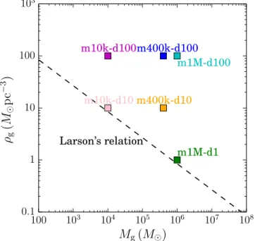
respectively). The initial conditions are summarized in Table1. Once we chose the cloud mass and density, the radius(Rg)
and the velocity dispersion in three dimensions (σg) are determined. Some of our models(such as models m1M-d1-s15, m1M-d1-s16, and m1M-d1-s17, with Mg=106Me and ρg=17 cm−3)roughly follow Larsonʼs relation(Larson1981):
L
1pc km s , 1
0.5 1
( ) ( )
s~⎛
-⎝
⎜ ⎞
⎠ ⎟
whereσis the velocity dispersion, andLis the size of the cloud (Heyer & Brunt2004; Mac Low & Klessen2004).
In Figure1we present the distribution of mass and density for the simulations listed in Table1. In order to determine the mass of a molecular cloud that is consistent with Larsonʼs relation, we adopt a velocity dispersion of sg GM Rg g. Some models initially have a higher velocity dispersion, which we motivate through cloud–cloud collisions (Furukawa et al.2009; Fukui et al.2013,2014)or to simulate molecular clouds in starburst galaxies. We further motivate and discuss our choice of the initial conditions in Section4.
2.2.2. SPH Simulations
We perform hydrodynamical simulations using the SPH codeFi(Hernquist & Katz1989; Gerritsen & Icke1997; Pelupessy et al. 2004; Pelupessy 2005) in the AMUSE framework. Our calculations have a relatively low mass resolution of m=1Me per particle. The gravitational soft-ening length during the hydrodynamical simulations is 0.1 pc, and the SPH softening length (h) is chosen such that
ρgh3=mNnb (Springel & Hernquist2002). HereNnb=64 is
instability down toh∼0.4 pc, which is smaller than the typical size of known embedded clusters (1 pc) (Lada & Lada2003) but somewhat larger than the observed typical width of gas filaments (∼0.1 pc) (Arzoumanian et al. 2011). With these limitations, we obviously cannot resolve the formation of individual stars, but we do resolve dense gas clumps. We think that the limited resolution of our hydrodynamical simulations does not pose a serious problem because we are interested in the global dynamical structure of the molecular cloud after only about an initial free-fall timescale,tff,i(see Table1for the
free-fall timescales for each of the initial models). In fact, after 0.9tff,i we stop the hydrodynamical simulation to analyze the
resulting gas distribution, initialize stars, and continue the simulations using a gravitational N-body code.
2.3. Star Formation
After stopping the hydrodynamical simulation (around
t
0.9ff, i
~ ), we replace some of the SPH particles with stellar particles. The selection of SPH particles is based, through the local gas densityρ, on the local SFEòloc:
M
100 pc . 2
loc sfe 3
0.5
( )
=a r -
⎛ ⎝
⎜ ⎞
⎠ ⎟
Hereαsfeis a free parameter in our simulations to control the SFE. The form of òloc (Equation (2)) is motivated by the
observations of individual molecular clouds for which the star-formation rate is argued to scale with the local free-fall timescale(Krumholz et al.2012; Federrath 2013b).
Here we adoptαsfe=0.02, which reproduces the observed global SFE across an entire molecular cloud of several percent, but also leads to a 10%–30% SFE in dense regions (>1000Mecm−3) (Lada & Lada 2003; Higuchi et al. 2009; Federrath & Klessen2013). In Table2 we present the global SFE (ò) and the SFE for the dense regions (òd) in our
simulations.
Depending on the local SFE, we replace individual gas particles with individual stellar particles, conserving their positions and velocities. For each selected particle, we assign a mass from the Salpeter mass function(Salpeter1955)between 0.3Me and 100Me, irrespective of the mass of its parent SPH particle. The mean mass of the adopted mass function is 1Me, which corresponds to the mass of individual SPH particles. Mass in our simulations is therefore globally conserved, but not locally.
2.4.N-body Simulations
After the stellar particles are initialized(mass randomly from the Salpeter mass function, and position and velocity from the parent SPH particle), we remove the residual gas, leaving only the stellar particles in the simulations. The instantaneous removal of the gas does not have a dramatic effect on the stellar distribution because most stars are formed in the densest regions where little low-density (residual) gas is present. The Table 1
Initial Conditions for the Hydrodynamical Simulations
Model Mass Radius Density Velocity Dispersion Initial Free-fall Time
Mg(Me) rg(pc) ρg(cm− 3
) σg(km s− 1
) tff, i(Myr)
m1M-d100-s7 1×10⁶ 13.4 1.7×10³ 19.6 0.81
m1M-d1-s15 1×10⁶ 62 17 9.1 8.1
m1M-d1-s16 1×10⁶ 62 17 9.1 8.1
m1M-d1-s17 1×10⁶ 62 17 9.1 8.1
m400k-d100-s1 4×10⁵ 10 1.7×10³ 14.4 0.82
m400k-d100-s2 4×10⁵ 10 1.7×10³ 14.4 0.82
m400k-d100-s3 4×10⁵ 10 1.7×10³ 14.4 0.82
m400k-d10-s8 4×10⁵ 21 170 9.9 2.5
m400k-d10-s9 4×10⁵ 21 170 9.9 2.5
m10k-d100-s4 1×10⁴ 2.87 1.7×10³ 4.2 0.81
m10k-d100-s5 1×10⁴ 2.87 1.7×10³ 4.2 0.81
m10k-d100-s6 1×10⁴ 2.87 1.7×10³ 4.2 0.81
m10k-d10-s11 1×10⁴ 6.2 170 2.9 2.6
m10k-d10-s12 1×10⁴ 6.2 170 2.9 2.6
m10k-d10-s13 1×10⁴ 6.2 170 2.9 2.6
Note.All models are supervirial, with∣Ek∣ ∣Ep∣=1.Here,“s”indicates the random seeds for the turbulence.
gas that is insufficiently dense to form stars tends to envelop the densest stellar conglomerates.
We now switch on theN-body code, for which we adopted the direct sixth-order Hermite predictor-corrector scheme (Nitadori & Makino 2008) without gravitational softening and with an accuracy parameter of η=0.1–0.25. The total energy error over the time span of the N-body simulations remained below ∼10−3.
The sizes of the stars we adopted from the zero-age main sequence radii for solar metallicity stars (Hurley et al.2000). We allow stars to collide using the sticky sphere approach. New stellar radii are assumed to be the zero-age main sequence radii for the new mass. Stellar mass loss was incorporated only at the end of the main sequence(Hurley et al.2000; see Fujii et al.2009; Fujii & Portegies Zwart 2013, for the details).
We did not perform the N-body simulations for models m10k-d10 (Mg=104Me and ρg=10Mepc−3=170 cm−3)
because the hydrodynamical simulations resulted in less than 100 stars, and we aim to have100Mestar clusters. In these simulations even the densest regions were<1000Mepc−3.
3. RESULTS
3.1. Formation of Embedded, Classical Open, and Young Massive Clusters
The N-body simulations are started at what we will call t=0 Myr. The initial distribution of stars follows the distribution of the densest regions in the turbulent molecular cloud. In Figure 2 we present a time series of snapshots of model m400k-d100-s3. The entire system continuously expands because not all stars are bound after gas expulsion. The distribution of stars is clumpy, and it takes a few Myr before the stars assemble into a more coherent aggregate.
We interrupt the simulations twice, at t=2 and at t=10 Myr, in order to analyze the stellar distribution and detect clustered aggregates. Clumps are found in these
snapshots by means of HOP (Eisenstein & Hut 1998) in AMUSE using an outer cutoff density of out 4.5Ms 4 Rh
3
( )
r = p
(three times the half-mass density of the entire stellar system,
M 8 R
h s ( h3)
r = p , where Ms is the total stellar mass and Rhis
the half-mass–radius relation of the entire distribution of the stars), a saddle-point density threshold (ρsaddle=8ρout), and the peak density threshold(ρpeak=10ρout), and the number of particles for the neighbor search (Ndense) and the number of
particles to calculate the local density(Nhop)are set to be 64.
The number of neighbors is used to determine which two groups merge, Nmerge=4. With these settings, the detection
limit of the clump mass is∼100Me. SometimesHOPidentifies multiple clumps as one, but by applying the method repeatedly we can separate those again. For this iterative procedure we adopt ρout=ρh,c, where ρh,c is the half-mass density of a detected clump. We continue this procedure untilρh,c100ρh, after which the clumps are so dense compared to the background that they do not separate anymore into substruc-tures(see Fujii2015bfor the details).
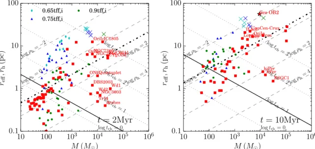
In Figure3we present the mass and half-mass radius of the star clusters obtained from our simulations at t=2 and at t=10 Myr. For comparison, we added a number of observed open clusters(classical open, embedded, young massive, and leaky clusters) to the same diagram. The majority of the identified clusters have masses and radii consistent with those of classical open clusters (Piskunov et al. 2008) (see also Fujii 2015b) and of known embedded clusters (Lada & Lada 2003). The densest initial molecular clouds ( m1M-d100, m400k-m1M-d100, and m400k-d10) tend to form massive compact clusters, similar to young massive clusters. Such compact clusters do not form in the less-dense or less-massive molecular clouds(such as m1M-d1 or m10k-d100).
When observing the 10-Myr-old stellar conglomerates from a distance, they tend to blend into a single star-forming region with an average density of∼0.01Mepc−3, which is compar-able to the mean field density in the solar neighborhood Table 2
Models forN-body Simulations
Model Mass Nof Particles Virial Ratioa SFE(Global) SFE(Dense)
Ms(Me) Ns ∣Ek∣ ∣Ep∣ ò òd
m1M-d100-s7 1.1×10⁵ 109080 0.9 0.11 0.27
m1M-d1-s16 1.9×10⁴ 18760 0.50 0.019 0.63
m1M-d1-s16-t0.75 4.6×10³ 4566 19 0.0046 0.42
m1M-d1-s16-t0.65 3.9×10³ 3855 131 0.0039 0.083
m1M-d1-s15-t0.75 5.9×10³ 5902 1.6 0.0059 0.49
m1M-d1-s15-t0.65 4.0×10³ 3954 80 0.0040 0.12
m1M-d1-s17-t0.75 5.5×10³ 5506 6.4 0.0055 0.26
m1M-d1-s17-t0.65 4.3×10³ 4322 63 0.0043 0.088
m400k-d100-s1 3.2×10⁴ 31895 1.3 0.078 0.22
m400k-d100-s2 2.3×10⁴ 23273 4.2 0.057 0.16
m400k-d100-s3 4.3×10⁴ 42596 0.43 0.096 0.25
m400k-d10-s8 1.5×10⁴ 14978 1.4 0.037 0.38
m400k-d10-s9 2.8×10⁴ 27891 0.41 0.068 0.39
m10k-d100-s4 4.1×10² 406 5.9 0.042 0.11
m10k-d100-s5 2.6×10² 256 7.4 0.027 0.079
m10k-d100-s6 2.5×10² 246 8.4 0.026 0.078
m10k-d10-s11 49 49 L 0.0049 0.00
m10k-d10-s12 61 61 L 0.0061 0.00
m10k-d10-s13 65 65 L 0.0065 0.00
Notes.Here,“s”indicates the random seeds for the turbulence.
a
Ek
∣ ∣and∣Ep∣are the total kinetic and potential energies of the entire stellar system, respectively. For virialized systems, the virial ratio equals 0.5. For models
Figure 2.Snapshots of model m400k-d100-s3. The size of the white dots indicates the masses of the stars: 8<m/Me<16 for the small dots, 16<m/Me<40 for middle sized, andm>40Mefor the largest dots. Stars with a massm<8Meare plotted as small blue dots.
(Holmberg & Flynn 2000). Such conglomerates may remain unrecognizable as a cluster system. For those simulations in which no clumps are detected down to a limit of 100Me, we adopt the median distance of the stars from the cluster center. The masses and half-mass radii of the clusters in our simulations mainly resemble the populations of observed embedded and classical open clusters. This result appears to be independent of the initial molecular-cloud density. Embedded and classical open clusters cluster around the point where the cluster age(tage)equals the dynamical time(tdyn)and
the half-mass relaxation time (trh) (see also Fujii2015b).
Here the dynamical time and the half-mass relaxation time are written as
t M
M
r
2 10
10 1 pc year 3
dyn 4 6
1 2 h
3 2
( )
~ ´
-
⎛ ⎝
⎜ ⎞⎠⎟ ⎛⎝⎜ ⎞⎠⎟
and
t M
M
r
2 10
10 1 pc year, 4
rh 8 6
1 2 h
3 2
( )
~ ´
⎛ ⎝
⎜ ⎞
⎠
⎟ ⎛
⎝
⎜ ⎞
⎠ ⎟
respectively (Portegies Zwart et al. 2010), where M is the cluster mass, and rh is the half-mass radius. For clarity we
assumed that the virial radius of star clusters is comparable to the half-mass radius and that the mean stellar mass is 1Me(as is the case in our simulations). In Figure3we present lines on which the relaxation (black full) and dynamical (black dash-dotted)times are equal to the age of the clusters, respectively. Both lines, as well as all the symbols, move upward with time. For the formation of young massive clusters, wefind that a dense, massive molecular cloud is necessary. The densities required to form such massive clusters exceed the density expected by Larsonʼs relation; the velocity dispersion neces-sary for the formation of young massive clusters is too high. Such an initial high density may be realized by cloud–cloud collisions (Fukui et al.2014). The velocity dispersion of our dense model is∼20 km s−1, which is comparable to the typical relative velocity of molecular clouds associated with young massive clusters, such as NGC 3603 and Westerlund 2. For these clusters, a collision between two molecular clouds was considered to trigger their formation (Furukawa et al. 2009; Ohama et al. 2010; Fukui et al. 2013, 2014), which is consistent with our findings here.
To form a star cluster in our simulations, the molecular cloud must be compressive(a high velocity dispersion due to a high density), which is consistent with observations (Zinnecker & Yorke2007). From various initial conditions, wefind that star clusters similar to open, known embedded, and young massive clusters form in these simulations, but leaky clusters (M∼104Meandrh∼10 pc)must form from different initial
conditions. We discuss the formation of leaky clusters in the following section (Section3.2).
3.2. Formation of Leaky Clusters
In the previous section, we show that known embedded, classical open, and young massive clusters form from turbulent molecular clouds, but no leaky cluster is found in our simulations. In this section we address the questions, How do leaky clusters form? Is the formation process different from the other clusters?
Pfalzner (2011) proposed that observed embedded clusters grow in mass and size due to star formation and become leaky clusters as a result of the expulsion of the residual gas. This scenario was later explored, and the evolutionary tracks of such a cluster on the mass–radius diagram were suggested (Parmentier & Pfalzner 2013; Pfalzner & Kaczmarek 2013; Pfalzner et al. 2014). Portegies Zwart et al.(2010), however, classified the leaky clusters as OB associations. Here we do not discuss if the leaky clusters are associations or clusters; we treat both leaky clusters and associations as less-dense clustered systems.
We consider leaky clusters (and also OB associations) to form clumpy distributions but that they lose this structure in the early dynamical evolution, contrary to the arguments in Pfalzner(2011). We support our argument with the simulation model m1M-d1-s16 (see the left panels in Figure 4). This simulation started with a spherical molecular cloud that collapsed asymmetrically because of the turbulent velocity field. Stars that formed mainly in the densest regions result in the stellar distribution being elongated and clumpy.
After the residual gas has been removed, the clusters tend to be supervirial, and some stars escape right away(see the virial ratio given in Table 2). As a consequence, the entire stellar distribution expands with time. At an age of t=10 Myr the density of the environment has decreased substantially, and the spatial distribution of the stars resembles leaky clusters and OB associations. In Figure5we present the spatial distribution of O and B spectral-type stars in the association Scorpius OB2(Sco OB2), which can be compared with our simulations in Figure4. Sco OB2 is composed of three subgroups: Upper Scorpius (USco), Upper Centaurus-Lupus(Upper Cen-Lup), and Lower Centaurus-Crux(Lower Cen-Crux) (Wolff et al.2007). These subgroups are listed in Pfalzner(2009)as leaky clusters and as associations in Portegies Zwart et al. (2010). They are all located at similar distances from the Sun, at 145 pc, 142, and 118 pc, respectively(Wolff et al.2007), and therefore they are considered to be a system. The distribution of massive(O and B) stars in Sco OB2 is very similar to the distribution of massive stars in model m1M-d1-s16 at an age of 10 Myr.
In Figure 6 we present the result of our clump-finding analysis for model m1M-d1-s16 at 2 Myr and at 10 Myr. At t=2 Myr we detected ∼20 clusters that are similar to observed embedded star clusters. At t=10 Myr no clear massive clusters remain visible in the snapshot(see Figure4), although we still detect several classic open cluster-like structures; in the epoch between 2 and 10 Myr, the stellar distribution has dispersed.
When interpreting the entire system in each simulation as a single association, the mass and radius are very similar to those of observed leaky clusters and OB associations. In Figure6we present these as crosses (near the top of the panels at 2 and 10 Myr). Model m1M-d1-s16 has an appearance and dynamical structure similar to the Sco OB2 system, rather than to the individual subclusters USco, Upper Lups, and Lower Cen-Crux. In this analysis we excluded single stars (those with a local densityρ6<10−3Mepc−3), which is more than an order of magnitude lower than the mean density of the solar neighborhood (ρ6 here is the density measure within the six nearest neighbors).
hydrodynamical simulations(at∼0.9tff,i). In the observed
star-forming regions, however, stars appear to form when the local density exceeds some threshold density for self-gravitating clouds of∼103cm−3(McKee & Ostriker2007), and feedback starts to dominate the hydrodynamics as soon as the first massive star forms, which may happen well before a free-fall timescale. The free-fall timescale of model m1M-d1-s16 is
∼8 Myr, which is considerably longer than the formation time for massive stars(∼1 Myr) (McKee & Ostriker2007). In such a region, where the star-forming timescale is considerably smaller than the free-fall timescale of the entire molecular cloud, stellar feedback is expected to terminate the star formation before the molecular cloud fully collapses. This would result in a less-clumpy stellar distribution.
Unfortunately, in our simulations, we cannot take such gradual star formation and feedback processes into account, although they have been addressed with the AMUSE frame-work by Pelupessy & Portegies Zwart (2012). In order to mimic the early star-formation process, we experimented with stopping the hydrodynamical simulations at an earlier epoch and replacing the gas particles with stellar particles.
As in our previous simulations, we assumed that the feedback terminates star formation and causes the residual gas to be ejected instantaneously. We stop the hydrodynamical Figure 4.Snapshots att=2(top)and 10(bottom)Myr for model d1-1M, but for different timing of gas removal:t=0.9, 0.75, and 0.65tff,i(models m1M-d1-s16,
m1M-d1-s16-t0.75, and m1M-d1-s16-t0.65, respectively)from left to right.
simulation for model m1M-d1-s16 att=0.65tff,iand 0.75tff,i
(5.3 and 6.2 Myr, respectively) and replace gas particles with stellar particles in the same way as for model m1M-d1-s16, i.e., assuming a local SFE given by Equation (2) and the same values for αsfe=0.02. The numbers of stars that form using this procedure decrease considerably, and the resulting virial ratio of the stellar system increases. We also run the same initial conditions but with different random seeds(m1M-d1-s15 and m1M-d1-s17). In Table 2 we present some global parameters for these models.
Snapshots of these models (d1-s16-t0.75 and m1M-d1-s16-t0.65) are shown in the middle and right panels of Figure4. The distribution of massive stars is less clumpy than that of model m1M-d1-s16 (standard model, in which the hydrodynamical simulation is stopped at 0.9tff; see the left
panels of Figure4). We also apply the clump-finding algorithm to these models, the results of which are shown in Figure6. At t=2 Myr, several clumps are detected in both models, but they are less dense than those detected in our standard model. In model m1M-d1-s16-t0.65 in particular, the density of the detected clumps is only slightly elevated compared to the background density in the solar neighborhood (0.01Mepc−3) (Holmberg & Flynn2000), and these clumps may therefore not be recognized as clusters. In model m1M-d1-s16-t0.75 some clumps that resemble open clusters are still detected at t=10 Myr, but none in model m1M-d1-s16-t0.65. If we treat the entire system as one cluster, the masses are similar to those of leaky clusters and associations, even though the size remains larger by about a factor of two. In Figure6we present the mass and half-mass radius of the resulting clusters for stars with
ρ6>10−3Mepc−3.
Our assumption that star formation terminates instanta-neously throughout the system after about one free-fall time of the molecular cloud probably overestimates the effect of the feedback considerably. In observed star-forming regions, the feedback from massive stars tends to limit star formation locally, but it may not affect the entire (∼100 pc across) star-forming region. In the simulations of Pelupessy & Portegies
Zwart (2012), the wind of one massive ∼30Me star blows the residual gas from the clustered environment in a couple of Myr, which is much longer than that adopted in our simulations.
If star formation proceeds as clumpy as simulated here, the feedback is even more localized, which will result in a considerable age spread among subgroups. Our simulations would then be representative for the formation of cluster complexes such as USco, Upper Lups, and Lower Cen-Crux, or OB associations such as Sco OB2. The ages of these three subgroups are slightly different from each other: 14–15, 11–12, and 5–6 Myr for Upper Cen-Lup, Lower Cen-Crux, and USco, respectively (Wolff et al. 2007). If we could assume local feedback processes, an association (or leaky clusters) similar to Sco OB2 might form from an initial condition, such as models m1M-d1. Less-dense clusters tend to have wider age spreads(Parmentier et al.2014), which is also consistent with our simulations. We therefore argue that the ancestors of associations are conglomerates of denser embedded clusters. We detect these as an environment with multiple low-mass but rather dense clusters that disperse in time. The evaporation of these clusters is driven by relaxation and feedback, and this makes them resemble associations.
4. INITIAL CONDITIONS OF MOLECULAR CLOUDS
In the previous section, we showed that our dense models tend to form young massive clusters and that less-dense models lead to leaky clusters as well as known embedded and classical open clusters. The type of the resulting star clusters is sensitive to the initial conditions of the parental molecular clouds. In this section, we compare our initial conditions with observed molecular clouds and discuss a model for the formation of clusters in the Milky Way and other nearby galaxies.
relation. In order to estimate the mass of molecular clouds following Larsonʼs relation, we assume that the molecular clouds are in virial equilibrium(i.e., they satisfysg2=GM rg g, where σg, Mg, and rg are the velocity dispersion, mass, and
radius of the molecular clouds, respectively). Observed molecular clouds, however, are not necessarily virialized.
Molecular clouds in the Milky Way tend to follow Larsonʼs relation, but with a large scatter of the density. On the other hand, not all of our initial conditions are consistent with the mass and density of molecular clouds observed in the Milky Way. Models m10k-d100(104Meand 100Mepc−3; 1700 cm−3) and m10k-d10 (104Me and 10Mepc−3; 170 cm−3), for example, are initially indistinguishable from typical molecular clouds in the Milky Way.
As we described in Section3, the number of stars formed in model m10k-d10 was too small (fewer than 100 stars) to be recognized as a cluster in our analysis. Model m10k-d100 produces a sufficiently large number of stars but does not form a recognizable cluster after 2 Myr. If we treat the entire region of this model as a cluster conglomerate, the mass and radius are similar to that of an open cluster. From this, we conclude that the molecular clouds typical in the Milky Way tend to form classical open clusters, but that they are insufficiently massive and dense to form massive star clusters.
Model m1M-d1(106Meand 1Mepc−3)represents the most massive molecular cloud in the Milky Way(Murray2011), and it follows Larsonʼs relation. This initial condition results in several embedded cluster cores, which eventually evolve to a conglomerate of associations.
The initial conditions that tend to form young massive clusters are considerably denser than the molecular clouds observed in the Milky Way (see Figure 7). To form young massive clusters in our simulations, a mass of at least several
105Me and a mean density of 10Mepc−3 (170 cm−3) are required. Such initial conditions are common in local starburst galaxies, but very rare in the Milky Way.
In Figure 7 we present the estimated mass and density of molecular cloud density typical for local starburst and disk galaxies. These data are obtained from Krumholz et al.(2012). We calculated the masses and densities for these molecular clouds from the free-fall timescale provided by Krumholz et al. (2012)using the observed surface gas densities(Sg). Krumholz et al. (2012) considered two rather distinct regimes of molecular clouds: the molecular cloud regime and the Toomre regime. The molecular cloud regime is expected to be common in local disk galaxies. The molecular clouds are decoupled from their surrounding interstellar medium and as a result are self-gravitating(Krumholz et al.2012). The Toomre regime is common in starburst galaxies. In this case the interstellar medium is highly turbulent, and therefore the free-fall timescale of the molecular clouds should be estimated using the midplane pressure in the galactic disks(see Krumholz et al.2012, for the details).
Following the description of Krumholz et al. (2012), we estimate the typical mass of molecular clouds for each galaxy listed in Krumholz et al.(2012). We take the smaller free-fall timescale for the molecular cloud and Toomre regimes(tff,GMC
and tff,T, respectively) as the free-fall timescale(tff), which is
consistent with Krumholz et al. (2012). We calculate the density through the free-fall timescale using
Gt
3
32 . 5
g
ff2
( )
r = p
In the Toomre regime, the midplane pressure in the disk of surface gas densityΣgis
P G
2 . 6
P
g,T g 2
g 2
( )
r s f p
= = S
Hereρg,Tis the molecular cloud density in the Toomre regime,
σg is the velocity dispersion of the gas, and fP is a dimensionless factor (Krumholz et al. 2012). The Toomre Q for the gas is written as
Q
G
2 1
. 7
g
g
( )
( )
b s
p
= + W
S
Hereβis the logarithmic index of the rotation curve(β=0 for aflat rotation curve, whereas for solid-body rotation β=1), and Ω=2π/torb (torb is the galactic orbital period) is the
angular velocity of galactic rotation (see also Krumholz & McKee 2005). From these equations, the density of the molecular cloud becomes
GQ
1
. 8
P
g, T
2
2
( )
( )
r b f
p
+ W
Here we adopt Q∼1 and β=0 following Krumholz et al. (2012). If we assume that the cloud is virialized—i.e.,
GM r
g 2
g,T g
s ~ , whereMg,T andrgare the mass and radius of
the cloud—from Equation(7)and g,T 3Mg,T 4 rg 3
( )
r = p , we can
estimate the cloud mass using
M 1 G t
32 3
. 9
g,T 3 2 g3 orb3 g
1 2
( )
p r
~ S
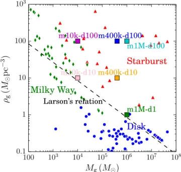
-Figure 7. Mass–density relation of observed molecular clouds. Green diamonds indicate individual molecular clouds in the Milky Way galaxy. Blue circles and red triangles are for molecular clouds typical in individual local disk and starburst galaxies, respectively. Each point indicates one galaxy. The data are from Krumholz et al.(2012). Color squares indicate our initial conditions, which are the same as those shown in Figure1. The dashed line indicates the mass–density relation following Larsonʼs relation for a virialized cloud( g2 GM R
g g
Because for each galaxy torb and Σg are given in Krumholz
et al.(2012), we can estimate the cloud density and mass from Equations (8) and (9). Here we adopt fP;3, following Krumholz et al.(2012).
For the molecular cloud regime (i.e., tff,GMC<tff,T), the
mass is estimated as follows. The mass of molecular clouds is estimated by the two-dimensional Jeans mass in galactic disks (Kim & Ostriker 2002; McKee & Ostriker 2007; Chandar et al.2011), which is given by
M
G , 10
g,GMC g 4
2 g
( )
s =
S
(see Equation(3) of Krumholz et al. 2012). Since the mass and density of molecular clouds in the molecular cloud regime are written as Mg,GMC=prg2 SGMC and rg,GMC=
M r
3 4 g,GMC g3
( p) - , where ΣGMC is the surface density of
molecular clouds, using Equation (10) we can calculate the density of molecular clouds with (Equation(4) in Krumholz et al.2012)
G
3
4 . 11
g,GMC
GMC 3
g
g
2 ( )
r p
s
= S S
Here we adoptΣGMC=85Mepc−2andσg=8 km s−1for all
galaxies following Krumholz et al. (2012). Using Equa-tions (10) to (11), we obtain the mass and density in the molecular cloud regime using the value forΣgfrom Krumholz
et al.(2012).
The obtained masses and densities for molecular clouds in the local disk and starburst galaxies are presented in Figure7. Most galaxies are in the Toomre regime (and only 13 disk galaxies are in the molecular cloud regime). The molecular clouds typical for starburst galaxies are factors of 10–100 denser than those following Larsonʼs relation. Our massive and dense models (m400k-d100, m400k-d10, and m1M-d100), which form young massive clusters, are consistent with the molecular cloud observed in starburst galaxies. Starburst galaxies such as M83(Bastian et al.2011)and M51(Chandar et al.2011)are indeed rich in dense, massive clusters. On the other hand, molecular clouds typical in local disk galaxies do follow Larsonʼs relation. Our model m1M-d1, which forms classical open and leaky clusters (associations), appears to be quite similar to these molecular clouds.
The typical molecular cloud in a disk galaxy, such as the Milky Way, tends to form classical open clusters and associations, but these clouds are insufficiently massive to form young massive star clusters. This is consistent with the abundance of open star clusters and associations in the Milky Way and with the lack of massive star clusters. According to our simulations, the formation of a massive star cluster requires a massive (∼105–106Me) and dense (∼10–100Mepc−3) molecular cloud. Such a massive molecular cloud has, if virialized, a velocity dispersion of ∼20 km s−1. Such a high velocity dispersion(under compressive conditions)could result from the collision between two clouds (Furukawa et al.2009; Ohama et al. 2010; Fukui et al. 2014). Comparable high velocities are observed in the regions surrounding young massive clusters, such as in the vicinity of NGC 3603(Fukui et al. 2014)and Westerlund 2 (Furukawa et al. 2009; Ohama et al.2010). These clusters are claimed to have been the result
of cloud–cloud collisions (Furukawa et al. 2009; Ohama et al.2010; Fukui et al.2014). These claims are supported by three-dimensional magnetohydrodynamic simulations, which also suggest that such cloud–cloud collisions initiate the formation of massive cloud cores and potentially form massive star clusters(Inoue & Fukui2013).
Although our initial conditions of molecular clouds cover a relatively wide range of mass and density, they are limited by our choice to opt for homogeneous-density spheres. Recent numerical studies indicate that molecular clouds with a concentrated density profile such as a power law tend to form one high-mass star in the center surrounded by many low-mass stars(Girichidis et al.2011,2012). Such centrally concentrated models then may more efficiently lead to the formation of massive clusters than our adopted homogeneous initial conditions.
5. MASS AND RADIUS EVOLUTION OF YOUNG STAR CLUSTERS
Star clusters can be subdivided into several types, which represent themselves clearly when presented in a mass–radius diagram. The mass–radius distribution of star clusters changes with time. Here we discuss the time evolution of the mass and radius of young clusters.
5.1. Observations
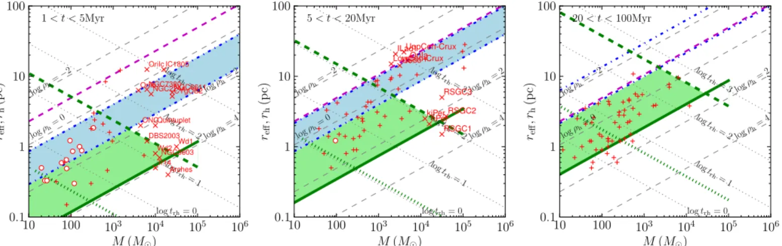
We start with summarizing the mass and radius evolution of observed young star clusters. These observations are presented in Figure 8, in particular for observed embedded clusters, classical open star clusters, young massive(starburst)clusters, and associations(Hodapp & Rayner 1991; Drew et al. 1997; Horner et al. 1997; Lada & Lada2003; Luhman et al. 2003; Andersen et al. 2006; Levine et al. 2006; Flaherty & Muzerolle 2008; Piskunov et al. 2008; Fang et al. 2009; Pfalzner2009; Winston et al.2009; Portegies Zwart et al.2010; Bonatto & Bica2011). For clarity we bin the clusters in age in intervals oftage=1–5 Myr, 5–20 Myr, and 20–100 Myr.
Pfalzner(2009)and Portegies Zwart et al.(2010)list several young massive clusters, but in many cases the listed radii differ. We adopt the half-mass radius given in Portegies Zwart et al. (2010) because the radius presented in Pfalzner (2009) corresponds to the core radius of the clusters rather than the half-mass radius. The former gives a more direct comparison with our simulations. In our analysis we try to stay as much as possible to the same definition of cluster radius. Piskunov et al. (2008) present projected core and tidal radii by fitting King models(King1966). Because the density profiles for the open clusters listed in Piskunov et al. (2008)are very shallow, we adopted their core radii, which for a King model withW0=3
is quite similar to the half-mass radius (the ratio of the three-dimensional core radius to half-mass radius is 0.65 for a King model withW0=3).
region of the left and middle panels (t=1–5 Myr and 5–20 Myr, respectively), and young massive clusters are found to the right in the diagrams in Figure 8. As was already suggested by Pfalzner (2009), young massive star clusters are well separated in mass and radius from embedded and open clusters. This separation, however, diminishes for the older age group(20–100 Myr; see the right panel of Figure8).
5.2. Analytical Model for the Dynamical Evolution of Young Star Clusters
The distribution and evolution of the observed star clusters in mass and radius can be understood from our models of the dynamical evolution for star clusters.
The lower limit of the cluster density can be understood by considering the background density in the field. The magenta dashed line in the diagram indicatesρ=0.1Mepc−3, which is an order of magnitude higher than the mean density of thefield stars in the solar neighborhood(Holmberg & Flynn2000). We adoptρ=0.1Mepc−3as a lower limit for the cluster density (magenta dashed line in Figure8). Star clusters with a density similar to or lower than the mean stellar density would therefore not be recognizable as clusters. And indeed, only a few of the most massive clusters reside above this curve, and those have a relatively high concentration. As a consequence, their core densities exceed the local density considerably, which helps to identify them as clusters in observational campaigns.
The blue dash-dotted lines in Figure 8 indicate the mass– radius relation for which the dynamical timescale (see Equation (3)) is equal to the age of the cluster. Each panel contains two lines, one for the minimum and one for the maximum age of the clusters shown in the panels. The region between these lines is shaded blue. Clusters between or below the blue lines will be recognizable as bound systems unless the lines exceed the magenta dashed line. Portegies Zwart et al. (2010) and Gieles & Portegies Zwart (2011) argued that the ratio between cluster age and dynamical time provides a good indicator for separating the bound from the unbound systems: they adopt as a criteriontage tdyn3to make this distinction. Using this criterion, they categorized the leaky clusters in Pfalzner (2009) as associations. The blue region in Figure 8
moves upward with time, together with the observed clusters. Att>20 Myr (the right panel in Figure8)the blue lines are located above the magenta line, indicating that these clusters have a density too low to be recognized as clusters.
The evolution of dense star clusters is quite different from those of open clusters or associations. Dense star cluster evolution can roughly be divided into two phases: before core collapse and after core collapse. In the former phase, the core radius of the star clusters shrinks, and as a consequence its core density increases (Hénon1965; Lynden-Bell & Wood 1968). From the moment thefirst hard binaries form in the cluster core (Spitzer & Hart 1971; Aarseth 1974), they act as energy sources (Heggie 1975; Hut 1983), causing the core to re-expand. From this moment on, the core- and half-mass radii of clusters increases. These processes proceed on the half-mass relaxation time:
t
G m
0.065
ln . 12
rh
3
2 ( )
s r =
á ñ L
Here σ and ρ are the velocity dispersion and density of the cluster, respectively, and lnL is the Coulomb logarithm (Spitzer 1987). We rewrite Equation (12) to include some common dimensions in Equation(4).
Gieles et al. (2011) modeled the postcollapse evolution of the half-mass radius and density of star clusters due to the energyflux from the core, following the description of Hénon (1965). We attempt to understand the dynamical evolution of young star clusters using their description. We ignore the precollapse phase and consider only the evolution in the postcollapse (expansion)phase because the precollapse phase is much shorter than the postcollapse. The core-collapse time, which is the time for the precollapse phase, scales with the relaxation time (see Equation (4) or (12)). This timescale depends on the stellar mass function, and for clusters with a realistic mass function the core-collapse time is generally shorter than one relaxation(Portegies Zwart & McMillan2002; Gürkan et al.2004; Fujii & Portegies Zwart2014). Since most of the young open clusters in our observed sample have a relaxation time10 Myr(see the left panel of Figure8), they probably reach core collapse well within a few Myr. We also ignore the effect of the Galactic tidalfield because the timescale Figure 8.Mass–radius diagrams of observed young star clusters fortage=1–5, 5–20, and 20–100 Myr from left to right. The data are from Lada & Lada(2003)for
we treat here is short(<100 Myr)compared to the timescale for the tidal disruption (∼1 Gyr) (Gieles et al.2007).
The time of the half-mass radius of clusters due to binary heating in the core is given by Equation (B7) in Gieles et al. (2011):
r G
N t
3
4 125 . 13
h
1 3
2 3
( ) ( )
p z
⎜⎛ ⎟
⎝ ⎞ ⎠
HereNis the initial number of stars in the cluster. In Equation (B7) in Gieles et al. (2011), the cluster mass is assumed as
M= á ñm N, whereá ñm is the mean stellar mass. They adopted a scaled mass ofá ñ =m 0.5, and as a result their Equation(B7) is slightly different from our equation. If we assume that
m 0.5M
á ñ = , we can write this equation as
r M
M
t
2.0
Myr pc. 14
h 2 3
1 3 age
2 3
( )
z
-
⎛ ⎝
⎜ ⎞⎠⎟ ⎛⎝⎜ ⎞⎠⎟
Here we adopt t=tage because we ignore the precollapse
phase. The expansion-rate coefficient,ζ, depends on the ratio of the maximum to the minimum mass in the stellar mass function, μ≡mmax/mmin. In Gieles et al. (2011) we use ζ;0.2, which corresponds to μ;10, and which is appro-priate for globular clusters. Young clusters, however, should have a larger value of μ because of the presence of massive stars. For some of these clusters, mmax/mmin;100Me/
0.01Me;104. Following Gieles et al. (2011) and assuming
ζ∝μ1/2, we obtainζ;20 for μ;104. Equation (14) with ζ=20 fort=tage=2, 10, 40 Myr is shown as green dashed
lines in Figure8.
The majority of the observed clusters are located below this evolutionary line rather than straddling the line, which indicates that they haveζ<20. The green dotted lines in each panel of Figure 8 show Equation (14) with ζ=0.2. Most of the observed embedded and classical open clusters are located between the dotted green (for ζ=0.2) and the dashed green (ζ=20)lines. This may be caused by the large dispersion inζ, as we discussed here, or because the precollapse time is not taken into account in our analysis. By ignoring the precollapse time we reduce the evolution time of a star cluster compared to the expectation.
The descriptions of Gieles et al.(2011) (Equations(13)and (14)) give infinite density at t=0 Myr, which hardly seems realistic for actual young star clusters. Instead, we adopt Equation(B4)of Gieles et al.(2011):
G N
t
1
250 , 15
h
2
( )
r
z
⎛
⎝
⎜ ⎞
⎠ ⎟
which gives the half-mass density as a function of time. We also adoptá ñ =m 0.5M. We assume a(maximum)half-mass
density of 104Mepc−3 at tage=0.1 Myr irrespective of the
cluster mass; we obtain rh(Mpc-3)=100(t Myr)-2. Since
M r
3 8
h ( h3)
r = p , the relation can be written as
r M
M
t
0.0158
Myr pc . 16
h
1 3 age
2 3
( ) ( )
=
⎛ ⎝
⎜ ⎞⎠⎟ ⎛⎝⎜ ⎞⎠⎟
Equation(16)is presented in Figure8as the solid green line. One naively expects that clusters with an initial density smaller than 104Mepc−3populate the area above this line, which is
consistent with the observations. From a theoretical perspective we argue that star clusters are expected to reside in the green and blue regions in Figure 8, which for the majority of observed clusters appears to be the case.
From these results, the regions in which clusters are expected to exist on mass–radius diagrams are shown by the green and blue shades in Figure8, and the observed distribution of star clusters matches them. Furthermore, our analytical models suggest two distinct populations of massive(~104M
)clusters,
which are called starbursts and leaky clusters by Pfalzner (2009). We argue that these two populations naturally appear if we consider the formation and the dynamical evolution process of star clusters.
5.3. Time Evolution of Cluster Radius: Leaky and Starburst Clusters
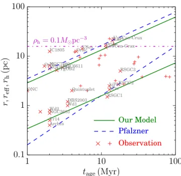
Young star clusters withM∼104Meare divided into two groups, as can be seen in Figure8. Pfalzner(2009)named them starburst(young massive)clusters and leaky clusters(following Portegies Zwart et al. 2010we identify the latter category as associations). Pfalzner (2009, 2011) showed that both families of clusters expand with time, but at a different rate: r/pc=0.16(tage/Myr) for the starburst clusters and r pc=3.5(tage Myr)2 3 for the associations. In this section, we discuss the origin of these different evolutionary tracks.
In Figure9we present the age and radius of observed young star clusters with a mass of 103<M<105Me. The time evolution for cluster radii, plotted as the solid green lines, is obtained from the analytic models discussed in Section5.2.
Associations are about one dynamical timescale old, and therefore we can hardly confirm whether they are bound or not. If we consider them to be one dynamical timescale old, i.e., Figure 9.Cluster radius as a function of time for clusters with a mass of 103– 105Me. Red cross signs are from Portegies Zwart et al.(2010)and red pluses from the others(see the caption of Figure8). Blue dashed lines are the relations given in Pfalzner (2009, 2011): r=3.5tage2 3 and r=0.16tage for top and
bottom, respectively. Green lines are cluster radii as a function of time obtained from our model: rh=2.7tage2 3 and rh=0.34tage2 3 for top and bottom,
tagetdyn, Equation (3) gives rh pc=2.7(tage pc)2 3. We present this relation in Figure9as the top green line. The model is consistent with the observed clusters, and the power-law index of our model is consistent with that of Pfalzner(2011). For starburst clusters, we adopt the results based on Gieles et al. (2011). By adopting M=104Me in Equation(16), we obtainrh pc=0.34(tage Myr)2 3. We present this relation in Figure 9 as the bottom green line. In part due to the large scatter, this relation is also consistent with the observed radius evolution of starburst clusters.
The magenta dash-dotted line in Figure9 gives the relation
ρh=0.1Mepc−3. This is an order of magnitude higher than the field density in the solar neighborhood (0.01Mepc−3) (Holmberg & Flynn 2000), and we assume this to be a minimum to the(observable)cluster density. This predicts that associations will not survive more than ∼20 Myr, and indeed no such a cluster has been observed.
6. SUMMARY
We performed a series of simulations of star-forming regions. Our calculations start with hydrodynamical simula-tions of turbulent molecular clouds. These simulasimula-tions are continued for about one initial free-fall timescale, after which we replace gas particles with stars, adopting a local SFE (Krumholz et al. 2012). The stellar masses are selected randomly from the adopted initial mass function, and the stars receive the position and velocity of the gas particles they replace. We subsequently remove all residual gas and continue the evolution of the young emerging star cluster by means of N-body simulations with stellar evolution.
The types of star clusters that formed in our simulations depend on the initial conditions (mass and density) of the molecular cloud. The clouds with initial conditions typical for those observed in the Milky Way(104M
and 100–1000 cm−3)
lead to classical open clusters. More massive clouds (105– 106Me) with the same density evolve into dense, massive clusters. These massive molecular clouds are common in starburst galaxies, but are very rare in local disk galaxies such as the Milky Way. This result is consistent with observations that young massive clusters are common in starburst galaxies, but only several have been found in the Milky Way. We argue that such massive clouds must be able to form in the Milky Way Galaxy, even though they are probably rare.
Dense, massive clusters in our simulation form from molecular clouds with a mass of 106Me and a density of
∼1000 cm−3(100Mepc−3), leading to a velocity dispersion of
∼20 km s−1. This is consistent with the relative velocity of molecular clouds observed near young massive clusters in the Milky Way, such as near NGC 3603 (Fukui et al.2014)and Westerlund 2(Furukawa et al. 2009; Ohama et al.2010). We argue that massive clusters in the Milky Way can therefore not form from individual clouds, but their formation may have been initiated in cloud–cloud collisions(Furukawa et al.2009; Ohama et al.2010; Fukui et al.2014).
Molecular clouds with a mass of∼106Meand a low density of ∼10 cm−3 (∼1Mepc−3), which follow Larsonʼs relation, tend to form associations (“leaky clusters”in the terminology of Pfalzner 2009). These relatively low-density and massive molecular clouds form a number of small clumps. They might be detected as embedded or classical open clusters when they are young, but they evolve to less-dense clusters by gas
expulsion and relaxation. After several Myr, these systems lose their clumpiness and become recognizable as associations.
In our simulations, we assumed that stars form instanta-neously upon the expulsion of the residual gas(after an initial free-fall time of the molecular cloud). Our prescription for star formation is simple compared to reality, in which star formation triggers the expulsion of the residual gas by means of feedback processes. Regardless of the simplicity of our approach, we are still able to make a distinction between the formation of associations, open clusters, and massive star clusters.
The young stellar system, Sco OB2, is an assembly of associations of slightly different ages: USco, Upper Cen-Lups, and Lower Cen-Crux. A stellar system similar to Sco OB2 naturally originates in our simulations of relatively massive and low-density molecular clouds, although the age spread cannot be reproduced with our method. The relation that less-dense clusters have wider age spreads of stars is observationally and theoretically suggested(Parmentier et al.2014).
In addition, we compared our simulations with theoretical models for cluster expansion that are due to the dynamical evolution (Gieles et al. 2011). These models satisfactorily explain the evolution in radius of simulated clusters as well as of the observed clusters.
We also found that the distribution of clusters on the mass– radius diagram is also limited by the density with which the dynamical timescale is equal to the cluster age. This implies that, if the cluster age is much shorter than the dynamical time, such clusters cannot be recognized as(bound)systems(Gieles & Portegies Zwart2011). After;20 Myr the density of these associations drops below the background density, and they dissolve.
The gap of the radius distribution for associations and young massive clusters suggested by Pfalzner (2009) is consistent with our simulation results. Whereas young massive clusters evolve following the cluster expansion model, leaky clusters havetage∼tdyn. With our models, the evolution of radius for
observed leaky and young massive clusters are described by rh pc=2.7(tage pc)2 3 and rh pc=0.34(tage Myr)2 3, respectively. These are also consistent with observations. Pfalzner et al.(2014)claimed that star formation continues in embedded clusters and that after the gas expulsion they expand and become associations. Our models, however, indicate that clumpy star-forming regions are observed as a conglomerate of embedded clusters, but at a later time these systems lose their clumpiness through the expulsion of the residual gas and two-body relaxation. Because our coverage of parameter space remains limited and much is still to be uncovered, we hope to explore a much wider range of initial conditions of molecular clouds (different masses, radii, and density distributions) and other assumptions for star formation(different epochs for star formation and gradual gas removal rather than instantaneous gas expulsion).
Our results suggest that the difference in the parental molecular clouds results in the formation of various types of star clusters if we assume the same star-formation process and that the cluster-formation process does not depend on the condition of the galaxy, either normal disk or starburst.
Council NWO (grants #643.200.503, #639.073.803 and #614.061.608), and the Netherlands Research School for Astronomy (NOVA). Numerical computations were partially carried out on a Cray XC30 at the Center for Computational Astrophysics (CfCA) of the National Astronomical Observa-tory of Japan and the Little Green Machine at Leiden Observatory.
REFERENCES
Aarseth, S. J. 1974, A&A,35, 237
Andersen, M., Meyer, M. R., Oppenheimer, B., Dougados, C., & Carpenter, J. 2006,AJ,132, 2296
Arzoumanian, D., André, P., Didelon, P., et al. 2011,A&A,529, L6 Bastian, N., Adamo, A., Gieles, M., et al. 2011,MNRAS,417, L6 Bonatto, C., & Bica, E. 2011,MNRAS,414, 3769
Bonnell, I. A., Bate, M. R., & Vine, S. G. 2003,MNRAS,343, 413 Chandar, R., Whitmore, B. C., Calzetti, D., et al. 2011,ApJ,727, 88 Drew, J. E., Busfield, G., Hoare, M. G., et al. 1997,MNRAS,286, 538 Eisenstein, D. J., & Hut, P. 1998,ApJ,498, 137
Fang, M., van Boekel, R., Wang, W., et al. 2009,A&A,504, 461 Federrath, C. 2013a,MNRAS,436, 1245
Federrath, C. 2013b,MNRAS,436, 3167 Federrath, C., & Klessen, R. S. 2013,ApJ,763, 51
Federrath, C., Roman-Duval, J., Klessen, R. S., Schmidt, W., & Mac Low, M.-M. 2010,A&A,512, A81
Figuerêdo, E., Blum, R. D., Damineli, A., & Conti, P. S. 2002,AJ,124, 2739 Flaherty, K. M., & Muzerolle, J. 2008,AJ,135, 966
Fujii, M., Iwasawa, M., Funato, Y., & Makino, J. 2009,ApJ,695, 1421 Fujii, M. S. 2015a, PASJ,67, 59
Fujii, M. S. 2015b, PASJ, arXiv:1410.5540
Fujii, M. S., & Portegies Zwart, S. 2013,MNRAS,430, 1018 Fujii, M. S., & Portegies Zwart, S. 2014,MNRAS,439, 1003 Fujii, M. S., & Portegies Zwart, S. 2015,MNRAS,449, 726 Fukui, Y., Ohama, A., Hanaoka, N., et al. 2013, arXiv:1306.2090 Fukui, Y., Ohama, A., Hanaoka, N., et al. 2014,ApJ,780, 36 Furukawa, N., Dawson, J. R., Ohama, A., et al. 2009,ApJL,696, L115 Gerritsen, J. P. E., & Icke, V. 1997, A&A,325, 972
Gieles, M., Athanassoula, E., & Portegies Zwart, S. F. 2007, MNRAS, 376, 809
Gieles, M., Heggie, D. C., & Zhao, H. 2011,MNRAS,413, 2509 Gieles, M., & Portegies Zwart, S. F. 2011,MNRAS,410, L6
Girichidis, P., Federrath, C., Allison, R., Banerjee, R., & Klessen, R. S. 2012, MNRAS,420, 3264
Girichidis, P., Federrath, C., Banerjee, R., & Klessen, R. S. 2011,MNRAS, 413, 2741
Gürkan, M. A., Freitag, M., & Rasio, F. A. 2004,ApJ,604, 632 Heggie, D. C. 1975,MNRAS,173, 729
Hénon, M. 1965, AnAp,28, 62
Hernquist, L., & Katz, N. 1989,ApJS,70, 419
Heyer, M. H., & Brunt, C. M. 2004,ApJL,615, L45
Higuchi, A. E., Kurono, Y., Saito, M., & Kawabe, R. 2009,ApJ,705, 468 Hodapp, K.-W., & Rayner, J. 1991,AJ,102, 1108
Holmberg, J., & Flynn, C. 2000,MNRAS,313, 209 Horner, D. J., Lada, E. A., & Lada, C. J. 1997,AJ,113, 1788 Hurley, J. R., Pols, O. R., & Tout, C. A. 2000,MNRAS,315, 543 Hut, P. 1983,ApJL,272, L29
Inoue, T., & Fukui, Y. 2013,ApJL,774, L31 Kim, W.-T., & Ostriker, E. C. 2002,ApJ,570, 132 King, I. R. 1966,AJ,71, 64
Krumholz, M. R., Dekel, A., & McKee, C. F. 2012,ApJ,745, 69 Krumholz, M. R., & McKee, C. F. 2005,ApJ,630, 250 Lada, C. J., & Lada, E. A. 2003,ARA&A,41, 57 Larson, R. B. 1981,MNRAS,194, 809
Levine, J. L., Steinhauer, A., Elston, R. J., & Lada, E. A. 2006,ApJ,646, 1215
Luhman, K. L., Stauffer, J. R., Muench, A. A., et al. 2003,ApJ,593, 1093 Lynden-Bell, D., & Wood, R. 1968,MNRAS,138, 495
Mac Low, M.-M., & Klessen, R. S. 2004,RvMP,76, 125 McKee, C. F., & Ostriker, E. C. 2007,ARA&A,45, 565 Murray, N. 2011,ApJ,729, 133
Nitadori, K., & Makino, J. 2008,NewA,13, 498
Ohama, A., Dawson, J. R., Furukawa, N., et al. 2010,ApJ,709, 975 Ostriker, E. C., Stone, J. M., & Gammie, C. F. 2001,ApJ,546, 980 Parmentier, G., & Pfalzner, S. 2013,A&A,549, A132
Parmentier, G., Pfalzner, S., & Grebel, E. K. 2014,ApJ,791, 132 Pelupessy, F. I. 2005, PhD thesis, Leiden Observatory, Leiden Univ. Pelupessy, F. I., & Portegies Zwart, S. 2012,MNRAS,420, 1503 Pelupessy, F. I., van der Werf, P. P., & Icke, V. 2004,A&A,422, 55 Pelupessy, F. I., van Elteren, A., de Vries, N., et al. 2013,A&A,557, A84 Pfalzner, S. 2009,A&A,498, L37
Pfalzner, S. 2011,A&A,536, A90
Pfalzner, S., & Kaczmarek, T. 2013,A&A,559, A38
Pfalzner, S., Parmentier, G., Steinhausen, M., Vincke, K., & Menten, K. 2014, ApJ,794, 147
Piskunov, A. E., Kharchenko, N. V., Schilbach, E., et al. 2008,A&A,487, 557
Portegies Zwart, S., McMillan, S., Harfst, S., et al. 2009,NewA,14, 369 Portegies Zwart, S., McMillan, S. L. W., van Elteren, E., Pelupessy, I., &
de Vries, N. 2013,CoPhC,183, 456
Portegies Zwart, S. F., & McMillan, S. L. W. 2002,ApJ,576, 899 Portegies Zwart, S. F., McMillan, S. L. W., & Gieles, M. 2010, ARA&A,
48, 431
Roman-Duval, J., Federrath, C., Brunt, C., et al. 2011,ApJ,740, 120 Salpeter, E. E. 1955,ApJ,121, 161
Spitzer, L. 1987, Dynamical Evolution of Globular Clusters(Princeton, NJ: Princeton Univ. Press)
Spitzer, L. J., & Hart, M. H. 1971,ApJ,164, 399 Springel, V., & Hernquist, L. 2002,MNRAS,333, 649


![Crystal structure of 2 {[2 (3 phenylallylidene)hydrazin 1 yl]thiocarbonylsulfanylmethyl}pyridinium chloride](data:image/gif;base64,R0lGODlhAQABAIAAAP///wAAACH5BAEAAAAALAAAAAABAAEAAAICRAEAOw==)