D
EFAULT, R
ECOVERY,
AND THEM
ACROECONOMYWilliam Waller
A dissertation submitted to the faculty of the University of North Carolina at Chapel Hill in partial fulfillment of the requirements for the degree of Doctor of Philosophy in the Department of Finance.
Chapel Hill 2015
Approved by:
Gregory W. Brown
Charles M. Jones
Chotibhak (Pab) Jotikasthira
Christian T. Lundblad
c
ABSTRACT
WILLIAM WALLER: Default, Recovery, and the Macroeconomy. (Under the direction of Gregory W. Brown)
While recent theoretical research has highlighted the importance of time-series
varia-tion in the cost of financial distress in explaining well-document corporate debt puzzles,
empirical research has found that estimates of firm recovery rates are unrelated to overall
market conditions. This paper answers the question: do default costs vary across the
busi-ness cycle or are aggregate measures of default costs simply picking up differences in asset
quality? Specifically by jointly estimating a model of ex-ante recovery rates and default
probabilities, I find that a one standard deviation increase in the level of interest rates is
associated with a 0.3% increase in the cost of default (decrease in recovery rate) and with
firms liquidated 13 months earlier than the case of no change in interest rates. Moreover, a
one standard deviation increase in the slope of interest rates is associated with a 0.7%
de-crease in the cost of default (inde-crease in recovery rate) and with firms delaying the default
ACKNOWLEDGMENTS
I thank my advisors Gregory Brown and Adam Reed for their support and guidance.
Helpful comments and suggestions were provided by Christian Lundblad, Eric Ghysels,
Charles Jones, Pab Jotikasthira, and Oleg Gredil. Seminar participants at George
Wash-ington University, the Securities and Exchange Commission, and the University of North
Chapel Hill, as well as the PhD students at the University of North
TABLE OF CONTENTS
1 DEFAULT, RECOVERY, AND THE MACROECONOMY . . . 1
1.1 Introduction . . . 1
1.2 Data . . . 4
1.2.1 Constructing the Market Value of the Firm . . . 4
1.2.2 Sample of Defaults . . . 6
1.2.3 Sample of Non-defaulting Firms . . . 7
1.2.4 Descriptive Statistics . . . 8
1.3 Methodology . . . 9
1.3.1 Static Model . . . 9
1.3.2 General Model . . . 10
1.3.3 Factor Model . . . 14
1.3.4 Estimation . . . 15
1.3.5 Model Inputs . . . 15
1.4 Results . . . 16
1.4.1 Full Sample Tests . . . 16
1.4.2 Estimates from Full Model . . . 20
1.5 Additional Tests . . . 22
1.5.1 Sequential Estimates . . . 23
1.5.2 Time-varying Jump Intensity . . . 24
1.5.3 Time-varying Volatility . . . 25
LIST OF TABLES
1.1 Summary Statistics . . . 30
1.2 Differences in Defaulting Firms Across the Business Cycle . . . 31
1.3 Default Statistics by Industry - Full DRD Sample . . . 32
1.3 Default Statistics by Industry - Full DRD Sample (cont.) . . . 33
1.4 Term Structure and Output . . . 34
1.5 Simple Regressions . . . 35
1.6 Match Quality . . . 36
1.7 Joint Estimation Results . . . 37
1.8 Davydenko et al. (2012) Regressions . . . 38
LIST OF FIGURES
1 DEFAULT, RECOVERY, AND THE MACROECONOMY
1.1 Introduction
Variation in the credit costs of the firm across the business cycle has broad implications
for both asset prices and corporate financing decisions. This variation can stem from either
changes in recovery rates through time or changes in the probability of a firm defaulting,
due in part to managerial incentives and liquidity demands by bondholders, across
macroe-conomic conditions. Time-variation in recovery rates helps explain the magnitude and
variability of the credit spread taking into account the observed rate of default.
Counter-cyclical movements in default costs are also crucial in explaining the low levels of leverage
in firms despite the relatively large tax benefits of debt. Moreover, this variation introduces
the potential for strategic timing of default as managers of distressed firms face a tradeoff
between the possibility of the firm as an ongoing concern and the payback to creditors of
the firm.
Academics have long puzzled over the “under-leverage” of firms. Given the relatively
small present value of expected losses from default, firms have too little leverage to take full
advantage of the tax benefits of debt. (Miller 1977) Specifically, Graham (2000) estimates
the tax benefits of debt to be as high as 5% of firm value, much larger than conventional
estimates for the values of expected default losses. Almeida and Philippon (2007) extract
risk-adjusted default probabilities from observed credit spreads to calculate expected
de-fault losses and find the values much larger than the tra- ditional estimates. Their findings
highlight the importance of incorporating systematic risk stemming from macroeconomic
conditions in evaluating firm financing decisions.
risk. The credit spread puzzle posits that default spreads are too high to be explained solely
by expected costs of default, especially in investment grade bonds (e.g. Collin-Dufresne
et al. (2001); Elton et al. (2001); Huang and Huang (2012); Longstaff et al. (2005)).
How-ever, Giesecke et al. (2011) argues that systematic risk in bonds is largely related to
bond-market liquidity and is not significantly associated with changes in aggregate default rates.
If aggregate cyclicality in default costs or the probability of default represents
system-atic risk, then these risks also should be priced in equity markets. This relationship has
been born out in the literature as correlation with aggregate failure probability is in part
responsible for the asset pricing ability of size and book-to-market factors (e.g. Vassalou
and Xing (2004); Kapadia (2011)). However, firms with higher probability of failure earn
abnormally low returns relative to their healthier counterparts (e.g. Dichev (1998); Griffin
and Lemmon (2002); Campbell et al. (2008)). Ogneva et al. (2014) concludes that the lack
of a distress risk-return tradeoff is tied to the idiosyncratic nature of distress risk.
Observed cyclicality in recovery rates may be due to a variety of factors. Firms whose
assets provide poor insurance, low payoffs during bad economic times, have relatively low
recovery rates compared to firms that default during economic upswings. Thus during
economic downturns, these firms with poor growth options, or low quality assets, declare
bankruptcy driving aggregate recovery rates to be lower during recessions. In this case,
aggregate trends in recovery rates are due to sample composition effects. Alternatively, a
given firm’s assets may be priced differently across the business cycle. Such time-varying
recovery rates could drive trends in aggregate recovery rates apart from the sample
compo-sition phenomenon. The question then becomes, do default costs vary across the business
cycle or are aggregate measures of default costs simply picking up differences in asset
quality (sample composition)?
Recent research has highlighted the importance of time-series variation in the cost of
(2010) builds a dynamic model of capital structure in which countercyclical movements
in the cost of default help drive the credit risk premium in investment grade firms. While
this model sheds light on the credit spread puzzle and the under-leverage puzzle, business
cycle variation in recovery rates is calibrated using aggregate recovery rates, which ignores
time-series variation in the sample of defaulted firms. However, this variation has not been
documented in cross-sectional studies of the cost of default. Davydenko et al. (2012) find
that their estimates of firm recovery rates are unrelated to overall market conditions and are
instead related to measures of industry health. These estimates are recovered by assuming
that the costs of default are constant for a given firm and that macroeconomic conditions
do not vary.
Similarly, time-variation in default probabilities may explain portions of the credit
spread unrelated to default costs explicitly but instead related to credit costs through a
holder liquidity channel. Recent theoretical work by Chen et al. (2013) shows that
holder liquidity demands drive managers to delay bankruptcy despite the erosion of
bond-holder value during insolvency. This implication fits the empirical observation of
Davy-denko (2012) that the average firm is insolvent for one year prior to declaring bankruptcy,
and that during that time bondholder value is eroded by 33% on average. However, this
bondholder liquidity story differs from the firm liquidity channel espoused by Davydenko
(2012).
This paper augments the event-study methodology of Davydenko et al. (2012) to study
the effect of business cycle risk on default costs and the decision to default. Specifically,
I find that a one standard deviation increase in the level of interest rates is associated with
a 0.3% increase in the cost of default (decrease in recovery rate) and with firms liquidated
13 months earlier than the case of no change in interest rates. Moreover, a one standard
deviation increase in the slope of interest rates is associated with a 0.7% decrease in the
months than in the case of no change in interest rates. These findings are broadly consistent
with firms facing time-varying recovery rates rather than trends in aggregate recovery rates
being driven solely by a sample composition effect where firms with low quality assets face
financial distress costs during economic downturns. However, the economic effects are
relatively small compared to the economic effects of the delay in bankruptcy when facing
poor macroeconomic conditions. This strategic bankruptcy story is consistent with the
theoretical model of Chen et al. (2013) in which bondholder liquidity demands incentivize
the firm to remain an ongoing concern. Specifically as investors demand more liquid,
shorter-maturity bonds the slope of the term structure increases and firms delay bankruptcy
in order to provide bondholders liquidity.
These findings are robust to a variety of additional tests. First, I consider sequential
estimates which allow controls for additional aggregate and firm-specific controls. Next,
I consider the case in which the jump intensity of default arrival varies through time and
the case in which firm asset volatility is time varying. Then, I consider the relationship
between aggregate and industry-level distress and the default probability.
The paper proceeds as follows. Section 2 discusses dataset construction in detail.
Sec-tion 3 explains the methodology. SecSec-tion 4 presents the main results. SecSec-tion 5 provides
additional tests and Section 6 concludes.
1.2 Data
1.2.1 Constructing the Market Value of the Firm
For our tests, we are interested in estimating the cost of financial distress for a broader
sample than the highly leveraged transactions of Andrade and Kaplan (1998). To this end,
we employ the strategy of Davydenko et al. (2012) which involves constructing the market
value of firm assets in each month by combining firm data from a variety of sources
includ-ing: equity and bond prices; accounting information; details on the capital structure of the
a monthly time-series of firm characteristics prior to default rather than simply relying on
quarterly financial statements. This higher frequency data provides insight in the firm’s
health and changes to the firm’s capital structure just prior to default. As shown in
Davy-denko (2012), the median defaulting firm in a similarly constructed sample continues to
operate with a negative net worth for approximately eight months prior to default before
eventually defaulting when asset values reach 61.6% of the face value of firm debt. This
lengthy insolvency hints at a possible strategic motive to default, which benefits from a
higher frequency time-series relative to quarterly or annual data from financial statements.
While the construction of the panel of firm market values follows the procedure of
Davy-denko et al. (2012) closely, we detail the specifics below.
The most restrictive constraint placed on firm-months1in our sample is the availability
of bond prices. Bond prices are monthly quotes from Merrill Lynch’s bond trading desks
for constituents in the Bank of America Merrill Lynch (BoA ML) U.S. High Yield Master
II (H0A0) and U.S. Corporate Master (C0A0) Indices from their inception in December
1996 through December 2012. These indices cover bonds with face value exceeding $100
million and remaining maturity in excess of one year. We supplement these prices with
amounts outstanding from the Mergent Fixed Income Securities Database (FISD) in order
to calculate the total market value of bonds for each firm-month. Bonds, which are not
constituents of either BoA ML index, are priced assuming that their yield is equal to the
weighted-average yield of the bonds of the same issuer at the same date for which pricing
data is available. If no bond prices are observed for a given firm-month, that observation
is excluded from the sample. While the BoA ML indices only cover 52.2% of the
out-standing debt in the intersection of the Mergent FISD/CompuStat universes for a given
month on average, we are able to compute the market value of 96.7% of outstanding debt
in the intersection of the Mergent FISD/CompuStat universes by inferring prices based on
available yields. To account for potential mismatches between the total face value of debt
from Mergent FISD and CompuStat, we rescale the face value of debt to equal the
long-term liabilities (CompuStat variable: LLTQ) from the firm’s most recent quarterly financial
statement. Similarly, the rescaled market value of debt is equal to the market-to-book ratio
of debt from Mergent FISD times the face value of debt from CompuStat.
The remainder of the firm’s capital structure is treated as follows. The remaining total
liabilities as reported by CompuStat (LTQ–LLTQ) are treated as bank debt and are priced
as follows:
Pbank = 40.18 + 1.045×Pbond−0.00461×Pbond2 ,
where Pbank and Pbond are weighted-average loan and bond prices in cents on the dollar,
respectively.2 Preferred stock (PSTKQ) is priced based on the findings of Varma (2003)
that mean recovery rates for preferred stock are 15.3% versus 36.1% for senior unsecured
debt. Thus, we set the price of preferred stock to the constant fraction0.153/0.361 = 0.424
of the firm’s current bond price. Finally, stock prices and the amount of equity outstanding
are primarily from CRSP. The exception is when firm equity is delisted just prior to the
firm’s default. In these cases, we supplement the data from CRSP with OTC prices from
Capital IQ and Bloomberg. The market value of the firm’s assets is then equal to the sum
of the market values of the firm’s common and preferred stock and the outstanding debt of
the firm.
1.2.2 Sample of Defaults
The primary firm-months of interest for our tests are those in which a firm defaults. We
supplement the market value of firm assets with information on firm defaults included in
2Davydenko et al. (2012) use this quadratic function to infer the market price of bank debt for firm-months
not included in the LSTA/LPC Mark-to-Market Pricing Service by fitting the regression for firm-months in which they have prices for both bank debt and bonds. Their ”regression produces anR2of 75.5% and is not
Moody’s Default & Recovery Database (DRD). DRD provides information on over 5,000
default events3 (over 16,000 defaulted securities) for U.S. firms between 1920 and 2012.
Specifically, DRD provides data such as date of default, default type, and 30-day post
default pricing.
Over our sample period, DRD reports 1,752 firm defaults, excluding dividend
omis-sions, for U.S. firms from January 1997 to December 2012. We are able to match 357 of
these defaults to non-financial firms in CompuStat, representing 33.4% of the face value
of defaulted debt. After removing firm-months following a firm’s first default and thus
eliminating subsequent defaults by a given firm, we are left with 283 defaults. After losing
observations for which we do not observe prices both at the month-end just prior to default
and the month-end for the month in which default occurs, we are left with a final sample of
173 firm defaults.
1.2.3 Sample of Non-defaulting Firms
We supplement our sample of firm defaults with firm-months in which a default does
not occur. These observations include firms which will eventually default as well as firms
which do not default in our sample period. These observations play two roles: (i) they serve
as a control group in a variety of our tests, and (ii) they increase the precision of the hazard
model portion of our joint estimation by serving as censored observations. As before, we
exclude financial firms from our analysis. All told we have 123,287 firm-months in which
no default occurs in our panel. These observations come from 1,499 unique firms with an
average of 82 firm-month observations per firm. Firms that default in sample occur less
frequently in our panel with an average of 72 firm-month observations per firm.
Compared to the standard intersection of the CRSP/CompuStat universes, coverage in
3Moody’s defines bond default as “any missed or delayed disbursement of interest and/or principal,
our sample is on average 59.4% of equity market capitalization for a given month, ranging
from 44.6% in February of 2000 to 67.0% in December of 2012. However, this number
is biased downward due to our requirement that firms in our sample have a single debt
issue with a face value in excess of $100 million (for inclusion in the BoA ML indices).
If we consider only CRSP/CompuStat firms with greater than $100 million in long-term
liabilities, we arrive at a more realistic, albeit still conservative since a firm’s long-term
liabilities are likely to be split up over multiple debt issues, measure of the coverage of our
sample. In this case, coverage increases to an average 65.2%, ranging from 55.9% in June
of 2000 to 71.3% in March of 2003.
1.2.4 Descriptive Statistics
We conclude this section by considering descriptive statistics comparing the set of
de-faulting firms both to themselves 12 months prior to default and the set of non-dede-faulting
firms. Recovery Rate is the equally-weighted average price relative to par for defaulting
issues 30 days after default. Market Value of Assets / Total Debt is the ratio of the market
value of firm assets to total face value of debt (LTQ). Total Assets / Total Debt is the
ra-tio of the total book value of assets (ATQ) to total face value of debt. Total Assetsis the
total book value of assets in billions of dollars. Tangible Assets is the the ratio of plants,
property, and equipment (PPEGTQ) to total book value of assets. Capital Expendituresis
total of the previous 4 quarters of capital expenditures4scaled by total assets. Profitability
is the sum of the previous 4 quarters of operating income before depreciation (OIBDPQ)
divided by the sum of the previous 4 quarters of net sales (SALEQ).Profit Volatilityis the
5-year centered standard deviation ofProfitability. Cash / Total Assetsis the ratio of cash
and short-term investments (CHEQ) to total assets.Debt Maturityis the ratio of long-term
liabilities (LLTQ) to total liabilities (LTQ).
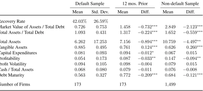
Table I presents these descriptive statistics. Using bothMarket Value of Assets / Total
Debt and Total Assets / Total Debt, defaulting firms are closer to insolvency compared
either to themselves 12 months prior to default or to the set of non-defaulting firms. Over
the 12 months leading up to default,Market Value of Assets / Total Debtfalls roughly three
times as muchTotal Assets / Total Debt, 73.2% versus 22.4%. TheMarket Value of Assets /
Total Debtratio of defaulting firms of 72.6% implies that roughly 30% of bondholder value
has been eroded by the firm remaining in business. This measure is broadly consistent with
Davydenko (2012) who finds that approximately 1/3of bondholder value is depleted by
shareholders prior to default and hints at a strategic motive behind default timing. Over this
period leading up to default, assets fall and firms write-down, or begin selling off, intangible
assets. Moreover, defaulting firms display cut backs in capital expenditures by 1.2% of firm
assets and 3.3% lower profitability. Interestingly, firms do not deplete their cash reserves in
the 12 months leading up to default. They do, however, display a shift away from long-term
liabilities and toward short term liabilities as debt maturity falls 20.9%. Compared to the
sample of non-defaulting firms, defaulting firms are smaller, less profitable, and have more
tangible assets. There is no statistically significant difference in the cash on hand between
defaulting firms and their non-defaulting counterpart.
1.3 Methodology
This section outlines the model and underlying assumptions used to estimate my main
results. I begin with an overview of a simple static model. Then, I build on that intuition
to develop a general dynamic model, which nests the model of Davydenko et al. (2012).
Next, I describe the estimation procedure to recover the parameters of interest. Finally, I
provide details on the empirical proxies that I use for the non-free parameters in the model.
1.3.1 Static Model
To develop intuition for my model, consider a simple one-period model of a firm’s
market value of assets just prior to default. In this case,
where M is the market value of the firm, V is the value of the firm’s assets, L is the
recovery value of the firm (ex-post), and q is the risk-neutral default probability. Simply
put, the market value of the firm is a convex combination of the continuation value of the
firm and the recovery value of the firm given default. This approach can be viewed as an
event study where the empiricist observes the market value of the firm just prior to default
and the market value of the firm just after default (the recovery value of the firm).
Thus for a given firm just prior to default, the market value of the firm’s assets,M, is
observed. Moreover, the ex-post recovery value of the firm,L, can be observed. Given an
estimate of the default probability of the firm,q, the continuation value of the firm,V, can
be calculated. Additionally, the cost of default is given byc=V −L.
As in Davydenko et al. (2012), identification in this model hinges on the assumption that
information about the firm’s fundamentals is incomplete, such that investors cannot know
with certainty that a firm will default in the next instant. In this setting as default occurs,
investors incorporate this information into prices and prices converge to their postdefault
recovery values. This identifying assumption is consistent with the large abnormal returns
observed empirically in papers such as Altman (1969); Clark and Weinstein (1983); and
Lang and Stulz (1992) who document shareholder losses of 20-30% following a firm’s
bankruptcy. In this imperfect information environment, Duffie and Lando (2001); Giesecke
(2006); and Jarrow and Protter (2004) show that a firm’s assets can be priced as though
default were a random event with a hazard rate that is a function of the firm’s economic
conditions. We review these dynamic pricing equations in the following subsection.
1.3.2 General Model
Consider the continuation value of a firm’s assets, Vt, which evolves following a
geo-metric Brownian motion,
where both the drift term and the volatility term can be time-varying. Moreover, let default
follow a heterogenous Poisson process with conditional risk-neutral intensity,λt.
Assum-ing that the recovery value of the firm, Lt, is a fraction of its continuation value, such
that
Lt= (1−αt)Vt,
the value of assets at time t∗ ≥ τ, where τ is the instant of default occurring prior to maturity, is given by:
Lt∗ = (1−ατ)VτEτ[e
Rt∗ τ rsds].
Denote T as the maturity date of the firm and f(τ) = λτ(Vτ)e−λτ as the instantaneous
hazard at timeτ. Under the risk-neutral measure,Q, the market value of the firm,Mt, for
t≤T can be written as follows
Mt=Et[e−
RT t rsds(V
T1{τ≥T} +
Z T
t
(1−ατ)VτEτ[e
RT
τ rsds]f(τ)dτ)]
=Et[e−
RT t rsds(V
TET[1{τ≥T}] +
Z T
t
(1−ατ)VτEτ[e
RT
τ rsds]f(τ)dτ)]
=Et[e−
RT t rsds(V
Te−
RT
t λs(Vs)ds +
Z T
t
(1−ατ)VτEτ[e
RT
τ rsds]f(τ)dτ)]
=Et[e−
RT
t rs+λs(Vs)dsV
T +e−
RT t rsds
Z T
t
(1−ατ)VτEτ[e
RT
τ rsds]f(τ)dτ]
=Et[e−
RT
t rs+λs(Vs)dsV
T +
Z T
t
e−RtTrsds(1−α
τ)VτEτ[e
RT
τ rsds]f(τ)dτ]
=Et[e−
RT
t rs+λs(Vs)dsV
T +
Z T
t
e−Rtτrsds(1−α
τ)Vτf(τ)dτ]
=Et[e−
RT
t rs+λs(Vs)dsV
T +
Z T
t
e−Rtτrsds(1−α
τ)Vτλτ(Vτ)e−λτ(Vτ)dτ].
(1.2)
assets, Mt, is a combination of the discounted value of the terminal value of the firm’s
assets,VT, times the probability that the firm does not default and the discounted value of
the instantaneous liquidation value,(1−ατ)Vτ, times the probability that the firm defaults
in the next instant.
In order to investigate cyclicality in the probability of default and default costs, I
con-sider ak×1vector of factors,xt, which govern the macroeconomy. These factors evolve according to a general transition equation
dx(t) =κ(µ−x(t))dt+ ΣdW(t). (1.3)
These factors feed into both the default hazard and the recovery value of the firm.
Specifi-cally, I make the following assumptions:
• The default hazard under the real probability measure is:
λP
t =e
−β0−β1logVtB−β2xt. (1.4)
Under this specification, the default hazard is a function of both some factors
(possi-bly latent risk factors) and observed firm characteristics. The default hazard
specifi-cation extends the default hazard model used in Davydenko et al. (2012) to include
a set of common economy-wide factors which impact the probability of a firm
de-faulting. Davydenko et al. (2012) use a firm’s economic solvency as a sufficient
statistic for default arguing that their assumption is common in structural models of
credit risk, such as Black and Cox (1976) and Merton (1974). Additionally, they
argue that firm solvency is a primary input in measures of default used by academics
and practitioners5, such as distance-to-default and Expected Default Frequency by
Moody’s/KMV, and is a strong predictor of firm default as shown empirically in
Davydenko (2012).
• The recovery value of the firm is a function of the underlying interest rate process:
αt=φ1+φ2xt. (1.5)
I make two additional assumptions for simplicity. However in Section 1.5, I confirm
that my results are not driven by either a constant default risk premium, ξ, or constant
volatility,σ.
• The intensity of the Poisson arrival process under the risk neutral measure is:
λQ
t =ξλPt (1.6)
• The value of the firm’s assets follows a geometric Brownian Motion with
time-varying drift under the risk neutral measure:
dVt=rtVtdt+σVtdWtQ (1.7)
The dynamic model I estimate is similar in spirit to the model proposed by Davydenko
et al. (2012) except that I relax several key assumptions that they make in order to test the
relationship between macroeconomic conditions and the joint determination of the
prob-ability of default and default costs. When firms face constant recovery rates and drift in
asset growth, Equation 2 further reduces to
Mt=Lt+ (Vt−Lt)EQt
VTe−r(t−t)
Vt
e−RtTλQudu
(1.8)
1.3.3 Factor Model
While my estimation allows for any of a broad class of general factors, I operationalize
the factors governing aggregate conditions using a standard two factor Gaussian model
given by:
r(t) =ϕ(t) +x(t) +y(t)
dx(t) =−ax(t)dt+σdW1(t)
dy(t) =−by(t)dt+ηdW2(t)
dW1(t)dW2(t) =ρ
This model is convenient for several reasons. First, it ties the underlying factor model to the
time-varying drift. Second, the factors can be estimated outside the model using the term
structure of US interest rates thus avoiding the additional computational burden of using a
Kalman filter within my estimation procedure.
Moreover, prior literature has emphasized the link between the term structure and the
macroeconomy. For example, Ang et al. (2006); Estrella and Mishkin (1998); and
Har-vey (1988) provide evidence that term structure factors predict future economic activity
(output). Similarly, Mishkin (1991) and Stock and Watson (2005) link information
em-bedded in the term structure to future inflation. Diebold et al. (2006) document that the
term structure effects future macro variables. Finally, Bekaert et al. (2010) ties the
infor-mational content of the yield curve to inflation targeting and monetary policy within a New
Keynesian framework.
These factors also carry important information regarding the liquidity preferences of
in-vestors. In theoretical work by Chen et al. (2013), bondholder liquidity demands drive
man-agers to delay bankruptcy despite the erosion of bondholder value during insolvency. Both
theoretical (for example, Brunnermeier and Pedersen (2009) and Chordia et al. (2001))
Longstaff (2004)) literature confirm the relationship between the term structure and bond
market liquidity. Specifically as investors demand more liquid, shorter-maturity bonds the
slope of the term structure increases.
1.3.4 Estimation
The estimation procedure follows Davydenko et al. (2012). Specifically, I employ an
expectation-minimization (E/M) algorithm to recover estimates for the parameters of
inter-est. The algorithm is as follows:
1. SetVt(1) =Mt.
2. Estimate hazard model given in Equation 4 usingVt(1).
3. Simulate new values of Vτ(2) for firm-months that correspond to default and use to
calculateα(2) = 1−L
τ/V
(2)
τ .
4. Estimate theφparameters by regressingα(2) onx
tandytand simulateV
(2)
t .
5. Iterate until parameters andVτ converge.
Since the expectations given in Equation 2 have no analytical solution, I numerically
solve for these expectations by simulating the path of the firm’s asset value over 10,000
draws.
1.3.5 Model Inputs
I compute the other variables that serve as model inputs as follows. Prior to default,
the market value of the firm, Mt, is estimated as the total value of all bonds, bank debt,
and common and preferred equity, as described in Section 2. The unit of observation is
firm-month due to data limitations. The value of the firm at default, Mτ, is approximated
by its value at the end of the last calendar month prior to default. Similarly, the recovery
value of the firm,Lτ, is observed at the end of the calendar month of default. To separate
subtract the market return from the defaulted firms return and adjust the recovery value of
assets accordingly.
The volatility of assets, σ, is the standard deviation of monthly asset returns for the
median firm in the industry, as follows. First, I estimate the standard deviation of each
firms monthly returns, as in Choi and Richardson (2009), excluding postdefault months
and firms with fewer than ten consecutive monthly firm value observations. Second, we
find the median asset volatility for the Fama French 17 Industry Classification. The use
of industry, rather than firm-specific, volatility estimates increases the number of usable
observations and reduces noise. Moreover, because the median firm in the industry is
typically not distressed, its firm and asset values are very close. Therefore, asset volatility
can be estimated as the volatility of the firm, which is much easier to measure, as it does
not have to be adjusted for unobserved expected default costs.
Debt maturity, T − t, is the weighted average of maturities of all debt instruments, assuming that all bank debt has a maturity of one year. The face value of debt, B, is the
total debt outstanding at the end of the previous fiscal quarter, as reported in CompuStat.
The factors underlying the risk-free rate rt are extracted from a two-factor Gaussian
term-structure model using the US Treasury yield curve and the no-arbitrage conditions.
1.4 Results
This section begins with some full sample tests in order to motivate the analysis and
highlight some of the identification problems that I face. These simple tests have the
ad-vantage of utilizing a broader sample of defaults for which market prices of bonds are not
available. After these tests, I present my main results.
1.4.1 Full Sample Tests
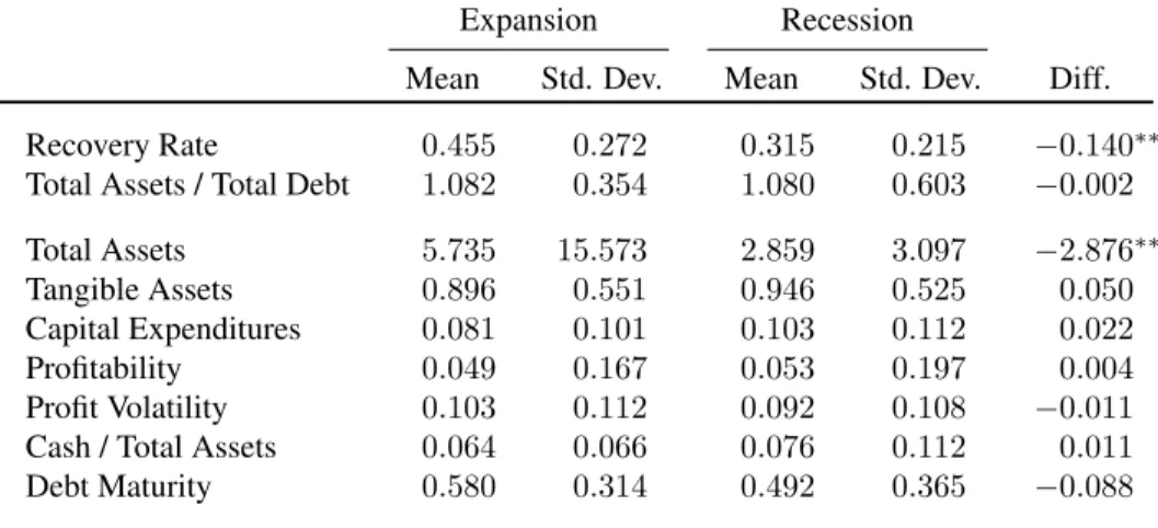
Table II presents the differences in defaulting firms across the business cycle as defined
by NBER recession dates. Two primary differences between these two sets of defaulting
the characteristics of defaulting firms being quite similar. While firms defaulting in
reces-sions are smaller than those firms defaulting during expanreces-sions, both sets of firms have
similar profitability, levels of tangible assets and profit volatility. This finding is consistent
with the notion that recovery rates vary through time rather than differences in the quality
of the firms defaulting in both states driving differences in sample composition between
the two groups of defaulting firms. Second, bankruptcies occur more frequently during
downturns despite the bankruptcy trigger being the same across the business cycle.
Simi-larly, cash on hand, a simple proxy for liquidity, does not differ significantly across the two
samples.
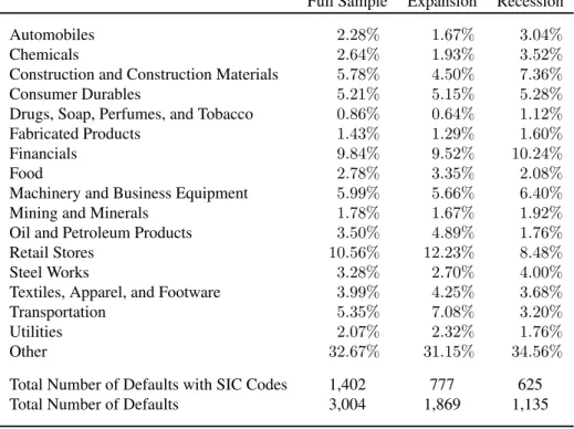
An alternative measure to assess the similarity of firms defaulting in good versus bad
economic states is to look at the industry composition of defaulting firms across the
busi-ness cycle. Panel A of Table III shows the percentage of defaulting firms by the 17 Fama
and French industries for the full sample of defaults and during both expansions and
reces-sions. On the whole, industry composition of defaulting firms is similar across the business
cycle providing further evidence that sample composition between the two groups of
de-faulting firms, firms dede-faulting in recessions and firms dede-faulting in expansions, is unlikely
the primary culprit in aggregate differences in recovery rates across the business cycle.
Insomuch as firms within a given industry are of a similar quality, differences in
aver-age recovery rates within an industry across different economic states are informative about
time-variation in recovery rates. While firm may differ in quality within an industry, asset
composition and exposure of those assets to aggregate productivity shocks are likely to be
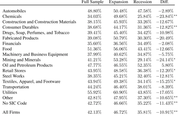
similar within industry. Panel B of Table III presents the differences in average recovery
rate within industry classification across the business cycle. Unlike in the industry
compo-sition of defaulting firms, recovery rates are consistently lower during economic downturns
within industry classification. For all firms within this broader sample of defaults,
differences in recovery rate range from a high of 24.14% lower recovery rates during
reces-sions in Mining and Minerals to a low of 10.65% lower recovery rates during recesreces-sions in
firms classified as Other Industries. The one industry in which recovery rates are not lower
during economic downturns is Oil and Petroleum Products; however, this difference is not
significantly different from zero.
I next turn to a multivariate analysis of recovery rates and default probabilities in
or-der to better control for differences in firm characteristics and sample composition through
time. For this analysis, I incorporate a continuous measure of the business cycle by
focus-ing on theLevelandSlopefactors of the term structure of interest rates rather than the
bi-nary NBER recession indicator. These continuous variables help me identify the transition
between recessions and expansions and provide a concise model for aggregate economic
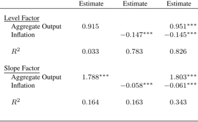
conditions in my main empirical analysis. Table IV presents parameter estimates from
re-gressions of these two factors on aggregate output and inflation. In the specifications using
both aggregate output and inflation, both theLevelandSlopefactor are positively related
to output and negatively related to inflation. Moreover, these two macroeconomic variables
do a relatively good job in explaining the variation in the two term structure factors. These
two macroeconomic variables explain 82.6% of the variation in theLevelfactor and 34.3%
of the variation in theSlopefactor. All told, macroeconomic conditions are highly related
to the continuous proxies I utilize in my analysis consistent with the more rigorous
empir-ical evidence of Ang et al. (2006); Estrella and Mishkin (1998); Harvey (1988); Mishkin
(1991); Stock and Watson (2005); and others.
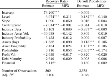
Table V presents the estimates from the regression of recovery rates on macroeconomic
conditions and a variety of controls. Consistent with time-varying recovery rates where
recovery rates fall during economic downturns,Levelis negatively and statistically
signif-icantly related to recovery rates. A one standard deviation increase in level is associated
aggregate and industry-levels of distress, Credit Spreadand Industry Profitability
respec-tively. These controls help to rule out an asset fire sale story to cyclicality in recovery rates
at either an aggregate-level, as in Altman et al. (2005), or at the industry-level, as in Shleifer
and Vishny (1992). Furthermore, firm characteristics meant to proxy for the quality of a
firm are not significantly related to recovery rates. This finding provides evidence against
sample composition being a primary driver in observed cyclicality in recovery rates.
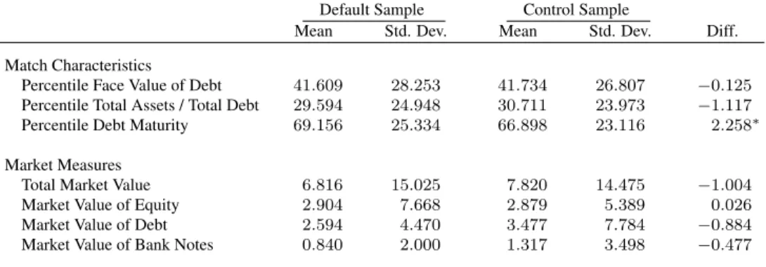
In order to examine the relationship between the business cycle and default
probabili-ties, it is important to examine only a set of firms likely to default in order to better isolate
the marginal impact of the variables of interest on default. To this end, I match the set
of defaulting firms to a control set of three non-defaulting firms per defaulting firm. The
match is made 12 months prior to default by minimizing the sum of the squared differences
in percentile face value of debt, percentileTotal Assets / Total Debt, and percentile debt
ma-turity. Non-defaulting firms are also required to be in the same industry as the defaulting
firm. Table VI presents the match quality between the defaulting and non-defaulting firms.
Along the dimensions of the match, defaulting and non-defaulting firms are quite similar
with the only statistically significant difference between the two groups being along the
dimension of debt maturity. In this case, non-defaulting firms have a shorter maturity of
debt, and thus as evidenced in Table I, be more likely, if anything, to default. Turning to
the capital structure of the defaulting firms versus that of the non-defaulting control group,
both groups exhibit a similar market value of assets and distribution of those assets between
equity, bonds, and bank notes.
While these simple tests provide preliminary evidence of the relationship between
macroeconomic conditions and recovery rates, it is important to note several shortcomings
of this approach. First, these straightforward tests use ex-post recovery data that combines
and the default decision is jointly determined. To this end, I follow the approach of
Davy-denko et al. (2012) in the next set of results. This methodology avoids these problems by
backing out the cost of default after observing the market value fo the firm just before and
just after bankruptcy is declared. Thus, the expectation of the recovery rate at the time of
default is recovered in this event study-like approach.
1.4.2 Estimates from Full Model
I now present the estimates from the full model detailed in Section 3.2. This analysis
overcomes many of the shortcomings of the prior analyses in order to better identify the
effects of macroeconomic conditions on both default probabilities and default costs. As
with the estimation framework of Davydenko et al. (2012), this methodology addresses the
joint estimation problem and recovers ex-ante estimates of default costs, which represent
the costs of financial distress rather than economic distress. Additionally, this estimation
procedure relaxes several key assumptions made in the Davydenko et al. (2012) case. First,
firm assets grow at a stochastic rate. Second, a firm’s default probability is a function of
its solvency as well as aggregate conditions. Third, a firm’s default costs are allowed to be
time varying within the estimation.
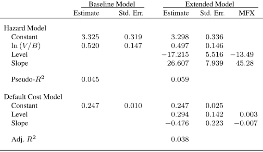
Estimates of both the baseline (Davydenko et al. (2012)) model and the extended model
are provided in Table VII. I begin with a discussion of the hazard model estimates, which
map firm solvency and macroeconomic conditions into the probability of a firm’s default.
Both proxies for macroeconomic conditions,LevelandSlope, are statistically significantly
related to the probability of default. A one standard deviation in the level of interest rates
is associated with firms liquidating 13 months earlier than in the case whereLevelis at the
mean. The slope of interest rates has an opposite effect on the survival probability of a firm.
A one standard deviation in theSlopeis associated with a delay of 45 months in the firm’s
default decision relative to the case where the slope of interest rates is at the mean. This
despite the destruction of bondholder value during insolvency, to the uncertainty regarding
the timing of cashflows from recovery due to asset lockup during bankruptcy proceedings.
When liquidity demands rise, investors buy more liquid, shorter-maturity bonds tilting the
slope of the yield curve up. Managers of insolvent firms postpone default relative to periods
in which the yield curve is flatter in order to provide liquidity to bondholders.
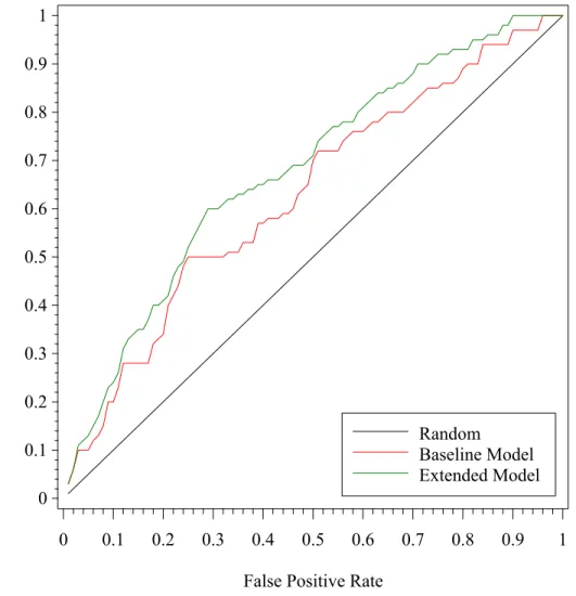
Figure I provides information on the fit of the hazard model augmented to control for
macroeconomic conditions. This figure plots the receiver operating characteristic (ROC)
curve to quantify the improvement in this model versus the baseline case where firm
sol-vency, as measured by the natural logarithm of firm value to the face value of debt, is a
sufficient statistic for characterizing the probability of a firm’s survival. This figure plots
the proportion of true positives classified correctly as such for a given threshold of false
pos-itives and aids in assessing model fit. For example allowing for 35 percent false pospos-itives,
the extended model that incorporates macroeconomic factors in addition to firm solvency
classifies 63 percent of the true positives correctly relative to 51 percent classified correctly
in the baseline model that uses firm solvency as a sufficient statistic to predict firm default.
Moreover, a statistically test of the area under the curve (AUC) for the two models rejects
the null of equal coverage at the 10 percent level. Taken together, the incremental effect of
including macroeconomic factors in the hazard model is statistically and economically
sig-nificant highlighting the importance of including factors related to aggregate bond market
liquidity in addition to firm characteristics when predicting firm default.
Now I turn to a discussion of the estimates of recovery rates as a function of
macroe-conomic conditions in the full model. Again, both proxies for macroemacroe-conomic conditions
are statistically significantly related to default costs. A one standard deviation inLevelis
associated with a 0.3% increase in the cost of default (decrease in recovery rate).
Con-versely, a one standard deviation increase in Slope is associated with a 0.7% decrease in
and a recession looms, cost of default rises asLevelfalls andSlopedecreases. Then as the
economy begins to recover and the term structure becomes upward sloped, cost of default
falls. This evidence is broadly consistent with the aggregate trends which motivate the
theoretical work by Chen (2010). Moreover insomuch as the quality of defaulting firms is
similar across the business cycle, as argued in Section 1.4.1, these results provide evidence
of time-variation in the cost of default. However, the magnitudes of these macroeconomic
effects are much smaller than the trends apparent from aggregate data, hinting that the
qual-ity of assets of defaulting firms may still play a role. Additionally, these tests provide little
evidence as to the drivers of this time-variation in recovery. For example, aggregate
dis-tress or industry-specific disdis-tress that is tied to macroeconomic conditions may lead to asset
fires sales as in Altman et al. (2005) or Pulvino (1998), and the full model estimates are
simply picking up these effects. In the next section, we explore a battery of additional tests
designed to rule out these and other potential alternative explanations for these findings.
Among other tests, we better control for the quality of defaulting firms as well as provide
evidence that distress in non-defaulting firms/asset fire sales are not the primary drivers of
these results.
1.5 Additional Tests
In this section, I address the robustness of my findings to several potential concerns.
First, I consider sequential estimates which allow controls for additional aggregate and
firm-specific controls. Next, I consider the case in which the jump intensity of default
arrival varies through time and the case in which firm asset volatility is time varying. Then,
I consider the relationship between aggregate and industry-level distress and the default
probability. I conclude this section by examining the effects of time-varying recovery rates
on the timing of a firm’s default and examining the bond pricing implications of
1.5.1 Sequential Estimates
Unfortunately, the inclusion of additional variables in my estimation requires
specify-ing a law of motion for each variable so that investors can form expectations of the future
values of these variables. Instead of harnessing my estimation procedure with this
addi-tional complexity, I address the problem of omitted variables that are correlated with my
proxies for macroeconomic conditions by performing a sequential estimation procedure.
Specifically in this subsection, I follow the approach of Davydenko et al. (2012) and
esti-mate a nested case of the full model in which assets grow at a constant rate, firm solvency
is a sufficient statistic for estimating default probabilities, and firms face constant default
costs. This model is the baseline model presented in Table VII. I then examine the
rela-tionship between these first-stage estimates and the battery of macroeconomic variables,
firm-characteristics, and aggregate and industry-level controls used in Tables V. While this
approach faces a number of unrealistic assumptions, estimates from these results are
con-sistent with the results from the full sample of defaults. Moreover, these results address
the use of ex-post recovery rate data and the joint determination of the default decision and
recovery rates.
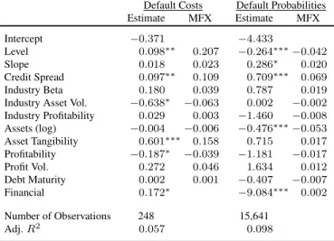
Table VIII presents the analogue of Table V within the Davydenko et al. (2012)
esti-mation framework. In this table, the dependent variable are firm-level estimates ofDefault
Costs= (1−Recovery Rate) recovered from the estimation procedure described in Section 3.2. Similar to the OLS results presented in Table V,Level is positively (negatively) and
statistically significantly related to default costs (recovery rates). After controlling for the
expectation of default costs rather than the ex-post realization of financial distress costs and
the joint estimation problem, the impact of macroeconomic conditions on default costs is
roughly a third lower with a one standard deviation increase inLevel corresponding to a
one third of default costs estimated in the OLS case are attributable to the costs of
eco-nomic, rather than financial, distress. As before, aggregate distress, as measured byCredit
Spread, is positively and statistically significantly related to default costs. However, these
estimates are roughly two-thirds smaller than in the OLS case. Again, this finding is
con-sistent with a large portion of OLS estimates of default costs (recovery rates) attributable
to economic versus financial distress costs. Within this estimation framework, several
vari-ables proxying for asset quality are statistically significantly related to default costs. Firms
with more profitable assets face lower expected default costs with a one standard
devia-tion increase in profitability being associated with an almost 4% decrease in default costs.
Firms with higher industry-level asset volatility interestingly exhibit lower default costs as
well. A one standard deviation increase in asset volatility is associated with a roughly 6%
decrease in default costs. Finally, firms with higher asset tangibility face higher expected
default costs. A one standard deviation increase in asset tangibility is associated with a
roughly 16% increase in default costs.
1.5.2 Time-varying Jump Intensity
One potential concern of my estimates is that the inclusion of macroeconomic
condi-tions in the hazard model simply captures variation through time in the mapping of the
Poisson arrival process for firm default between the real probability (P) measure and the
risk neutral (Q) measure. To address this concern, I allow the jump intensity measure
presented in Equation 5 to vary through time. Thus,
λQ
t =ξtλPt.
In order to identifyξt, I estimate the Volatility Risk Premium for each month in the spirit
of Bollerslev et al. (2009) and Drechsler and Yaron (2011). Specifically,ξtis equal to the
ratio of the model-free expected volatility as measured by the VIX index and the realized
then rescale this measure to ensure that the jump intensity is greater than one in all months.
This proxy provides a time-varying measure of jump intensity that may helps alleviate
concerns that significant loadings on macroeconomic conditions in the hazard model for
firm default, β2 and β3, are simply picking up variation in jump intensity through time.
Results from this specification are presented in the second set of results in Table IX. The
estimates of cyclicality in default probabilities and recovery rates are quantitatively similar
to the main results presented in Section 5.3.
1.5.3 Time-varying Volatility
A rich literature has developed regarding time-variation in firm volatility, for example
Engle (1982); Bollerslev (1986); Bakshi et al. (1997); Chernov and Ghysels (2000) and
cites therein. Systematic measurement error in firm volatility may distort estimates of the
probability of default and the costs of default. For example, volatility may be systematically
high during economic downturns as in Nelson (1991). As the economy recovers, firm
volatility may drift downward to an expected long-term mean. Thus in the estimation,
firm volatility is overstated leading to estimates of firm default probabilities that are biased
upward and correlated with recessionary conditions. Similarly, estimates of firm default
costs are biased downward and correlated with recessionary conditions.
To account for this time-variation in firm asset volatility, I allow the value of the firm’s
assets to follow the geometric Brownian motion under the risk neutral measure below:
dVt=rtVtdt+σtVtdWtQ
σt= (1−α)¯σ+ασt−1
This concise representation of time-varying firm volatility follows the spirit of the GARCH
literature of Engle (1982) and Bollerslev (1986), while minimizing the number of extra
pa-rameters to be included in the model. Specifically, I estimate a centered 24-month standard
These industry estimates provide firm-levelαandσ¯. σtfor a given firm-month is calculated
as in the main results.
Specifying volatility in this manner allows firm volatility to return to the level of
long-run expected volatility for the industry to which the firm belongs despite temporary
move-ments away from this long-term mean of volatility and should reduce the potential for
volatility-related biases in the probability of default and default cost estimates. Results for
this time-varying volatility specifications are presented in the third set of estimates in Table
IX and are quantitatively similar to the main results.
1.5.4 Aggregate and Industry-level Distress
Similar to the above concerns, time variation in the level of aggregate distress as in
Altman et al. (2005) or in the level of industry distress as in Shleifer and Vishny (1992)
that is correlated with macroeconomic conditions may distort estimates of the cyclicality
of default probabilities and default costs. To address this concern, I control for this distress
within the estimation by augmenting the default cost specification to include the aggregate
or industry-level default probability as a proxy for the level of distress. Specifically, a firm’s
recovery rate is
αt=φ1+φ2xt+φ3yt+φ4λ−i,t,
where
λ−i,t =
1
n X
j∈−i
λj,t =
1
n X
j∈−i
e−β0−β1log
Vj,t
Bj −β2xt−β3yt.
This sum is taken over all firms in the sample excluding firm i to proxy for aggregate
distress or over all firms in the same industry as firmiexcluding firmito proxy for
industry-level distress. The primary advantage of this proxy for distress is that it is internal to the
Table IX presents the results from this estimation. Again, parameter estimates are
sim-ilar to those obtained from the estimation, which does not explicitly control for distress at
the aggregate or industry-level. This evidence is broadly consistent with time-variation in
a given firm’s recovery rate that is related to macroeconomic conditions rather than asset
liquidity or fire sales.
1.6 Conclusion
My study attempts to provide an answer to the following question: do default costs
vary across the business cycle or are aggregate measures of default costs simply picking
up differences in asset quality (sample composition)? While this time variation is apparent
in simple multivariate regressions of firm default and recovery rates on macroeconomic
conditions and a battery of industry and firm-specific characteristics, it is important to strip
out the cost of economic distress by focusing on investor’s expectations of recovery rates
rather than ex-post measures of recovery. Additionally, the default decision and recovery
rates are jointly determined, which may induce bias in parameter estimates from simple
regressions. By exploiting changes in the market value of a firm’s assets around default
events, I estimate the role of business cycle conditions on the joint determination of ex-ante
default costs and the default probability of the firm.
I find evidence that is consistent with time-variation in default costs within a given firm.
Specifically, a one standard deviation increase in the level of interest rates is associated with
a 0.3% increase in the cost of default (decrease in recovery rate) and with firms liquidated
13 months earlier than the case of no change in interest rates. Moreover, a one standard
deviation increase in the slope of interest rates is associated with a 0.7% decrease in the
cost of default (increase in recovery rate) and with firms delaying the default decision 45
months than in the case of no change in interest rates.
These findings are broadly consistent with firms facing time-varying recovery rates
effect where firms with low quality assets face financial distress costs during economic
downturns. However, the economic effects are relatively small compared to the economic
effects of the delay in bankruptcy when facing poor macroeconomic conditions. This
strate-gic bankruptcy story is consistent with the theoretical model of Chen et al. (2013) in which
bondholder liquidity demands incentivize the firm to remain an ongoing concern.
Specifi-cally as investors demand more liquid, shorter-maturity bonds the slope of the term
struc-ture increases and firms delay bankruptcy in order to provide bondholders liquidity.
Moreover, my findings are robust to a variety of additional tests. First, I consider
se-quential estimates which allow controls for additional aggregate and firm-specific controls.
Next, I consider the case in which the jump intensity of default arrival varies through time
and the case in which firm asset volatility is time varying. Then, I consider the relationship
between aggregate and industry-level distress and the default probability.
Future research should explore the pricing implications of these micro-level findings.
Spreads from corporate structural models incorporating both time-variation in recovery
rates and in default probabilities can be compared to spreads observed in the data. One
natural extension of this work is to incorporate the estimates of the time-variation in distress
risk to further explore the panel of bond returns in the context of a constant credit cost
component, a time-varying credit cost component, and firm-specific COAS.
Similarly, additional research should explore the relationship between the components
of distress risk I explore, probability of default and default costs, as they relate to equity
returns. While a host of papers explore the pricing of distress risk in equities (Kapadia
(2011); Ogneva et al. (2014); among others), some puzzling findings still remain, which
the decomposition of time-varying distress risk into time-variation in the probability of
Figure 1.1: Receiver Operating Characteristic Curve
This figure plots the receiver operating characteristic curve for the hazard model estimated in Table VII. For a given threshold of false positives, the percentage of true positives identified by the fitted model is plotted. The baseline model, in which firm solvency is a sufficient statistic for default, is plotted in red. The extended model, in which firm solvency is augmented with macroeconomic factors, is plotted in green.
T
ru
e
P
o
s
it
iv
e
R
a
te
0 0.1 0.2 0.3 0.4 0.5 0.6 0.7 0.8 0.9 1
False Positive Rate
0 0.1 0.2 0.3 0.4 0.5 0.6 0.7 0.8 0.9 1
Table 1.1: Summary Statistics
This tables presents summary statistics for the sample of defaulting firms in the month of default, the sample of defaulting firms twelve months prior to default, and the sample of non-defaulting firms. For the sample of non-defaulting firms, I present the cross-sectional mean of the time-series median of the firm characteristic. Recovery Rate is the equally-weighted average price relative to par for defaulting issues 30 days after default.Market Value of Assets / Total Debtis the ratio of the market value of firm assets to total face value of debt (LTQ).Total Assets / Total Debtis the ratio of the total book value of assets (ATQ) to total face value of debt. Total Assetsis the total book value of assets in billions of dollars.Tangible Assetsis the the ratio of plants, property, and equipment (PPEGTQ) to total book value of assets. Capital Expenditures is total of the previous 4 quarters of capital expenditures6scaled by total assets. Profitabilityis the sum of the previous 4 quarters of operating income before depreciation (OIBDPQ) divided by the sum of the previous 4 quarters of net sales (SALEQ).Profit Volatility is the 5-year centered standard deviation ofProfitability. Cash / Total Assetsis the ratio of cash and short-term investments (CHEQ) to total assets. Debt Maturityis the ratio of long-term liabilities (LLTQ) to total liabilities (LTQ). For the test of the difference in means, ∗, ∗∗,and∗∗∗denote significance at the 10 percent, 5 percent and 1 percent levels, respectively.
Default Sample 12 mos. Prior Non-default Sample
Mean Std. Dev. Mean Diff. Mean Diff.
Recovery Rate 42.03% 26.59%
Market Value of Assets / Total Debt 0.726 0.753 1.458 −0.732∗∗∗ 2.849 −2.123∗∗∗
Total Assets / Total Debt 1.093 0.431 1.317 −0.224∗∗∗ 1.652 −0.559∗∗∗
Total Assets 6.262 17.253 7.156 −0.894∗∗∗ 10.759 −4.497∗∗
Tangible Assets 0.885 0.495 0.761 0.124∗∗∗ 0.626 0.260∗∗∗
Capital Expenditures 0.081 0.093 0.094 −0.012∗ 0.067 0.015
Profitability 0.054 0.173 0.087 −0.033∗∗ 0.147 −0.094∗∗
Profit Volatility 0.094 0.105 0.098 −0.004 0.079 0.015
Cash / Total Assets 0.068 0.080 0.079 −0.011 0.076 −0.008
Debt Maturity 0.563 0.327 0.772 −0.209∗∗∗ 0.684 −0.121∗∗∗
Table 1.2: Differences in Defaulting Firms Across the Business Cycle
This tables presents differences in the characteristics of defaulting firms conditional on whether default occurs during an NBER recession. Recovery Rateis the equally-weighted average price relative to par for defaulting issues 30 days after default. Market Value of Assets / Total Debt is the ratio of the market value of firm assets to total face value of debt (LTQ).Total Assets / Total Debt is the ratio of the total book value of assets (ATQ) to total face value of debt. Total Assets
is the total book value of assets in billions of dollars. Tangible Assets is the the ratio of plants, property, and equipment (PPEGTQ) to total book value of assets. Capital Expendituresis total of the previous 4 quarters of capital expenditures7scaled by total assets.Profitabilityis the sum of the previous 4 quarters of operating income before depreciation (OIBDPQ) divided by the sum of the previous 4 quarters of net sales (SALEQ).Profit Volatilityis the 5-year centered standard deviation ofProfitability. Cash / Total Assetsis the ratio of cash and short-term investments (CHEQ) to total assets. Debt Maturityis the ratio of long-term liabilities (LLTQ) to total liabilities (LTQ). For the test of the difference in means,∗, ∗∗,and∗∗∗denote significance at the 10 percent, 5 percent and 1 percent levels, respectively.
Expansion Recession
Mean Std. Dev. Mean Std. Dev. Diff.
Recovery Rate 0.455 0.272 0.315 0.215 −0.140∗∗
Total Assets / Total Debt 1.082 0.354 1.080 0.603 −0.002
Total Assets 5.735 15.573 2.859 3.097 −2.876∗∗
Tangible Assets 0.896 0.551 0.946 0.525 0.050
Capital Expenditures 0.081 0.101 0.103 0.112 0.022
Profitability 0.049 0.167 0.053 0.197 0.004
Profit Volatility 0.103 0.112 0.092 0.108 −0.011
Cash / Total Assets 0.064 0.066 0.076 0.112 0.011
Table 1.3: Default Statistics by Industry - Full DRD Sample
This tables presents default statistics by industry. Expansionary and recessionary periods are classi-fied using the NBER recession dates. Panel A provides the distribution of defaults across 17 Fama and French industries. Panel B presents the mean recovery rate by Fama and French 17 Industry Classification.Recovery Rateis the equally-weighted average price relative to par for defaulting is-sues 30 days after default. For the test of the difference in means between defaults occuring within recessionary periods versus those occuring during periods of expansion,∗, ∗∗,and∗∗∗denote sig-nificance at the 10 percent, 5 percent and 1 percent levels, respectively.
Panel A: Frequency of Defaults
Full Sample Expansion Recession
Automobiles 2.28% 1.67% 3.04%
Chemicals 2.64% 1.93% 3.52%
Construction and Construction Materials 5.78% 4.50% 7.36%
Consumer Durables 5.21% 5.15% 5.28%
Drugs, Soap, Perfumes, and Tobacco 0.86% 0.64% 1.12%
Fabricated Products 1.43% 1.29% 1.60%
Financials 9.84% 9.52% 10.24%
Food 2.78% 3.35% 2.08%
Machinery and Business Equipment 5.99% 5.66% 6.40%
Mining and Minerals 1.78% 1.67% 1.92%
Oil and Petroleum Products 3.50% 4.89% 1.76%
Retail Stores 10.56% 12.23% 8.48%
Steel Works 3.28% 2.70% 4.00%
Textiles, Apparel, and Footware 3.99% 4.25% 3.68%
Transportation 5.35% 7.08% 3.20%
Utilities 2.07% 2.32% 1.76%
Other 32.67% 31.15% 34.56%
Total Number of Defaults with SIC Codes 1,402 777 625
Table 1.3: Default Statistics by Industry - Full DRD Sample (cont.)
Panel B: Average Recovery Rate
Full Sample Expansion Recession Diff.
Automobiles 48.80% 50.48% 47.58% −2.89%
Chemicals 34.03% 49.68% 25.84% −23.84%∗∗
Construction and Construction Materials 38.15% 45.93% 33.26% −12.67%
Consumer Durables 38.68% 44.17% 31.36% −12.82%∗∗
Drugs, Soap, Perfumes, and Tobacco 39.41% 45.40% 34.42% −10.98%
Fabricated Products 39.08% 50.79% 30.30% −20.49%
Financials 35.60% 36.56% 34.49% −2.08%
Food 51.36% 56.06% 43.41% −12.66%
Machinery and Business Equipment 37.99% 40.62% 34.87% −5.75%
Mining and Minerals 41.21% 53.28% 29.14% −24.14%∗
Oil and Petroleum Products 47.77% 46.55% 52.35% 5.80%
Retail Stores 43.95% 48.58% 36.38% −12.20%∗
Steel Works 38.35% 45.21% 32.40% −12.81%
Textiles, Apparel, and Footware 43.94% 49.38% 34.14% −15.25%∗
Transportation 44.24% 46.40% 38.01% −8.39%
Utilities 55.92% 60.90% 43.85% −17.05%
Other 42.81% 47.95% 37.30% −10.65%∗∗∗
No SIC Code 42.72% 46.66% 35.22% −11.43%∗∗∗
Table 1.4: Term Structure and Output
This tables presents parameter estimates from the regression of theLevelandSlopefactor on Aggre-gate OutputandInflation. Levelis the first factor extracted from fitting a two-factor Gaussian term structure model to the US Treasury yield curve. Slope is the second factor extracted from fitting a two-factor Gaussian term structure model to the US Treasury yield curve. Aggregate Output is the natural logarithm of real GDP.Inflationis the year-over-year log change in CPI. Standard errors are robust to heteroskedasticity. ∗,∗∗and∗∗∗ denote significance at the 10 percent, 5 percent and 1 percent levels, respectively.
Estimate Estimate Estimate
Level Factor
Aggregate Output 0.915 0.951∗∗∗ Inflation −0.147∗∗∗ −0.145∗∗∗
R2 0.033 0.783 0.826
Slope Factor
Aggregate Output 1.788∗∗∗ 1.803∗∗∗ Inflation −0.058∗∗∗ −0.061∗∗∗
Table 1.5: Simple Regressions
The first two columns of this table present the parameter estimates from the regression of recovery rates on macroeconomic variables, industry characteristics and firm characteristics. The last two columns of this table present the parameter estimates from the logit regression modeling the prob-ability of default for defaulting firms and the matched sample of non-defaulting firms. Recovery Rateis the equally-weighted average price relative to par for defaulting issues 30 days after default.
Levelis the first factor extracted from fitting a two-factor Gaussian term structure model to the US Treasury yield curve. Slopeis the second factor extracted from fitting a two-factor Gaussian term structure model to the US Treasury yield curve. Other variables are defined in the text. Marginal effects are the change in the dependent variable for a one standard deviation change in the inde-pendent variable. Standard errors are robust to firm-level heteroskedasticity. ∗, ∗∗ and∗∗∗ denote significance at the 10 percent, 5 percent and 1 percent levels, respectively.
Recovery Rates Default Probabilities Estimate MFX Estimate MFX
Intercept 73.260∗∗∗ −0.609
Level −3.974∗∗∗−0.311 −0.182∗∗∗−0.140 Slope −1.090 −0.050 0.016 0.004 Credit Spread −7.014∗∗∗−0.301 −0.044 −0.010 Industry Beta 10.163 0.080 −0.837∗∗ −0.063 Industry Asset Vol. −39.938 −0.142 0.809 0.019 Industry Profitability −3.453 −0.012 0.009 −0.007 Assets (log) −1.558 −0.090 0.115∗∗∗ 0.105 Asset Tangibility 2.434 0.024 1.131∗∗∗ 0.105 Profitability 6.716 0.053 −2.405∗∗∗−0.174 Profit Vol. −2.639 −0.017 −0.820 −0.020 Debt Maturity −2.649 −0.029 0.008 −0.006 Financial −8.112∗ 0.130 0.002
Number of Observations 560 2,538