An Empirical Comparison of Meta-Modeling
Techniques for Robust Design Optimization
Sibghat Ullah
1, Hao Wang
1, Stefan Menzel
2, Bernhard Sendhoff
2, and Thomas B¨ack
11
Leiden Institute of Advanced Computer Science (LIACS), Leiden University, The Netherlands
Email:
{
s.ullah,h.wang,t.h.w.baeck
}
@liacs.leidenuniv.nl
2
Honda Research Institute Europe GmbH (HRI-EU), Offenbach/Main, Germany
Email:
{
stefan.menzel,bernhard.sendhoff
}
@honda-ri.de
Abstract—This research investigates the potential of using meta-modeling techniques in the context of robust optimization namely optimization under uncertainty/noise. A systematic em-pirical comparison is performed for evaluating and comparing different meta-modeling techniques for robust optimization. The experimental setup includes three noise levels, six meta-modeling algorithms, and six benchmark problems from the continuous optimization domain, each for three different dimensionalities. Two robustness definitions: robust regularization and robust composition, are used in the experiments. The meta-modeling techniques are evaluated and compared with respect to the model-ing accuracy and the optimal function values. The results clearly show that Kriging, Support Vector Machine and Polynomial regression perform excellently as they achieve high accuracy and the optimal point on the model landscape is close to the true optimum of test functions in most cases.
Keywords—meta-modeling, surrogate-assisted optimization, ro-bust optimization, quality engineering, machine learning
I. INTRODUCTION
U
ncertainty is an imperative motif in design optimization. The classical view on black-box optimization does not account for these uncertainties. It is important to state that throughout this paper uncertainty and noise refer to the same concept, (i.e., unexpected drifts in the optimization setup). These unexpected drifts can be found in the design and envi-ronmental parameters, e.g., temperature, stiffness, structural rigidity etc. as well as in the constraints and objectives. Accounting for these uncertainties leads to the concept of robust design optimization aka quality engineering [1]. Re-cently, many methodologies have been investigated for robust optimization. Most of these approaches for robust optimization focus on using direct search methods, in particular evolution strategies and surrogate-assisted (aka meta-model based) opti-mization. We believe that while the former has been discussed at length in the context of robust optimization [2]–[7], the latter still needs further consideration. In particular, the practical ar-eas of interest regarding the computational tractability, fidelity and flexibility of meta-model based optimization need to be investigated [8]–[10].Uncertainties and noise comprise one of the most chal-lenging areas in optimization literature. They are encoun-tered frequently in real-world optimization problems. These notions are significant in engineering optimization such as
automobile manufacturing, building construction and steel production due to the potentially serious impact in case of a failure. As such, achieving robustness in design optimization is important. Despite the significance, achieving robustness in design optimization is challenging. We believe this is due to the veracity of optimization landscapes, high dimensionality and the intrinsic complexity of product life cycle. On the other hand, computational statistics based supervised learning methods have been successfully employed in Artificial In-telligence applications in health-care, transportation, banking and finance, signal processing, multimedia and entertainment. As such, it is desirable to investigate the suitability of these methods to help designing robust systems.
For many reasons, incorporating robustness in design opti-mization is challenging. Firstly, uncertainty has many shapes and forms [7], [11]. The nature and structure of uncertainty is often unknown in advance. Secondly, uncertainty has many sources [7], [11] such as environmental and design parameters, objectives and constraints. Thus, accounting for all sources of uncertainty in an accurate fashion is often impossible. Thirdly, uncertainty modeling and representation is itself quite tedious and exhaustive. Finally, there is lack of cohesive literature to minimize the effects of all types of uncertainty and design a robust system. As such, it is desirable to obtain practically useful insights to be adopted by engineers to account for the unexpected changes during optimization.
mathematical programming techniques are discernible [11] as they are not naturally associated with simulation which forms an important part of the optimization pipeline in engineering [17]. Also, this family of techniques are hardly flexible and analytically tractable in most real-world design optimization tasks. The combination of the robust-counterpart approach with direct search methods is usually focusing on evolutionary algorithms only. As such, we believe there is a dire need for combining the robust-counterpart approach with intelligent, experience based optimization schemes such as meta-model based optimization which are easy to model, appraise and practice.
In this paper, we study sensitivity robustness [18], [19], i.e., robustness related to the sensitivity w.r.t. noise on the design parameters. We use six optimization problems. We then construe three levels of additive noise characterizing small, medium and big uncertainty during optimization. Furthermore, to incorporate robustness for the corresponding noisy func-tions, we choose two robust-counterpart approaches, namely the robust regularization based on the worst case scenario and the robust composition, i.e., robustness achieved through combining the expectation and dispersion of a noisy function. As a result, we have thirty-six noisy optimization cases due to three levels of noise and two robust-counterpart approaches. We study six meta-modeling techniques: Kriging, Support Vector Machines (SVM), Radial Basis Function Network (RBFN), Random Forest (RF), K Nearest Neighbors (KNN) and Elastic net with second order polynomial regression func-tion (ELN). We perform hyper-parameter optimizafunc-tion of the corresponding hyper-parameters for all meta-modeling algorithms, to obtain the best results for each scenario. Conclusively, we evaluate and compare these meta-modeling techniques on these test cases and discuss their generality, reliability, and computational tractability.
The rest of the paper is organized as follows. We present the idea of robustness in design optimization in section II. This includes robust counter-part approaches namely the robust regularization and robust composition discussed in section II-A and section II-B respectively. Section III provides a brief introduction to meta-modeling. In section IV, we present the experimental design for this work. This is followed by results in section V. Finally, we discuss the logical conclusion of the paper along-side the future research line in section VI.
II. ROBUSTNESS IN BLACK-BOX OPTIMIZATION
In this work, we consider real-valued black-box optimiza-tion problems f: S → R, with S ⊆ Rd, where the so-called feasible region S is specified by inequality constraints
gj(x) ≤ 0 (j ∈ {1, . . . , J}) and equality ones hk(x) = 0
(k ∈ {1, . . . , K}), x ∈ S. Without loss of generality, the
objective function f is subject to minimization. In most real-world design optimization tasks, the objective and constraint functions are non-linear.
One of the key problems in solving the optimization is to handle the uncertainty, since in practice, the evaluation of inputs can introduce noises and even the objective function
could be dynamic in time. As an example, environmental parameters such as pressure, humidity etc. vary unexpectedly at times. Likewise, design parameters can fluctuate because of floating point arithmetic, division by zero and quality compromises which are associated with high precision costs in manufacturing [11]. Furthermore, the systematic errors are unavoidable in the modeling of physical processes.
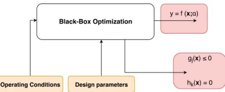
An example of an optimization problem with various sources of uncertainty is illustrated in figure 1. Uncertainties in parameters are related with sensitivity robustness [18], [19] whereas uncertainty in objectives and constraints is strongly linked with reliability [20], [21] and feasibility robustness [22]. Parameters in a design optimization problem can be classified into two types, namely design and environmental ones. Incorporating robustness in design optimization with respect to these parameters leads to the concept of sensitivity robustness. The effect of additive noise δx ∈ Rd in design parameters of an objective function is formulated in Eq. (1) wheref˜(x)is the noisy counter-part of an arbitrary objective functionf(x).
˜
f(x) =f(x+δx) (1)
Additionally, the operational or environmental conditions fluctuate or are known only to a certain extent. This means that our existing knowledge about the system is limited. In the classical optimization setting, environmental conditions are treated as constants. However, considering the different phases of the product life cycle that is hardly the case in a practical application. We thus extend the output dependency to the environmental variables setCwhereα∈ Crepresents an individual environmental variable. The effect of such additive noise δα ∈ R on the output of an objective function is represented in Eq. (2).
˜
f(x;α) =f(x;α+δα) (2)
In this work, we employ the robust counter-part approach [16] to achieve robustness. The idea behind the robust counter-part approach is to reformulate the optimization problem in a way so as to minimize the effect of parametric uncertainties
δxandδα in Eqs. (1) and (2). Hence, it is important to model
δx andδα to design a robust system. The robust counter-part approach also requires to reformulate the optimization goal, i.e., whether to optimize the expected or worst case behavior of the objective function. Further, the constraint functions are revised to design a robust counter-part which by definition includes the robustness w.r.t. parametric imprecision. Finally, the resulting robust counter-part is substituted in place of the original problem and solved using any optimization methodol-ogy of interest. We study two robust counter-part approaches, namely the robust regularization and robust composition.
A. Robust Regularization
Black-Box Optimization
Operating Conditions Design parameters
y = f (x;α)
gj(x) ≤ 0
hk(x) = 0
Fig. 1. An example of a constrained, single-objective design optimization problem with four common sources of uncertainty (i.e., design and environ-mental parameters in orange shade rectangles, objective and constraints in orchid shade rectangles).
counter-part approach first defines a neighbourhood N(x) of design x whose size is determined by the parameter
[13]. Then, an upper-bound of f(x)is defined by taking into account the worst value of design x including neighborhood
N(x). Finally, the optimization goal is characterized so as to minimize this upper bound. The minimum returned by using this strategy is called “least upper-bound”. Formally, the robust counter-partR(x)based on robust regularization is defined in Eq. (3).
R(x) = sup
ξ∈N(x)
f(ξ) (3)
The optimization goal then becomes to solve Eq. (3). This approach is called robust regularization because in Eq. (3) acts as a regularization parameter (i.e., defines the size of the neighbourhood).
B. Robust Composition
Robust regularization is a theoretically stable strategy to design systems with sensitivity robustness and has been dis-cussed in operations research [16]. Different from robust regularization, engineers can also optimize the expected output of a noisy function E[ ˜f(x)]while minimizing the dispersion
(V[ ˜f(x)])0.5simultaneously. We refer to it as robust
composi-tion similar to [8]. Robust composicomposi-tion requires the uncertainty
δx be specified in the form of a probability distribution. The expectation E[ ˜f(x)] and dispersion (i.e., standard deviation)
(V[ ˜f(x)])0.5of the noisy function are combined at each point x in S to produce a robust scalar output. The optimization goal thus becomes to find a point x∗ in S which minimizes this scalar. The robust counter-part with robust composition is defined in Eq. (4). In this paper, we assume δx ∼ N(0, σ2) whereσ2depends on the range of parameters and noise level.
minimize R(x) =E[ ˜f(x)] + q
V[ ˜f(x)]
˜
f(x) =f(x+δx) (4)
δx∼ N(0, σ2)
III. META-MODELING INOPTIMIZATION
The idea of using a simple empirical approximation to substitute a complex model was proposed as early as 1974
[24]. This line of research was particularly used in structural optimization [25]–[29] with the name of Response Surface Ap-proximation. The first attempt to classify such methodologies based on their accuracy in the context of structural engineering was made in 1993 [30]. On the other hand, the first significant attempt to replace a deterministic computer simulation with a meta-model was presented in [31]. Meta-modeling for robust design optimization has been investigated in [8], [9], [32]–[35]. For a detailed review of meta-modeling and its applications in structural engineering, the reader is directed to [8].
The idea behind meta-modeling is to build an empirical approximation model fˆ(x) of an objective function f(x). The approximation fˆ(x) then acts as the meta-model (aka surrogate-model) off(x). This abstraction is useful in a variety of situations. Firstly, it simplifies the task to a great extent in simulation based modeling and optimization. Secondly, it provides the engineer with an opportunity to evaluate f(x)
indirectly if the exact computation of f(x) is too costly or complex. Additionally, it provides the engineer with practically useful insights. Meta-modeling first evaluates f(x)at several points of interest(x1,x2, . . . ,xN), e.g., using Latin hyper-cube
sampling, Plackett-Burman [36], Box-Behnken [37] design etc., and generates the data set of input{x1,x2, . . . ,xN} and
output {f(x1), f(x2), . . . , f(xN)} pairs, i.e., sample points
and resulting function values. The data generated can then be used to build a nonlinear regression model for approximating the objective functionf(x). In principle, any regression based machine learning methodology (e.g., Kriging, neural networks, polynomials etc.) may be used. Since no regression model can perfectly approximate the original functionf(x)by means of a limited number of evaluations, the resulting meta-modelfˆ(x)
will be relatively inaccurate.
Although meta-modeling is relatively easy to use compared to classical optimization, it must be carefully designed. Firstly, selecting the set of points {x1,x2, . . . ,xN} to evaluate f(x) is not straightforward and requires some experience. To this end, the engineer can take help from design of experiment methodologies such as Latin hyper-cube sampling, factorial designs etc. Secondly, the sample size N to evaluate f(x) is important as well. This is since the engineer is interested to find a meta-modelfˆ(x)as good as the original function f(x)
with minimum data i.e., function evaluations. Consequently, in most applications, the designer must come to a compromise on the accuracy of meta-model and computational budget. Additionally, evaluating the accuracy of a meta-model might have many aspects such as modeling accuracy and quality of an optimal solution of the problem etc. As such, choosing the proper criteria to evaluate the meta-model is important.
IV. EXPERIMENTALSETUP
TABLE I
ALL SIX OPTIMIZATION PROBLEMS WITH TEST FUNCTIONS,KEY LANDSCAPE CHARACTERISTICS,DIMENSIONS,AND BOX CONSTRAINTS.
Function Landscape Dim. Bounds
Ackley Multi-Modal 2 xi∈[−32.768,32.768] Branin Multi-Global 2 x1∈[−5,10], x2∈[0,15]
Ackley Multi-Modal 5 xi∈[−32.768,32.768]
Sphere Isotropic 5 xi∈[−5,5]
Ackley Multi-Modal 10 xi∈[−32.768,32.768] Rastrigin Multi-Modal 10 xi∈[−5.12,5.12]
techniques and the evaluation criteria to compare the meta-models.
We choose six optimization problems. Each problem is uniquely identified based on the choice of test function and dimensionality D ∈ {2,5,10}. We select the test functions known as Ackley, Branin, Sphere and Rastrigin. Among the test functions, Branin is only defined for 2D, Sphere for5D, Rastrigin for10Dand Ackley is tested for all of these dimen-sions. This results in six optimization problems. Additionally, each one of these problems is investigated on three levels of additive noise (i.e., 5, 10 and 20% noise perturbation) and two robustness strategies (i.e., robust regularization according to Eq. (3) and robust composition according to Eq. (4)). All six optimization problems are presented in Table I, including the box constraints and key landscape characteristics.
We employ three levels of additive noise δx. The effect of additive noise in design and environmental parameters has already been presented in Eq. (1) and Eq. (2) respectively. Let
R=|u−l|be the absolute range of parameters where uand
l serve as the upper and lower limits of design parameters. Further, let Z be the additive noise level. In the case of robust regularization, this means having a neighbourhood of design x whose scale is defined by the parameters range
R and noise level Z. As an example, the Ackley function is defined from l = −32.768 to u = 32.768, having an absolute range of R = 65.536. Considering the first noise level, i.e., Z = 5% in Eq. (3), this means the regularization parameter = ZR = 0.05·65.536 = 3.2768. Throughout this paper, we assume the noise is symmetric1, hence a neighbourhood [−3.2768,3.2768] of design x is constructed and Eq. (3) can be solved. In this work, we classify all parameters as design, however, it is important to note that real-world engineering applications have additional environmental parameters which can be modeled in exactly the same way since Eqs. (1) and (2) prescribe the similar additive noise.
For robust composition in this paper, we employ a normal distribution N(0, σ2) where the standard deviation σ2 =
ZR/6andZ andRserve as the noise level and absolute range of parameters, same as above. Once the noise is specified in the form of a probability distribution, the robust composition in Eq. (4) can be solved. Robust composition can be labelled as probabilistic treatment of uncertainty as opposed to robust
1This assumption is not always realistic and would be focused upon in the
future research with asymmetric noise cases.
regularization which is classified as deterministic treatment of uncertainty.
We evaluate and compare six machine learning based meta-modeling techniques: Kriging, Support Vector Machines (SVM), Radial Basis Function Network (RBFN), Random Forest (RF), K-Nearest Neighbors (KNN) and Elastic-net with second order polynomial regression function (ELN) to build a meta-model ofR(x)in Eqs. (3) and (4) for each optimization problem with three levels of noise. We evaluate the meta-models on the basis of modeling accuracy and optimal values of R(x), taking the so-called relative mean absolute error:
RMAE= 1
M
M X
i=1
100·
|y i−yˆi|
|yi|
(5)
More specifically, in all cases, we train these meta-modeling techniques on ten different training sample sizes
N ∈ {5D,10D,15D,20D,25D,30D,35D,40D,45D,50D}
and evaluate the resulting meta-model each time on a test data set with size M = 75D. Here, D are the dimensions of the problem and N andM serve as the training and test sample sizes respectively. The sample points{x1,x2, . . . ,xN}
and {x1,x2, . . . ,xM} to train and test the meta-model are
generated using Latin hyper-cube sampling. Additionally, to achieve the best results in model training, we perform a detailed hyper-parameter optimization with cross validation. Finally, to evaluate the meta-models for accuracy, we choose % relative mean absolute error (RMAE) as presented in Eq. (5). In Eq. (5),y andyˆare arbitrary target and predicted values respectively whereas M denotes the size of the test data set. This criterion helps us understand the accuracy and computational tractability (i.e., modeling accuracy vs compu-tational budget) of meta-modeling techniques.
The second criterion to evaluate the meta-models is based on the optimal values ofR(x)in Eqs. (3) and (4) found by each meta-model. To find the optimal values on the meta-models
ˆ
R(x)and the original model R(x), a benchmark optimization algorithm is run. To this end, the Sequential Least Square Programming (SLSQP) [38] is chosen as benchmark. This criterion helps us understand the reliability of meta-models in practical situations. To evaluate the meta-models on this cri-terion, each meta-model is first trained using hyper-parameter optimization on a training sample of N = 50D where D
denotes the dimensions of the problem. An optimization run with SLSQP is then performed on the trained meta-models to find the optimal values ofR(x). This process is repeated for
100 times, and the mode of the group is chosen as the final optimal value of theR(x)using the meta-model.
We now move on to discuss the results obtained from this experimental design.
V. RESULTS
20 40 60 80 100 100
101
% RMAE
Noise Level : 5 %
Robust Regularization
20 40 60 80 100
100 101
Noise Level : 10 %
20 40 60 80 100
100 101
Noise Level : 20 %
20 40 60 80 100
Sample Size - DoE (LHC)
100 101
% RMAE
Robust Composition
20 40 60 80 100
Sample Size - DoE (LHC)
100 101
20 40 60 80 100
Sample Size - DoE (LHC)
100 101 102
Kriging
KNN
SVM
RF
ELN
RBF
Fig. 2. Modeling accuracy of meta-model techniques on Ackley2Dwith three noise levels, two robustness strategies and ten training sample sizes.
20 40 60 80 100
101 102
% RMAE
Noise Level : 5 %
Robust Regularization
20 40 60 80 100
101 102
Noise Level : 10 %
20 40 60 80 100
101 102
Noise Level : 20 %
20 40 60 80 100
Sample Size - DoE (LHC)
101 102
% RMAE
Robust Composition
20 40 60 80 100
Sample Size - DoE (LHC)
101 102
20 40 60 80 100
Sample Size - DoE (LHC)
101 102
Kriging
KNN
SVM
RF
ELN
RBF
50 100 150 200 250 101
2 × 100
3 × 100
4 × 100
6 × 100
% RMAE
Noise Level : 5 %
Robust Regularization
50 100 150 200 250
2 × 100
3 × 100
4 × 100
Noise Level : 10 %
50 100 150 200 250
2 × 100
3 × 100
4 × 100
Noise Level : 20 %
50 100 150 200 250
Sample Size - DoE (LHC)
2 × 100
3 × 100
4 × 100
% RMAE
Robust Composition
50 100 150 200 250
Sample Size - DoE (LHC)
100 2 × 100
3 × 100
4 × 100
6 × 100
50 100 150 200 250
Sample Size - DoE (LHC)
100 2 × 100
3 × 100
4 × 100
6 × 100
Kriging
KNN
SVM
RF
ELN
RBF
Fig. 4. Modeling accuracy of meta-model techniques on Ackley5Dwith three noise levels, two robustness strategies and ten training sample sizes.
50 100 150 200 250
102 101 100 101
% RMAE
Noise Level : 5 %
Robust Regularization
50 100 150 200 250
102 101 100 101
Noise Level : 10 %
50 100 150 200 250
102 101 100 101
Noise Level : 20 %
50 100 150 200 250
Sample Size - DoE (LHC)
100 101
% RMAE
Robust Composition
50 100 150 200 250
Sample Size - DoE (LHC)
100 101
50 100 150 200 250
Sample Size - DoE (LHC)
100 101
Kriging
KNN
SVM
RF
ELN
RBF
100 200 300 400 500 100
2 × 100
% RMAE
Noise Level : 5 %
Robust Regularization
100 200 300 400 500
100 2 × 100
3 × 100
Noise Level : 10 %
100 200 300 400 500
100 2 × 100
3 × 100
Noise Level : 20 %
100 200 300 400 500
Sample Size - DoE (LHC)
100
6 × 101
% RMAE
Robust Composition
100 200 300 400 500
Sample Size - DoE (LHC)
100
6 × 101
2 × 100
100 200 300 400 500
Sample Size - DoE (LHC)
100
6 × 101
Kriging
KNN
SVM
RF
ELN
RBF
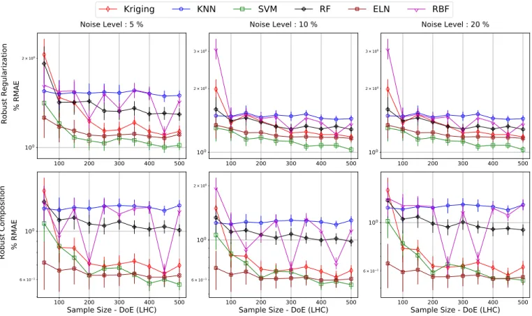
Fig. 6. Modeling accuracy of meta-model techniques on Ackley10Dwith three noise levels, two robustness strategies and ten training sample sizes.
100 200 300 400 500
2 × 100
3 × 100
% RMAE
Noise Level : 5 %
Robust Regularization
100 200 300 400 500
2 × 100
3 × 100
Noise Level : 10 %
100 200 300 400 500
2 × 100
3 × 100
Noise Level : 20 %
100 200 300 400 500
Sample Size - DoE (LHC)
2 × 100
3 × 100
% RMAE
Robust Composition
100 200 300 400 500
Sample Size - DoE (LHC)
2 × 100
100 200 300 400 500
Sample Size - DoE (LHC)
100 2 × 100
Kriging
KNN
SVM
RF
ELN
RBF
TABLE II
ALL36TEST CASES RESULTED FROM THE COMBINATION OF TWO META-MODELS,THREE LEVELS(NL),TWO ROBUST DEFINITIONS (ROBUST)AND FOUR FUNCTIONS. IN EACH TEST CASE,WE PICK THE BEST TWO META-MODELS IN TERMS OF AVERAGERMAE. GIVEN THE ALTERNATIVE HYPOTHESIS(Ha),THEMANNWHITNEYUTEST IS PERFORMED TO CHECK IF THE META-MODEL WITH HIGHEST AVERAGE ACCURACY IS SIGNIFICANTLY BETTER THAN THE SECOND BEST USING
α= 0.05. THE RESULTINGp-VALUES ARE PRESENTED.
Problem Robust NL Ha p-value
Ackley2D RR 5% KNN<SVM 0.425
Ackley2D RR 10% KNN<SVM 0.192
Ackley2D RR 20% KNN<SVM 0.012
Ackley2D RC 5% SVM<KNN 0.153
Ackley2D RC 10% SVM<KNN 0.136
Ackley2D RC 20% SVM<KNN 0.285
Branin2D RR 5% SVM<Kriging 0.395 Branin2D RR 10% Kriging<SVM 0.425 Branin2D RR 20% Kriging<SVM 0.153 Branin2D RC 5% Kriging<SVM 0.425 Branin2D RC 10% Kriging<SVM 0.425 Branin2D RC 20% Kriging<KNN 0.037
Ackley5D RR 5% SVM<ELN 0.010
Ackley5D RR 10% SVM<ELN 0.010
Ackley5D RR 20% SVM<KNN 0.010
Ackley5D RC 5% SVM<ELN 0.0001
Ackley5D RC 10% SVM<ELN 0.0001
Ackley5D RC 20% SVM<ELN 0.0001
Sphere5D RR 5% Kriging<ELN 0.0001 Sphere5D RR 10% Kriging<ELN 0.0001 Sphere5D RR 20% Kriging<ELN 0.0001 Sphere5D RC 5% Kriging<ELN 0.0001 Sphere5D RC 10% Kriging<RBFN 0.0001 Sphere5D RC 20% Kriging<ELN 0.002
Ackley10D RR 5% SVM<ELN 0.012
Ackley10D RR 10% SVM<ELN 0.008
Ackley10D RR 20% SVM<ELN 0.015
Ackley10D RC 5% ELN<SVM 0.285
Ackley10D RC 10% ELN<SVM 0.260
Ackley10D RC 20% ELN<SVM 0.120
Rastrigin10D RR 5% ELN<SVM 0.060 Rastrigin10D RR 10% ELN<SVM 0.060 Rastrigin10D RR 20% ELN<SVM 0.236 Rastrigin10D RC 5% ELN<SVM 0.037 Rastrigin10D RC 10% ELN<SVM 0.192 Rastrigin10D RC 20% ELN<SVM 0.052
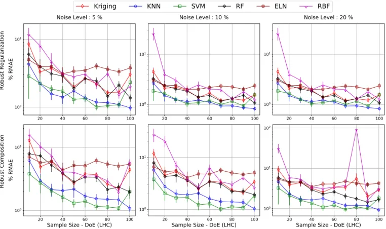
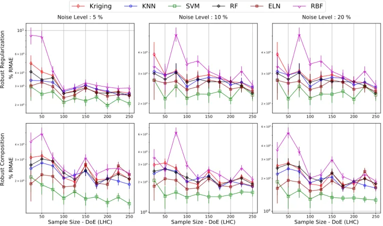
results on Ackley 2D. Similarly, figure 3 shows the accuracy on Branin 2D, figure 4 shows the accuracy on Ackley 5D, figure 5 presents the results for Sphere 5D, figure 6 presents the results concerning Ackley 10Dand lastly, figure 7 shows the results on Rastrigin 10D. It is important to state, that for each optimization case, we select the two best meta-models based on the measure of lowest RMAE, which is averaged over all values of training sizeN. We further perform Mann-Whitney U test to find if the meta-model with the lowest aver-age RMAE is significantly better than the other. The resulting
p-values are presented in Table II. In that table, the first col-umn reads the optimization problem under consideration, the second column presents the robustness strategies (i.e., RR for robust regularization and RC for robust composition), the third column reports the noise-level, the fourth column describes the two best meta-modeling techniques based on the lowest
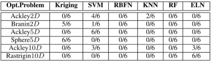
TABLE III
THE FREQUENCY OF META-MODELING TECHNIQUES ACHIEVING HIGHEST ACCURACY(I.E.,BASED ON THE VALUE OF LOWEST AVERAGERMAE)
FOR ALL SIX OPTIMIZATION PROBLEMS IS PRESENTED.
Opt.Problem Kriging SVM RBFN KNN RF ELN
Ackley2D 0/6 4/6 0/6 2/6 0/6 0/6
Branin2D 5/6 1/6 0/6 0/6 0/6 0/6
Ackley5D 0/6 6/6 0/6 0/6 0/6 0/6
Sphere5D 6/6 0/6 0/6 0/6 0/6 0/6
Ackley10D 0/6 3/6 0/6 0/6 0/6 3/6
Rastrigin10D 0/6 0/6 0/6 0/6 0/6 6/6
RMAE (i.e., alternative hypothesis) while the last column shows the p-value resulting from the Mann-Whitney U test. The frequencies of meta-modeling techniques achieving the highest accuracy for all optimization problems are presented in Table III. This Table follows the similar evaluation criteria i.e., lowest average RMAE.
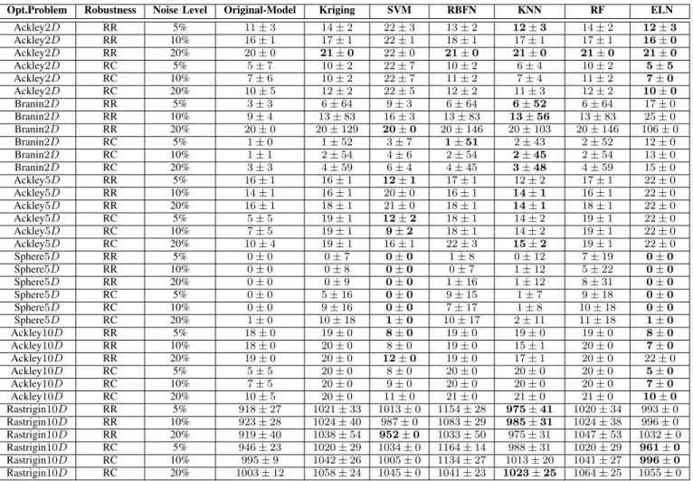
The results concerning the optimality ofR(x)for all thirty six cases are presented in Table IV. In this table, the first column reports the optimization problem, the second column reads the robustness scheme (i.e., RR for robust regularization and RC for robust composition), the third column presents the noise level, the fourth column shows the optimal value of
R(x), and all the next columns depict the optimal values of
R(x)proposed by all the meta-models.
Results from figures 2-7 suggest that robustness schemes and noise levels do not have much effect on the accu-racy of meta-models as we mostly observe similar patterns (i.e., RMAE curves) across rows and columns. Additionally, these figures depict that the Radial Basis Function Network (RBFN) has a lot of variance in prediction in all cases. Furthermore, these figures characterize that setting training size N = KD generally results in good modeling accuracy. HereK∈ {5,10,15,20,25,30,35,40,45,50} is a scalar and
D denotes the dimensions of the test problem. Hence, it can be observed that computational complexity of meta-models in this paper is a linear function of D. Table II shows that Kriging, Support Vector Machines (SVM) and Polynomial regression (ELN) achieve high accuracy in most test cases. In particular, Kriging performs well on Branin2Dand Sphere
5D. Polynomial regression (ELN) performs well on all5Dand
10D cases whereas SVM performs excellently in most cases for all of these dimensions. Table III shows that K-Nearest Neighbors (KNN) and Random Forest (RF) generally do not achieve high accuracy compared to other meta-models. Finally, Table IV shows that meta-models were able to find an optimal or near optimal solution in most cases except Rastrigin10D.
VI. CONCLUSIONS ANDOUTLOOK
TABLE IV
FINAL OPTIMAL FUNCTION VALUES FOR ALL THIRTY SIX CASES BY THE ORIGINAL MODEL AND ALL THE META-MODELS IS PRESENTED. FOR OPTIMIZATION, SLSQP [38]IS EMPLOYED ON THE ORIGINAL MODEL AND ALL THE META-MODELS. THE FUNCTION VALUES IN THE TABLE REPRESENT
THE MODE OF100RUNS ALONGSIDE THE STANDARD DEVIATION,BOTH ROUNDED OFF TO THE INTEGER REPRESENTATION. THE STARTING VALUE FOR SLSQPIS RANDOMLY SELECTED FROMLATINHYPER-CUBE SAMPLING FOR EACH SINGLE RUN. IN EACH CASE,META-MODELS WITH MOST OPTIMAL
FUNCTION VALUES(I.E.,BASED ON MODE AND IF TIED,BASED ON STANDARD DEVIATION)ARE HIGHLIGHTED.
Opt.Problem Robustness Noise Level Original-Model Kriging SVM RBFN KNN RF ELN
Ackley2D RR 5% 11±3 14±2 22±3 13±2 12±3 14±2 12±3
Ackley2D RR 10% 16±1 17±1 22±1 18±1 17±1 17±1 16±0
Ackley2D RR 20% 20±0 21±0 22±0 21±0 21±0 21±0 21±0
Ackley2D RC 5% 5±7 10±2 22±7 10±2 6±4 10±2 5±5
Ackley2D RC 10% 7±6 10±2 22±7 11±2 7±4 11±2 7±0
Ackley2D RC 20% 10±5 12±2 22±5 12±2 11±3 12±2 10±0
Branin2D RR 5% 3±3 6±64 9±3 6±64 6±52 6±64 17±0
Branin2D RR 10% 9±4 13±83 16±3 13±83 13±56 13±83 25±0
Branin2D RR 20% 20±0 20±129 20±0 20±146 20±103 20±146 106±0
Branin2D RC 5% 1±0 1±52 3±7 1±51 2±43 2±52 12±0
Branin2D RC 10% 1±1 2±54 4±6 2±54 2±45 2±54 13±0
Branin2D RC 20% 3±3 4±59 6±4 4±45 3±48 4±59 15±0
Ackley5D RR 5% 16±1 16±1 12±1 17±1 12±2 17±1 22±0
Ackley5D RR 10% 14±1 16±1 20±0 16±1 14±1 16±1 22±0
Ackley5D RR 20% 16±1 18±1 21±0 18±1 14±1 18±1 22±0
Ackley5D RC 5% 5±5 19±1 12±2 18±1 14±2 19±1 22±0
Ackley5D RC 10% 7±5 19±1 9±2 18±1 14±2 19±1 22±0
Ackley5D RC 20% 10±4 19±1 16±1 22±3 15±2 19±1 22±0
Sphere5D RR 5% 0±0 0±7 0±0 1±8 0±12 7±19 0±0
Sphere5D RR 10% 0±0 0±8 0±0 0±7 1±12 5±22 0±0
Sphere5D RR 20% 0±0 0±9 0±0 1±16 1±12 8±31 0±0
Sphere5D RC 5% 0±0 5±16 0±0 9±15 1±7 9±18 0±0
Sphere5D RC 10% 0±0 9±16 0±0 7±17 1±8 10±18 0±0
Sphere5D RC 20% 1±0 10±18 1±0 10±17 2±11 11±18 1±0
Ackley10D RR 5% 18±0 19±0 8±0 19±0 19±0 19±0 8±0
Ackley10D RR 10% 18±0 20±0 8±0 19±0 15±1 20±0 7±0
Ackley10D RR 20% 19±0 20±0 12±0 19±0 17±1 20±0 22±0
Ackley10D RC 5% 5±5 20±0 8±0 20±0 20±0 20±0 5±0
Ackley10D RC 10% 7±5 20±0 9±0 20±0 20±0 20±0 7±0
Ackley10D RC 20% 10±5 20±0 11±0 21±0 21±0 21±0 10±0
Rastrigin10D RR 5% 918±27 1021±33 1013±0 1154±28 975±41 1020±34 993±0
Rastrigin10D RR 10% 923±28 1024±40 987±0 1083±29 985±31 1024±38 996±0
Rastrigin10D RR 20% 919±40 1038±54 952±0 1033±50 975±31 1047±53 1032±0
Rastrigin10D RC 5% 946±23 1020±29 1034±0 1164±14 988±31 1020±29 961±0
Rastrigin10D RC 10% 995±9 1042±26 1005±0 1134±27 1013±20 1041±27 996±0
Rastrigin10D RC 20% 1003±12 1058±24 1045±0 1041±23 1023±25 1064±25 1055±0
if tied, based on standard deviation when compared with the original model. Additionally, in 12/36 cases, at least one meta-model achieves a better optimal value of the function than the original model following the similar evaluation criteria. In most of the remaining cases, at least one technique achieves near optimal function value when compared with the original model. From the results, in particular Tables II, III and figures 2-7, the authors conclude that Kriging, SVM and ELN provide a high modeling accuracy with limited training data in most cases. Additionally, these techniques find optimal or near optimal function values compared with the original model in most cases as presented in Table IV. The findings are a further validation of Kriging and Polynomial regression (i.e., in re-sponse surface approximation in structural engineering) as two of the most accurate meta-modeling techniques. The study also suggests SVM as a promising and competitive meta-model technique since it provides the highest modeling accuracy in most cases i.e., lowest average RMAE in 14/36 as presented in Table III and proposes near optimal solutions in most 5D
and10D cases in as shown in Table IV.
Future investigations are necessary to validate these tech-niques on more complex problems, i.e., multi-objective cases, higher dimensions, asymmetric noise and real-world engi-neering case studies etc. Further, it is important to model multiplicative noise and define other robustness strategies char-acterizing the practical nature of robust design optimization. Finally, there is a dire need to produce tutorial based cohesive work for engineers to adopt the meta-models in practical cases.
ACKNOWLEDGMENT
This research has received funding from the European Union’s Horizon 2020 research and innovation programme under grant agreement number 766186.
REFERENCES
[2] M. McIlhagga, P. Husbands, and R. Ives, “A comparison of search techniques on a wing-box optimisation problem,” inInternational Con-ference on Parallel Problem Solving from Nature, pp. 614–623, Springer, 1996.
[3] D. Wiesmann, U. Hammel, and T. B¨ack, “Robust design of multilayer optical coatings by means of evolutionary algorithms,”IEEE Transac-tions on Evolutionary Computation, vol. 2, no. 4, pp. 162–167, 1998. [4] J. W. Herrmann, “A genetic algorithm for minimax optimization
problems,” in Proceedings of the 1999 Congress on Evolutionary Computation-CEC99 (Cat. No. 99TH8406), vol. 2, pp. 1099–1103, IEEE, 1999.
[5] E. Kazancioglu, G. Wu, J. Ko, S. Bohac, Z. Filipi, S. J. Hu, D. Assanis, and K. Saitou, “Robust optimization of an automobile valvetrain using a multiobjective genetic algorithm,” inProceedings of DETC, vol. 3, pp. 2–6, 2003.
[6] H.-G. Beyer and B. Sendhoff, “Evolution strategies for robust op-timization,” in 2006 IEEE International Conference on Evolutionary Computation, pp. 1346–1353, IEEE, 2006.
[7] J. W. Kruisselbrinket al.,Evolution strategies for robust optimization. Leiden Institute of Advanced Computer Science (LIACS), Faculty of Science , 2012.
[8] F. Jurecka, Robust design optimization based on metamodeling tech-niques. PhD thesis, Technische Universit¨at M¨unchen, 2007.
[9] R. Jin, X. Du, and W. Chen, “The use of metamodeling techniques for optimization under uncertainty,” Structural and Multidisciplinary Optimization, vol. 25, no. 2, pp. 99–116, 2003.
[10] X. Du and W. Chen, “Methodology for managing the effect of un-certainty in simulation-based design,” AIAA journal, vol. 38, no. 8, pp. 1471–1478, 2000.
[11] H.-G. Beyer and B. Sendhoff, “Robust optimization–a comprehensive survey,” Computer methods in applied mechanics and engineering, vol. 196, no. 33-34, pp. 3190–3218, 2007.
[12] G. Taguchi, S. Konishi, and S. Konishi,Taguchi Methods: Orthogonal Arrays and Linear Graphs. Tools for Quality Engineering. American Supplier Institute Dearborn, MI, 1987.
[13] M. W. Trosset, “Taguchi and robust optimization,” tech. rep., 1996. [14] V. N. Nair, B. Abraham, J. MacKay, G. Box, R. N. Kacker, T. J.
Lorenzen, J. M. Lucas, R. H. Myers, G. G. Vining, J. A. Nelder,
et al., “Taguchi’s parameter design: a panel discussion,”Technometrics, vol. 34, no. 2, pp. 127–161, 1992.
[15] G. Box, S. Bisgaard, and C. Fung, “An explanation and critique of taguchi’s contributions to quality engineering,”Quality and reliability engineering international, vol. 4, no. 2, pp. 123–131, 1988.
[16] A. Ben-Tal, L. El Ghaoui, and A. Nemirovski, Robust optimization, vol. 28. Princeton University Press, 2009.
[17] Y. Carson and A. Maria, “Simulation optimization: methods and appli-cations,” inProceedings of the 29th conference on Winter simulation, pp. 118–126, IEEE Computer Society, 1997.
[18] D. H. Jung and B. C. Lee, “Development of a simple and efficient method for robust optimization,” International Journal for Numerical Methods in Engineering, vol. 53, no. 9, pp. 2201–2215, 2002. [19] W. Chen, J. K. Allen, K.-L. Tsui, and F. Mistree, “A procedure for
robust design: minimizing variations caused by noise factors and control factors,”Journal of mechanical design, vol. 118, no. 4, pp. 478–485, 1996.
[20] H. Agarwal, Reliability based design optimization: formulations and methodologies. University of Notre Dame, 2004.
[21] M. Papadrakakis, N. D. Lagaros, and V. Plevris, “Design optimization of steel structures considering uncertainties,” Engineering Structures, vol. 27, no. 9, pp. 1408–1418, 2005.
[22] X. Du and W. Chen, “Towards a better understanding of modeling feasibility robustness in engineering design,” Journal of Mechanical Design, vol. 122, no. 4, pp. 385–394, 2000.
[23] L. El Ghaoui and H. Lebret, “Robust solutions to least-squares problems with uncertain data,”SIAM Journal on matrix analysis and applications, vol. 18, no. 4, pp. 1035–1064, 1997.
[24] L. A. Schmit and B. Farshi, “Some approximation concepts for structural synthesis,”AIAA journal, vol. 12, no. 5, pp. 692–699, 1974.
[25] K. Svanberg, “The method of moving asymptotesa new method for structural optimization,”International journal for numerical methods in engineering, vol. 24, no. 2, pp. 359–373, 1987.
[26] V. Toropov, A. Filatov, and A. Polynkin, “Multiparameter structural op-timization using fem and multipoint explicit approximations,”Structural optimization, vol. 6, no. 1, pp. 7–14, 1993.
[27] W. Roux, N. Stander, and R. T. Haftka, “Response surface approxima-tions for structural optimization,”International Journal for Numerical Methods in Engineering, vol. 42, no. 3, pp. 517–534, 1998.
[28] G. E. Box and N. R. Draper, Empirical model-building and response surfaces. John Wiley & Sons, 1987.
[29] R. H. Myers, D. C. Montgomery, and C. M. Anderson-Cook,Response surface methodology: process and product optimization using designed experiments. John Wiley & Sons, 2016.
[30] J.-F. Barthelemy and R. T. Haftka, “Approximation concepts for opti-mum structural designa review,”Structural optimization, vol. 5, no. 3, pp. 129–144, 1993.
[31] T. J. Santner, B. J. Williams, W. Notz, and B. J. Williams,The design and analysis of computer experiments, vol. 1. Springer, 2003. [32] D. L¨onn, Ø. Fyllingen, and L. Nilssona, “An approach to robust
optimization of impact problems using random samples and meta-modelling,”International Journal of Impact Engineering, vol. 37, no. 6, pp. 723–734, 2010.
[33] V. Picheny and D. Ginsbourger, “Noisy kriging-based optimization methods: a unified implementation within the diceoptim package,”
Computational Statistics & Data Analysis, vol. 71, pp. 1035–1053, 2014. [34] K.-H. Lee and G.-J. Park, “A global robust optimization using kriging based approximation model,” JSME International Journal Series C Mechanical Systems, Machine Elements and Manufacturing, vol. 49, no. 3, pp. 779–788, 2006.
[35] T. W. Simpson, T. M. Mauery, J. J. Korte, and F. Mistree, “Kriging models for global approximation in simulation-based multidisciplinary design optimization,” AIAA journal, vol. 39, no. 12, pp. 2233–2241, 2001.
[36] K. Vanaja and R. Shobha Rani, “Design of experiments: concept and applications of plackett burman design,” Clinical research and regulatory affairs, vol. 24, no. 1, pp. 1–23, 2007.
[37] S. C. Ferreira, R. Bruns, H. Ferreira, G. Matos, J. David, G. Brandao, E. P. da Silva, L. Portugal, P. Dos Reis, A. Souza,et al., “Box-behnken design: an alternative for the optimization of analytical methods,”
Analytica chimica acta, vol. 597, no. 2, pp. 179–186, 2007.
[38] D. Kraft, “A software package for sequential quadratic programming,”