Vol 61, No 2 (2018)

TECHNICAL UNIVERSITY OF CLUJ-NAPOCA

ACTA TECHNICA NAPOCENSIS

Series: Applied Mathematics, Mechanics and Engineering Vol. 61, Issue II, June, 2018

MULTIPLE SOLUTIONS OF INTERPOLATION WITH SECOND

AND THIRD DEGREE BÉZIER POLYNOMIALS

Nicolae URSU-FISCHER, Diana Ioana POPESCU, Ioan RADU, Iuliana Fabiola MOHOLEA

Abstract: In this paper we study the problem of interpolation with Bézier functions, considering different conditions regarding the number of interpolation points, the degree of parametric interpolation parametric curves and the derivatives of these functions in the common points. The mathematical background about Bézier functions is presented, also some essential issues and the interpolation conditions that are required. The following three issues are studied and solved: interpolation with a second-degree Bézier function passing through three points, interpolation with multiple second-degree Bezier functions having the equal first-order derivatives in common points and, finally, interpolation with a third-degree Bézier function passing through four points. All deduced mathematical relations were programmed in C and various examples were presented in the paper. The work ends with a series of very useful conclusions.

Key words: interpolation, Bernstein’s polynomials, Bézier curves, two and three degree polynomials

1. INTRODUCTION

The problem of interpolation has been extensively studied, especially when polynomials are used. The interpolation with Lagrange polynomials is the most known, many engineering problems involving this type of interpolation [3], [13], [16] .

In the last fifty years, the use of some special functions, discovered by mathematicians and engineers, was widely spread, applied in computer aided design and implemented in actually software used in this domain.

The so-called Bézier [2] curves are in the attention of researchers for many years, mentioned in many books and scientific papers [4], [5], [6], [9], [10], [12], [14], [16], [17], each of which deals with some specific issues.

In the last years out team has studied many problems linked with the computer aided geometric design, using the Bézier, B-spline and NURBS functions.

In this paper our aim is to succeed in the study of interpolation with Bézier functions that accomplished some specified conditions, as concerns the number of interpolation points, the

degree of functions and the equality of first-degree derivatives in common points.

Further on it will be present a short mathematical background about the Bézier functions and the three specific issues that we have studied and solved.

2. BERNSTEIN POLINOMIALS AND BÉZIER CURVES

The Bernstein polynomials have the following expression [1], [2], [3], [4], [5]:

∑

=

− _∈

− =

Φ

n

k

k k n k n n

k t C t t t

0

, ( ) (1 ) , [0;1] (1)

and are used as a component part in Bézier functions:

∑

=

−

    

  

     

− =

     

=

n

k kP

P k k k n k

n B

B

y x t t C t

y t x t B

1

) 1 ( )

( ) ( )

( (2)

where (x0P, y0P), (x1P, y1P), …, (xkP, ykP), …,

(xn-1,P, yn-1,P), (xnP, ynP) are the coordinates of

the polygonal line vertices, named knots or control points. The polygonal line joining these points is named the control polygon.

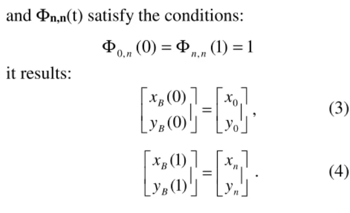
and Φ_n,n(t) satisfy the conditions: 1 ) 1 ( ) 0 ( _, ,

0 =Φ =

Φ n n n it results: , ) 0 ( ) 0 ( 0 0       =       y x y x B

B ₍₃₎

      =       n n B B y x y x ) 1 ( ) 1 (

. (4)

Therefore the Bézier curve starts at first point P0 of the control polygon and ends in the last

point Pn , without necessarily containing other

points of the control polygon.

Formula (2) may be written as follows:

+ − = Φ =

∑

, ( ) (1 )

)

(t t P C t P

B _n n

n

k

k n

k (5)

n n n n n n n n n

n t tP C t t P C t P

C − + + − +

+ − − − − 1 1 1 1 1

1_{(1 ) ... (1 )}

Calculating the first derivatives in the points that correspond to values t = 0 and t = 1 of the parameter t, it results:

) ( ) 1 ( , ( ) 0

( = ₁− ₀ ′ = − −₁

′ n n P P n B P P n

B (6)

3. SECOND-DEGREE BÉZIER FUNCTIONS THAT INTERPOLATE THREE POINTS

When the number of points is three and consequently the degree of Bézier functions is two, formula (2) may be written as:

] 1 ; 0 [ , ) 1 ( 2 ) 1 ( ) ( ) ( 2 2 2 1 1 2 0 0 ∈       + + −       + −       =       t t y x t t y x t y x t y t x P P P P P P B B (7)

The positions of points B₀=B(0)=P₀and

2 2 B(1) P

B = = are known

P B B

P B

B x x y y y

x

t=0, (0)= ₀ = ₀ , (0)= ₀ = ₀

P B B

P B

B x x y y y

x

t=1, (1)= ₂ = ₂ , (1)= ₂ = ₂

and a supplementary condition for the Bézier curve is added: it has to contain the third fixed point, noted B1 with the coordinates [x1B , y1B ].

Therefore, we have to find the position of the third (intermediate point) of the control

polygon, P0 – P1 – P2 , thus the corresponding

Bézier curve passes through the point B1. The

coordinates of vertex P1 will be computed from

the following linear equations:

2 1 2 1 1 1 2 1 0

1 x (1 t ) 2x (1 t )t x t

x_B= _B − + _P − + _B 2 1 2 1 1 1 2 1 0

1 y (1 t ) 2y (1 t )t y t

y_B= _B − + _P − + _B

The positions of the Bézier curve points in the plan Oxy depend on the positions of the three vertices of the control polygon and on the parameter t value, belonging to the interval [0;1]. The parameter value is noted with t1 .

It is easy to write the expressions of the unknown coordinates of point P1 :

) 1 ( 2 ) 1 ( 1 1 2 1 2 2 1 0 1 1 t t t x t x x

x_P B B B

− − − − = ) 1 ( 2 ) 1 ( 1 1 2 1 2 2 1 0 1 1 t t t y t y y

y_P B B B

− − − −

= (8)

We may conclude that there are different Bézier functions that interpolate points B0≡P0, B1 and B2≡P2, because we may consider any value for parameter t, the only condition being 0<t<1.

In figure 1 there are four second-degree Bézier curves, which achieve the desired interpolation, passing through three points, having different shapes. The difference is the value assigned to t1 parameter in each case: 0.2,

0.4, 0.6 and 0.8 . It is obvious that in each case the point P1 (the intermediate point of control

polygon) is located in different positions.

4. MULTIPLE SECOND-DEGREE

BÉZIER FUNCTIONS INTERPOLATING POINTS IN PLANE, HAVING EQUAL FIRST-ORDER DERIVATIVES IN COMMON POINTS

A number of n+1 points in the plan is considered, noted with P0 , P2 , . . . , P2n-2 , P2n.

If between each pair of points: P0 and P2 , P2

and P4 , P4 and P6 , . . . , P2n-4 and P2n-2 , P2n-2

and P2n there are n second-degree Bézier

curves with n-1 common points, the interpolation problem is solved. The positions of intermediate points of the control polygons with three vertices may be arbitrarily established and, as a consequence, in each of the n-1 common points the Bézier curves have different tangents. If our task is to obtain a Hermite type interpolation, it is necessary to impose the equality of first derivatives on both sides of common points, therefore the tangents to the adjacent curves have to fit. Imposing these conditions, we may obtain the unknown positions of intermediate points and the control polygons will ensure the existence of Bézier curves having equal first derivatives in common points.

Two adjacent Bézier curves have the following expressions:

2 2 1

2

2 2

2 2

1 2 2 2

) 1 ( 2

) 1 ( )

(

t P t t P

t P

t B

k k

k k

k k

+ − +

+ − =

−

− →

− → −

(9)

2 2 2 1

2

2 2

2 2 1 2 2

) 1 ( 2

) 1 ( ) (

t P t t P

t P t B

k k

k k

k k

+ +

+ → + →

+ − +

+ − =

(10)

Imposing the existence of the common tangent, it results:

) 0 ( )

1

( _{2 2 1 2 2}

2 1 2 2

2k− → k− → k =B k→ k+ → k+

B (11)

By combining (9), (10) and (11) we conclude:

1 , 1 ,

) (

2 1

, 0 2

1 2 1 2 2

1 2 2 1 2

− = +

=

= +

−

+ −

+ −

n k P

P P

P P P

k k

k

k k k

(12)

Knots P2k-1 and P2k+1 are placed in symmetric

positions with respect to the knot P2k (common

point of interpolation).

There are n intermediate points of the control polygons: P1 , P3 , … , P2n-3 and P2n-1

and the number of conditions is n-1. The problem will be solved by considering imposed values to the coordinates of one point, e.g. of point P1 .

Relations (13) will be used to compute the coordinates of points P3, … , P2n-3 and P2n-1.

The above explained procedure was used to perform the interpolations presented in figures 2, 3, 4 and 5.

3 2 2 2 1 2 5 2 4 2 3 2

5 6 7 3 4 5 1 2 3

2 ,

2 ,. ..

, 2

, 2

, 2

− − −

− −

− = − = −

− = −

= −

=

n n n

n r n

n P P P P P

P

P P P P P P P P P

(13)

Fig. 2. Imposed coordinates of P1[20 ; 20]

Fig. 4. Imposed coordinates of P1[20 ; 80]

Fig. 5. Imposed coordinates of P1[80 ; 80]

Fig. 6. Superposed diagrams from figures 2 to 5 The number of points to interpolate was six and the shape of diagrams differs because the position of point P1 is changed from figure to

figure. One may observe the existence of

common tangents in the points 2, 4, 6 and 8, the Hermite type interpolation being performed.

Fig. 7. Other four different positions of point P1

In figure 6 are shown the superposed diagrams, corresponding to figures 2, 3, 4 and 5. In figure 7 other four diagrams are presented, obtained considering other four different positions of point P1.

5. INTERPOLATION USING THIRD- DEGREE BÉZIER FUNCTIONS THAT PASS THROUGH FOUR POINTS IN PLAN

If the degree of Bézier function is three, the control polygon has four knots (vertices), the first and the last coincide with the first point of the Bézier curve (for t=0) and with the final point (obtained for t=1).

The interpolation problem will be solved considering that the Bezier curve has to contain two specified points in the plan, denoted by B1

and B2, with known coordinates: [x1B ,y1B ]

respectively [ x2B , y2B].

In this case, formula (2) becomes:

] 1 ; 0 [

, )

1 ( )

( )

( 3

0

3 3

∈

    

  

     

− =

   

 

∑

=

−

t

y x t t C t

y t x

k kP

P k k k k

B B

(14)

and developing we obtain:

P P

P P

B

x t x t t

x t t x

t t

x

3 3 2 2

1 2 0

3

) 1 ( 3

) 1 ( 3 )

1 ( ) (

+ −

+

+ −

+ −

=

(15)

P P

P P

B

y t y t t

y t t y

t t

y

3 3 2 2

1 2 0

3

) 1 ( 3

) 1 ( 3 )

1 ( ) (

+ −

+

+ −

+ −

=

After imposing the conditions (the curve must pass through two points B2 and B3), the

following two relations will result, involving abscissas: 1 0 , ) 1 ( 3 ) 1 ( 3 ) 1 ( ) ( 1 3 3 1 2 2 1 1 1 1 2 1 0 3 1 1 1 < < + − + + − + − = = t x t x t t x t t x t x t x P P P P B B 1 , ) 1 ( 3 ) 1 ( 3 ) 1 ( ) ( 2 1 3 3 2 2 2 2 2 1 2 2 2 0 3 2 2 2 < < + − + + − + − = = t t x t x t t x t t x t x t x P P P P B B

and other two for ordinates:

1 0 , ) 1 ( 3 ) 1 ( 3 ) 1 ( ) ( 1 3 3 1 2 2 1 1 1 1 2 1 0 3 1 1 1 < < + − + + − + − = = t y t y t t y t t y t y t y P P P P B B 1 , ) 1 ( 3 ) 1 ( 3 ) 1 ( ) ( 2 1 3 3 2 2 2 2 2 1 2 2 2 0 3 2 2 2 < < + − + + − + − = = t t y t y t t y t t y t y t y P P P P B B

Two systems of linear equations were obtained, each of them having two unknowns: the coordinates of the control polygon vertices P1 and P2 :

P P B P P x t x t x x t t x t t 3 3 1 0 3 1 1 2 2 1 1 1 1 2 1 ) 1 ( ) 1 ( 3 ) 1 ( 3 − − − − = − + − P P B P P x t x t x x t t x t t 3 3 2 0 3 2 2 2 2 2 2 1 2 2 2 ) 1 ( ) 1 ( 3 ) 1 ( 3 − − − − = − + − (17) P P B P P y t y t y y t t y t t 3 3 1 0 3 1 1 2 2 1 1 1 1 2 1 ) 1 ( ) 1 ( 3 ) 1 ( 3 − − − − = − + − P P B P P y t y t y y t t y t t 3 3 2 0 3 2 2 2 2 2 2 1 2 2 2 ) 1 ( ) 1 ( 3 ) 1 ( 3 − − − − = − + − (18)

Both systems are compatible, the unknowns can be calculated, because the discriminant of the system of equations is different from zero, it being positive: 0 ) t t ( ) t 1 ( ) t 1 ( t t

9 _{1 2} − ₁ − _{2 2} − ₁ >

=

∆ .

As we notice, the values of parameters t1

and t2 intervene in the expressions of knots P1

and P2 coordinates, thus the shapes of the

Bézier curves (determined by the control polygon) are different, depending on the considered values for t1 and t2 , but all of

them have the property to interpolate the four imposed points.

In figures 8 to 13 six Bézier interpolation curves are shown, that pass through four given points of coordinates: B0[50; 80], B1[80; 120],

B2[150; 145] and B3[300; 50], having different

shapes, depending on the assumed values for parameters t1 and t2.

Fig. 8. The coordinates of vertices P1[86.11;158.61] and P2 [197.22;184.72]

Fig. 9. The coordinates of vertices P1 [-19.44;56.11] and P2 [202.78;261.39]

Fig.11. The coordinates of vertices P1[223.45;288.46] and P2 [-66.28;237.16]

Fig.12. The coordinates of vertices P1[559.26;-369.81] and P2 [-345.06;487.47]

Fig.13. The coordinates of vertices P1[147.22;-3.70] and P2 [-47.22;310.20]

In figure 14 are shown seven interpolation Bézier functions of third-degree that pass through four points. Four of these curves are those presented in figures 8 to 11.

Fig.14. Superposed diagrams corresponding to seven interpolation Bézier functions, obtained for different

values of parameters t1 and t2 6. CONCLUSIONS

The purpose of this paper was to present some important problems regarding the interpolation with low degrees Bézier curves.

Despite the fact that problems of interpolation with Bézier, B-spline and NURBS curves have been extensively studied during the last time, there are still some particular problems - we dare to see of great interest in this field – which have not been studied at all or have been insufficiently studied.

Three important issues have been in our attention:

- the interpolation with a single Bézier curve of second-degree, considering three points of interpolation;

- the interpolation with multiple adjacent Bézier curves of second-degree, having the first derivatives equal in the common points;

- the interpolation with a single third-degree Bézier curve that interpolates four points.

To solve these issues, all necessary mathematical aspects have been elucidated. The deduced formulas were programmed in C language [11], [15] and many examples are presented in the paper for each case.

and supplementary, in case of Hermite interpolation, to have imposed values of first derivatives in the interpolating points.

In the case of interpolation with Bézier functions, the situation is changed: we may obtain different solutions (different curves) that fulfill the imposed conditions. The examples presented above - and one may examine figures 1, 6, 7 and 14 - show that different curves pass through the imposed points and, in some cases, also satisfy supplementary conditions about the derivative values in interpolating points or in the common interpolating points, when adjacent curves exist.

In each studied case the explanations are the same: the number of condition to be imposed is less than the number of unknowns.

The supplementary conditions may be imposed in different manners: by choosing values of parameters defining the positions of points on the Bézier curves, by choosing positions for some points of control polygon, etc.

Obviously, the possibility to obtain multiple solutions for the interpolation problem is an advantage when we choose a desired interpolation curve.

7. REFERENCES

[1] Bender, M., Brill, M., Computergrafik. Ein anwendungsorientiertes Lehrbuch, Carl

Hansen Verlag, München, 2003, 516 pp., ISBN 3-446-22150-6

[2] Bézier, P., Mathématiques et CAO. Courbes et surfaces, volume 4, Ed. Hermes, Paris,

1987

[3] Engeln-Müllges, Gisela, Uhlig, F.,

Numerical Algorithms with C, Springer,

New York, 1996, 596 pp., ISBN 3-540-60530-4

[4] Farin, G. E., Curves and Surfaces for Computer Aided Geometric Design. A Practical Guide, Academic Press, San

Diego, sec. ed., 1990, 444 pp., ISBN 0-12-249051-7

[5] Farin, G., Hoschek, J., Kim, M.-S. (eds.),

Handbook of Computer Aided Geometric

Design, Elsevier, Amsterdam, 2002, 820 pp.,

ISBN 0-444-51104-0

[6] Foley, J. D., van Dam, A., Hughes, J. F.,

Computer Graphics, Principles and Practice, 2/e in C, Addison-Wesley, 1996,

1200 pp.

[7] Forrest, A. R., Interactive interpolation and approximation by Bézier polynomials, The

Computer Journal, 1972, Vol. 15, No. 1, pp. 71-79

[8] Lu, L., Sample-based polynomial appro-ximation of rational Bézier curves, Journal

of Computational and Applied Mathematics, 2011, Vol. 235, pp. 1557-1563

[9] Lyche, T., Schumacher, L. L. (ed.),

Mathematical Methods in Computer Aided Geometric Design, Academic Press, San

Diego, 1989, 611 pp., ISBN 0-12-460515-X [10] Nischwitz, A., Haberäcker, P., Masterkurs Computergrafik und Bildverarbeitung,

Friedrich Viewig & Sohn Verlag, Wiesbaden, 2004, 860 pp., ISBN 3-528-05874-9

[11] Popescu, D. I, Programare în limbajul C

(Programming in C- in Romanian), Ed. "DSG Press", Dej, 1999, 288 pp., ISBN 973-98621-4-4

[12] Popescu, D. I., Aplicaţii cu SolidWorks. CAD în ingineria mecanică (Applications

with SolidWorks. CAD in Mechanical Engineering – in Romanian), Editura Dacia, Cluj-Napoca, 2003, 191 pp., ISBN 973-35-1728-3

[13] Pozrikidis, C., Numerical Computation in Science and Engineering, University Press,

Oxford, 1998, 640 pp., ISBN 0-19-511253-9 [14] Rogers, D. F., Adams, J. A., Mathematical Elements for Computer Graphics, McGraw

Hill, Boston, sec. ed., 1990, 611 pp., ISBN 0-07-053530-2

[15] Ursu-Fischer, N., Ursu, M., Programare cu C în inginerie (Programming with C in

Engineering – in Romanian), Casa Cărţii de Ştiinţă, Cluj-Napoca, 2001, 405 pp., ISBN

973-686-227-5

[16] Ursu-Fischer, N., Ursu, M., Metode numerice în tehnică şi programe în C/C++

Casa Cărţii de Ştiinţă, Cluj-Napoca, 2003,

288 pp., ISBN 973-686-464-2

[17] Xiao, G., Xu, X., Study on Bézier curve variable step-length algorithm, Physics

Procedia, 2012, Vol. 25, pp. 1781-1786.

Asupra unor soluţii multiple de interpolare cu polinoame Bézier de gradul doi şi trei

Rezumat: În această lucrare este studiată problema interpolării cu funcţii Bézier, considerând diferite condiţii privind

numărul punctelor de interpolare, gradul curbelor parametrice de interpolare precum şi derivatele acestor funcţii în

punctele comune.

Sunt prezentate câteva probleme esenţiale privind funcţiile Bézier, precum şi condiţiile de interpolare care se impun.

Sunt studiate şi rezolvate următoarele trei probleme: interpolarea cu o funcţie Bézier de gradul doi care trece prin trei

puncte, interpolarea cu mai multe funcţii Bézier de gradul doi, successive, în punctele comune având tangente identice şi interpolarea cu funcţii Bézier de gradul trei care trec prin patru puncte.

Toate relaţiile matematice au fost programate în cadrul unui program C, pe baza căruia au fost realizate o serie de

exemple care sunt prezentate în lucrare.

Lucrarea se încheie cu o serie de concluzii foarte utile.

Nicolae URSU-FISCHER, Prof. dr. eng. math., Technical University of Cluj-Napoca, Department of Mechanical Systems Engineering, E-mail: [email protected], Phone: 0264-401659

Diana IOANA POPESCU, Prof. dr. eng., Technical University of Cluj-Napoca, Department of Mechanical Systems Engineering, E-mail: [email protected], Phone: 0264-401783 Ioan RADU, Prof. dr. eng., “Aurel Vlaicu” University Arad, Faculty of Engineering, Department

of Automation, Industrial engineering, Textile production and Transport, E-mail: [email protected], Phone: 0257-283010