Practical, Real-time, Full Duplex Wireless
Mayank Jain
†1, Jung Il Choi
†1, Tae Min Kim
1, Dinesh Bharadia
1, Siddharth Seth
1,
Kannan Srinivasan
2, Philip Levis
1, Sachin Katti
1, Prasun Sinha
3 1Stanford University 2
The University of Texas at Austin 3
The Ohio State University
California, USA Texas, USA Ohio, USA
{mayjain, jungilchoi, kimtm, dineshb, sidseth}@stanford.edu,
[email protected], [email protected],
[email protected], [email protected]
†
Co-primary authors
Abstract
This paper presents a full duplex radio design using signal inversion and adaptive cancellation. Signal inversion uses a simple design based on a balanced/unbalanced (Balun) transformer. This new de-sign, unlike prior work, supports wideband and high power sys-tems. In theory, this new design has no limitation on bandwidth or power. In practice, we find that the signal inversion technique alone can cancel at least 45dB across a 40MHz bandwidth. Further, com-bining signal inversion cancellation with cancellation in the digital domain can reduce self-interference by up to 73dB for a 10MHz OFDM signal.
This paper also presents a full duplex medium access control (MAC) design and evaluates it using a testbed of 5 prototype full duplex nodes. Full duplex reduces packet losses due to hidden ter-minals by up to 88%. Full duplex also mitigates unfair channel allocation in AP-based networks, increasing fairness from 0.85 to 0.98 while improving downlink throughput by 110% and uplink throughput by 15%. These experimental results show that a re-design of the wireless network stack to exploit full duplex capabil-ity can result in significant improvements in network performance.
Categories and Subject Descriptors
C.2.1 [Computer-Communication Networks]: Network Archi-tecture and Design—Wireless communication
General Terms
Design, Performance, Reliability
Keywords
Full-duplex wireless
1.
INTRODUCTION
Wireless radios today are generally half duplex. On a single channel, they can either transmit or receive, but not both
simultane-Permission to make digital or hard copies of all or part of this work for personal or classroom use is granted without fee provided that copies are not made or distributed for profit or commercial advantage and that copies bear this notice and the full citation on the first page. To copy otherwise, to republish, to post on servers or to redistribute to lists, requires prior specific permission and/or a fee.
MobiCom’11,September 19–23, 2011, Las Vegas, Nevada, USA. Copyright 2011 ACM 978-1-4503-0492-4/11/09 ...$10.00.
ously. The inability to do both simultaneously is the root of many of the open problems in wireless today, such as media access con-trol and bitrate adaptation. A full duplex radio has the potential to completely reconsider how we design and build wireless networks. The possible benefits of full duplex wireless have recently led researchers to explore how one might build such a device [4]. The basic challenge is reducing self interference. If a node cannot hear its own signal, then its own transmissions will not interfere with other packets: it can simultaneously transmit and receive.
Well known digital and analog techniques, even when combined together, are not sufficient to cancel self-interference sufficiently for full duplex [4]. Some analog cancellation techniques use noise canceling chips to subtract the self transmission signal (the “noise”) from the received signal [12]. Digital cancellation, used in CS-MA/CN, optical networks and proposals for full duplex operation, subtracts self-interference in the digital domain, after the receiver has converted the baseband signal to digital samples [14, 6, 3].
Motivated by these limitations, recent work has explored antenna placement as an additional cancellation technique. Antenna separa-tion uses the fact that the distance between the transmit and receive antennas naturally reduces self-interference due to signal attenu-ation [5]. However, we would need impractically large distances between the TX and RX antennas to obtain enough reduction to make full duplex possible with only antenna separation. To further cancel self-interference, Choi et al. propose an additional tech-nique, called antenna cancellation [4]. Antenna cancellation, when combined with the other mechanisms, allows full duplex operation: Choi et al. evaluate working 802.15.4 (1mW) full duplex proto-types which are close to (within 8%) an ideal full duplex system.
Although promising, antenna cancellation-based designs have three major limitations. The first is that they require three antennas: two transmit, and one receive. Full duplex doubles throughput, but with three antennas a MIMO system can triple throughput, so from a raw performance standpoint antenna cancellation is unattractive. Furthermore, having two transmit antennas creates slight null re-gions of destructive interference in the far field. The second lim-itation is a “bandwidth constraint,” a theoretical limit which pre-vents supporting wideband signals such as WiFi. Finally, Choi et al.’s design introduces a third, practical limitation: it requires man-ual tuning. While manman-ual tuning is sufficient for lab experiments demonstrating a proof of concept, it leaves open the question of whether it is possible to build a full duplex system that can auto-matically adapt to realistic environments.
Baseband Mapping 0011100 Transmit Bits RF Mixer Baseband Signal RF TX Signal TX Carrier Frequency Baseband Samples Digital to Analog Converter (DAC) Baseband Demapping 0011100 Receive Bits RF Mixer Baseband Signal RF RXSignal RX Carrier Frequency Baseband Samples Analog to Digital Converter (ADC)
Figure 1: Simplified block diagram of an RF Receiver
The first contribution of this paper is a full duplex radio design that addresses all three limitations. It proposes a novel mechanism, balun cancellation, that uses signal inversion, through a balun (bal-anced/unbalanced) circuit. Balun cancellation has no bandwidth constraint: it can in theory support arbitrary bandwidths and can-cel arbitrarily high transmit powers. Balun cancan-cellation requires only two antennas, one transmit and one receive. Furthermore, this paper presents a tuning algorithm that allows a balun-based radio design to quickly, accurately, and automatically adapt the full du-plex circuitry to cancel the primary self-interference component.
The second contribution is the implementation and evaluation of the balun cancellation design as well as a full duplex MAC proto-col. It explores how and where practice differs from theory, exam-ining the engineering challenges that arise in making full duplex practical. For example, while a balun can in theory provide perfect cancellation, this assumes that the balun has a flat frequency re-sponse: if not flat, the inverted signal might differ slightly from the transmitted signal. These results indicate possible future challenges in large scale full duplex radio production.
We evaluate the design in two ways. The first is using a tightly controlled channel sounder1to demonstrate the limits of the exist-ing circuitry at the physical layer. We find that well-tuned balun cancellation circuit built from commodity components can cancel over 45dB across a 40MHz bandwidth. Combined with digital cancellation, this allows a full duplex radio to cancel up to 73dB of self-interference: consequently full duplex 802.11n devices are possible with a reasonable separation between TX and RX anten-nas. The second evaluation uses a 5-node WARP software radio testbed to quantify the link-layer benefits of a full duplex MAC layer based on the Contraflow design [13].
2.
RADIO DESIGN AND FULL DUPLEX
This section provides background on the basics of radio design as well as full duplex. It explains the basic challenges in building a full duplex radio, the existing techniques for doing so, and the limitations of those techniques.2.1
Radio Design
Figure 1 shows the basic design of a modern radio receiver. We walk through these details because the underlying data representa-tions determine how and when a full duplex radio can cancel sig-nals. We use channel 1 of 802.11b as a running example to ground the concepts in concrete numbers.
A wireless signal occupies a bandwidth, a range of frequen-cies. 802.11b channels, for example, are 22MHz wide. Chan-nel 1 of 802.11b is centered at 2.412GHz: it spans 2.401GHz to 2.423GHz. The signal transmitted and received at this frequency range is called theRF (Radio Frequency) signal. Because digitally sampling a 2.4GHz signal would require very high speed sampling at the Nyquist frequency of 4.8GHz, radios downconvert a RF
sig-1
These channel sounders are wideband (∼240MHz) radios used for RF profiling, programmed to generate a single wideband pilot pattern for measuring the channel.
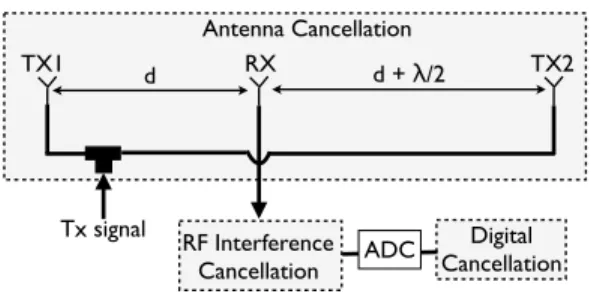
Digital Cancellation d d + λ/2 TX1 RX TX2 ADC RF Interference Cancellation Antenna Cancellation Tx signal
Figure 2: Block diagram of existing full duplex design with three cancellation techniques.
nal to abaseband signalcentered around0Hz. The baseband signal of 802.11b occupies -11 to 11 MHz. Downconverting allows the ra-dio to use a much lower speed analog to digital converter (ADC): the 22MHz baseband signal needs an ADC operating at or slightly above the Nyquist rate of 44 MHz. Commodity WiFi cards typi-cally use 8-bit samples, though some software radios can provide 12 bit resolution.
To transmit a packet, a radio generates digital samples for the desired waveform, converts them to a baseband signal with a digital to analog converter (DAC) and upconverts the baseband to RF. To receive a packet, a radio downconverts an RF signal to a baseband signal, then samples the baseband with an ADC to generate digital samples.
2.2
Cancellation
The goal of a full duplex radio is to transmit and receive simul-taneously. The problem is that a node hears not only the signal it wants to receive, but also the signal it is transmitting. By cancel-ing this self-interference from what it receives, a full duplex node can in theory decode a received signal. This cancellation is hard, however, because the self-interference can be millions to billions of times stronger (60-90 dB) than a received signal. For example, a radio with a transmit power of 0dBm and a noise floor of approxi-mately -90dBm needs to cancel nearly 95dB of self-interference to ensure that its own transmissions do not disrupt reception.
There are existing digital and analog techniques to cancel inter-ference. Digital cancellation operates on digital samples. If a full duplex radio has a good estimate of the phase and amplitude of its transmitted signal at the receive antenna, it can generate the dig-ital samples for its transmitted signal and subtract them from its received samples. Digital cancellation, while helpful, is by itself insufficient: current systems in the research literature cancel up to 20-25 dB [8, 7]. The limitation is that ADCs have a limited dy-namic range: since self-interference is extremely strong, an ADC can quantize away the received signal, making it unrecoverable af-ter digital sampling.
Analog cancellation uses knowledge of the transmission to can-cel self-interference in the RF signal, before it is digitized. One approach to analog cancellation uses a second transmit chain to create an analog cancellation signal from a digital estimate of the self-interference [5], canceling≈33dB of self-interference over a 625kHz bandwidth signal. Another approach uses techniques sim-ilar to noise-canceling headphones [12]. The self-interference sig-nal is the “noise” which a circuit – the QHx220 chip [11] – sub-tracts from the received signal. The QHx220 can cancel 20-25 dB for a 10MHz bandwidth signal but it introduces numerous com-plications, such as non-linearities and distortions, which compli-cate digital cancellation significantly. We examine these limitations more deeply in Section 5.1, but the overall result is that this
ap-proach cannot provide more than 25 dB of cancellation and cannot be combined with digital cancellation: it is therefore insufficient for full duplex.
2.3
Full Duplex
Motivated by the above limitations, recent work has proposed antenna placement techniques [4, 5]. The state of the art in full du-plex operates on narrowband 5MHz signals with a transmit power of 0dBm (1mW) [4]. The design achieves this result by augmenting the digital and analog cancellation schemes described above with a novel form of cancellation called “antenna” cancellation. Figure 2 shows a block diagram of this design. The separation between the receive and transmit antennas attenuates the self-interference signal [5], but this antenna separation is not enough. The key idea behind antenna cancellation is to use a second transmit an-tenna and place it such that the two transmit signals interfere de-structively at the receive antenna. It achieves this by having one-half wavelength distance offset between the two transmit anten-nas. The resulting destructive interference cancels 20-30dB of self-interference. Combined with the analog and digital cancellation de-scribed above, the design is able to cancel 50-60dB of self-interference, which is sufficient to operate a full duplex 802.15.4 radio.
This design, while a breakthrough, has both fundamental and practical limitations. The first limitation is fundamental and re-lates to the bandwidth of the transmitted signal. Antenna cancel-lation ensures that only the signal at the center frequency is per-fectly inverted in phase at the receive antenna and thus cancelled fully. However, as a signal moves further away from the center frequency, the phase offset of two versions from the transmit an-tennas shifts away from perfect inversion and so the two do not cancel completely. Correspondingly, antenna cancellation perfor-mance degrades as the bandwidth of the signal to cancel increases. In practice, this means antenna cancellation cannot cancel an 802.11b signal by more than 30dB: Choi et al. note that it may be just barely possible to build a full duplex 802.11b node [4]. Widen-ing the signal to 40MHz (e.g., 802.11n) precludes full duplex at WiFi transmit powers.
Furthermore, as the cancellation is highly frequency selective, modulation approaches such as OFDM which break a bandwidth into many smaller parallel channels will perform even more poorly. Due to frequency selectivity, different subcarriers will experience drastically different self-interference. Hence cancellation suffers for wideband OFDM systems that do not adapt on a per subcar-rier basis. As WiFi and other wireless technologies move towards OFDM (802.11n and 802.11g use it) due to its technical advan-tages, antenna cancellation will encounter serious challenges.
Antenna cancellation’s second limitation is requiring three an-tennas. Full duplex at most doubles throughput. But with three antennas, a 3x3 MIMO array can theoretically triple throughput. This comparison suggests it may be better to just use MIMO and sacrifice some portion of the available capacity for other useful link layer primitives such as RTS/CTS. Furthermore, having two trans-mit antennas creates slight null regions of destructive interference in the far field.
The third limitation relates to the details of Choi et al.’s design. The full duplex radio requires manually tuning the phase and am-plitude of the second transmit antenna to maximize cancellation at the receive antenna. While manual tuning is sufficient for a lab proof-of-concept, it is an open question whether it is technically feasible to design a circuit that automatically tunes itself in a dy-namic environment.
Digital Interference Cancellation
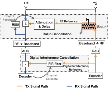
TX RX Attenuation & Delay RF ! Baseband ADC Baseband ! RF DAC Encoder Decoder Digital Interference Reference Balun Cancellation
TX Signal Path RX Signal Path
RF Reference Σ FIR filter -RSSI Control Feedback Channel Estimate Balun
Figure 3: Block diagram of full duplex system. The ideal can-cellation setup uses passive, high precision components for at-tenuation and delay adjustment.
3.
DESIGN
In this section we describe the design of a full duplex system radio that requires only 2 antennas and RF frontends, has no band-width constraint, and automatically tunes its self-interference can-cellation in response to changing channel conditions.
3.1
Eliminating the Bandwidth Constraint
The design is based on a simple observation: any radio that inverts a signal through adjusting phase will always encounter a bandwidth constraint that bounds its maximum cancellation. To cancel beyond this bound, a radio needs to obtain the perfect in-verseof a signal, i.e., a signal which is the perfect negative of the transmitted signal at all instants. Combining this inverse with the transmitted signal can in theory completely cancel self-interference. All a radio needs is to invert a signal without adjusting its phase. Luckily, there is a component that does exactly that: a balanced/un-balanced (balun) transformer. Baluns are a common component in RF, audio and video circuits for converting back and forth between single-ended signals – single-wire signals with a common ground – and differential signals – two-wire signals with opposite polarity. For example, converting a single-ended signal on a co-axial cable to a differential signal for transmission on a twisted pair cable (such as Ethernet), or vice-versa, uses a balun to take the signal as input and output the signal and its inverse.The key insight of this paper is that one can use a balun in a completely new way, to obtain the inverse of a self-interference signal and use the inverted signal to cancel the interference. Fig-ure 3 shows a 2-antenna full duplex radio design that uses a balun. The transmit antenna transmits the positive signal. To cancel self-interference, the radio combines the negative signal with its re-ceived signal after adjusting the delay and attenuation of the nega-tive signal to match the self-interference.
We call this techniquebalun passive cancellationsince we ide-ally use high precision passive components to realize the variable attenuation and delay in the cancellation path. While balun cancel-lation can in theory cancel perfectly, there are of course practical limitations. For example, the transmitted signal on the air expe-riences attenuation and delay. To obtain perfect cancellation the radio must apply identical attenuation and delay to the inverted
sig-240 MHz TX @2.4GHz RX Variable Attenuator Balun Variable Delay Line ! 20dB Attenuator Self-interference path Cancellation Path
Figure 4: Wired setup to measure the cancellation performance of signal inversion vs phase offset. The phase offset experiment uses an RF splitter instead of a balun to split the signal.
2300 2350 2400 2450 2500 2550 2600 −110 −100 −90 −80 −70 −60 Frequency in Mhz Received signal (dBm) 2300 2350 2400 2450 2500 2550 2600 −110 −100 −90 −80 −70 −60 Balun Phase Offset
Figure 5: Cancellation of the self-interference signal with the balun vs with phase offset. The received signal is -49dBm with-out any cancellation. Using a balun gives a flatter cancellation response.
nal before combining it, which may be hard to achieve in practice. Moreover, the balun may have engineering imperfections, such as leakage or a non-flat frequency response. The rest of this section examines these practical concerns and how to solve them.
3.2
Balun Benefits
To understand the practical benefits and limitations of inverting a signal with a balun, compared to inverting it with a phase offset, we conduct a tightly controlled RF experiment. Figure 4 shows the experimental setup. We program a signal generator to generate a wideband 240MHz chirp with a center frequency of 2.45GHz. This signal goes over two wires. The first wire is an ideal self-interference path and has a 20dB attenuator representing the an-tenna separation. The second wire goes through a cancellation path, consisting of a variable attenuator and variable delay element that can be controlled to modify the cancellation path signal to match the self-interference. The combination of the two signals feeds into a signal receiver. The variable delay line and attenuator in this ex-periment are manually tunable passive devices which allow for a high degree of precision.
We simulate antenna cancellation by making the cancellation path one half of a wavelength longer than the self-interference path. An RF combiner adds the two signals on the received side to mea-sure the canceled signal. The balun setup, on the other hand, uses a balun to split the transmit signal, and uses wires of the same length for the self-interference and cancellation paths. In both cases, the passive delay line and attenuator provide fine-grained control to match phase and amplitude for the interference and cancellation paths to maximize cancellation.
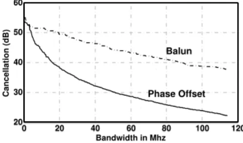
Figure 5 shows the results. Using a phase-offset signal can-cels well over a narrow bandwidth, but is very limited in canceling wideband signals. Phase offset cancellation can cancel 50dB for a 5MHz signal, but only provide 25dB of cancellation for a 100MHz
0 20 40 60 80 100 120 20 30 40 50 60 Bandwidth in Mhz Cancellation (dB) 0 20 40 60 80 100 120 20 30 40 50 60 Phase Offset Balun
Figure 6: Cancellation performance with increasing signal bandwidth when using the balun method vs using phase offset cancellation.
signal. In comparison, the balun based circuit provides a good de-gree of cancellation over a much wider bandwidth. For example, balun based cancellation would provide 52dB of cancellation for a 5MHz signal and 40dB of cancellation for a 100MHz signal.
Balun cancellation is not perfect across the entire band. The key reason is that the balun circuit is not frequency flat, i.e., different parts of the band are inverted with different amplitudes. Conse-quently applying a single attenuation and delay factor to the in-verted signal will not cancel the transmitted signal perfectly: this is a simple instance of real-world engineering tolerances limiting theory. Based on Figure 5, we can obtain the best possible cancel-lation with balun and phase-offset cancelcancel-lation for a given signal bandwidth. Figure 6 shows the best cancellation achieved using each method for signals of varying bandwidths.
3.3
Auto-tuning
The results in Figure 6 show that, if the phase and amplitude of the inverted signal are set correctly, balun cancellation can have impressive results across a wide bandwidth. This raises a sim-ple follow-on question. Is it possible to automatically adjust the phase and amplitude, thereby self-tuning cancellation in response to channel changes? In this section we describe an algorithm that can accurately and quickly self-tune a cancellation circuit.
The basic approach is to estimate the attenuation and delay of the self-interference signal and match the inverse signal appropriately. Ideally, the auto-tuning algorithm would adjust the attenuation and delay such that the residual energy after balun cancellation would be minimized (assuming no other signal is being received on the RX antenna). Letgandτ be the variable attenuation and delay factors respectively, ands(t)be the signal received at the input of the programmable delay and attenuation circuit. The delay over the air (wireless channel) relative to the programmable delay isτa.
The attenuation over the wireless channel isga. The energy of the
residual signal after balun cancellation is:
E=
Z
To
(gas(t−τa)−gs(t−τ))2dt (1)
whereTo is the baseband symbol duration. The goal of the
algo-rithm is to adjust the parametersgandτto minimize the energy of the residual signal.
Our insight is that the residual energy function in Eq. 1 has a pseudo-convex relationship withgandτfor WiFi style OFDM sig-nals. We omit the mathematics for brevity but note that we can ex-ploit this structure to design a simple gradient descent algorithm to converge to the optimal delay and attenuation.
3.3.1
Practical Algorithm with QHx220
TX RX gain gi Output Signal to Transmit RF Interference Cancellation Circuit + - Balun Air Signal + RSSI Wire Signal Algorithm Fixed Delay(τ) Control gi, gq + gain gq Qhx220
Figure 7: Block diagram of full duplex system with Balun Ac-tive Cancellation. The RSSI values represent the energy re-maining after cancellation. Our algorithm adapts attenuation parameters (giandgq) to minimize this energy.
programmable analog attenuation and delay lines are unfortunately not typical commodity components and so are expensive. Hence in our current implementation we have to make do with a compo-nent that provides an approximation, the QHx220 noise cancella-tion chip [11], which prior full duplex designs have used [4, 12]. Since the QHx220 is an active component, we call this cancellation schemeBalun Active Cancellation.
Figure 7 shows the block diagram of Balun Active Cancellation with the auto-tuning circuit. The RSSI value provides the residual signal energy after balun cancellation has subtracted self interfer-ence from the received signal. As we can see, the QHx220 does not actually provide a variable delay. Instead, it takes the input signal and separates it into an in-phase and quadrature component. The quadrature component has a fixed delay (τ) with respect to the in-phase component. It emulates a variable delay by controlling the attenuation of the in-phase and quadrature signals (giandgq),
adding them to create the output.
For a single frequency, this approach can correctly emulate any phase. However, for signals with a bandwidth, the fixed delayτ
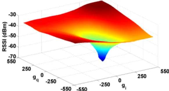
only matches one frequency. This fixed delay suffers from a similar bandwidth constraint as antenna cancellation. Prior work also dis-cusses the limitation of the cancellation model used by QHx220 [9]. The goal of the auto-tuning algorithm in this case would be to find the attenuation factors on both lines such that the QHx220 chip output is the best approximation of the self interference we need to cancel from the received signal. Fortunately, we can show that even with this approximate version, we still retain a psuedo-convex structure. To see this empirically, we conduct an experiment where the TX antenna transmits a 10MHz OFDM signal, and we vary the two attenuations in QHx220. We plot the RSSI output in Figure 8, where a deep null exists at the optimal point. Hence we can use the same gradient descent algorithm for tuning the two attenuation factors in QHx220,giandgq. The algorithm works in steps, and
at each step it computes the slope of the residual RSSI curve by changinggiandgqby a fixed step size. If the new residual RSSI is
lower than before, then it moves to the new settings for the atten-uation factors, and repeats the process. If at any point it finds that the residual RSSI increases, it knows that it is close to the optimal point. It then reverses direction, reduces the step size and attempts to converge to the optimal point. The algorithm also checks for false positives, caused due to noisy minimas. The algorithm is fast; it typically converges to the minimum in8−15iterations, depend-ing on the choice of the startdepend-ing point. An iteration requires 5 mea-surements, each involving a phase/attenuation adjustment followed by RSSI sampling.
Figure 8: RSSI of the residual signal after balun cancellation as we varygiandgqin the QHx220. Note the deep null at the
optimal point.
Caveats: The commodity parts of our prototype introduce a few limitations. The QHx220 has hardware constraints, such that it causes nonlinear distortion, especially for input powers beyond -40dBm. Hence, cancellation will not be perfect for typical wireless input powers (0-30dBm). Non-linear distortion also impacts digital cancellation, as we see in Section 5.1.
Our current implementation uses the QHx220 despite its imper-fections because it is inexpensive and easily available. However, we believe that it is feasible to build a full duplex radio using an electronically tunable delay and attenuation chipset, since they are commercially available but just not widely and inexpensively. Fur-thermore, including them as small parts of a full duplex radio hard-ware design would not be particularly complex or expensive.
3.4
Digital Cancellation
As Figure 5 shows, a industry-grade balun cancellation circuit can cancel up to 45dB of a 40MHz signal. But this cancellation only handles the dominant self-interference component between the receive and transmit antennas. A node’s self-interference may have other multipath components, which, although much weaker than the dominant one, are strong enough to interfere with recep-tion. Furthermore, the balun circuit may distort the cancellation signal slightly, such that it introduces some interference leakage.
The full duplex radio design uses digital cancellation (DC) to cancel any residual interference that persists after balun cancella-tion. Implementing DC for a full duplex radio, however, is more challenging than other uses of digital cancellation, such as succes-sive interference cancellation (SIC) [8] and ZigZag decoding [7]. Unlike SIC or ZigZag, which use DC to recover packets which would have otherwise been lost, a full duplex radio uses DC to pre-vent the loss of packets which a half duplex radio could receive. While an SIC implementation that recovers 80% of otherwise lost packets is a tremendous success, a full duplex radio that drops 20% of packets is barely usable.
To the best of our knowledge, our DC system has three novel achievements compared to existing software radio implementations in the literature. First, it is the first real-time cancellation imple-mentation that runs in hardware: this is necessary for the MAC experiments in Section 5.2. Second, it is the first cancellation im-plementation that can operate on 10MHz signals. Finally, it is the first digital cancellation that operates on OFDM signals. For these reasons, we give a very detailed description of its design and algo-rithms.
Digital cancellation has two components: estimating the self-interference channel; and using the channel estimate on the known transmit signal to generate digital samples to subtract from the re-ceived signal.
Channel Estimation: To estimate the channel, the radio uses known training symbols at the start of a transmitted OFDM packet. It mod-els the combination of the wireless channel and cancellation cir-cuitry effects together as a single self-interference channel, estimat-ing its response. The estimation uses the least square algorithm [15] due to its low complexity. Since the training symbols are defined in the frequency domain – each OFDM subband is narrow enough to have a flat frequency response – the radio estimates the frequency response of the self interference channel as a complex scalar value at each subcarrier. Specifically, letX = (X[0],· · ·, X[N−1])
be the vector of the training symbols used across the N subcarriers for a single OFDM symbol, andMbe the number of such OFDM training symbols. LetY(m),m= 1,· · ·, M, be the corresponding values at the receiver after going through the self interference chan-nel. The least squares algorithm estimates the channel frequency response of each subcarrierk,Hˆs[k], as follows:
ˆ Hs[k] = 1 M " 1 X[k] M X m=1 Y(m)[k] !#
Next, the radio applies the inverse fast Fourier transform (IFFT) to the frequency response to obtain the time domain response of the channel. Upon transmission, it generates digital samples from the time domain response and subtracts them from the observed signal. The time domain response of the self interference channel can be emulated using a standard finite impulse response (FIR) filter in the digital domain. Standard FPGA implementations of the FIR filters are widely available end efficient.
By estimating the frequency response in this way, the least squares algorithm finds the best fit that minimizes overall residual error. The algorithm is more robust to noise in samples than prior ap-proaches, such as simple preamble correlation. Furthermore, un-like more complex algorithms such as minimum mean squared er-ror (MMSE) estimation, which requires a matrix inversion, least squares is simple enough to implement in existing software radio hardware for real-time packet processing.
Applying Digital Cancellation: Next, the radio applies the es-timated time domain channel response to the known transmitted baseband signal and subtracts it from the received digital samples. To generate these digital samples, the hardware convolves the known signal with the FIR filter representing the channel. Lets[n]be the known transmitted digital sample at timenfed into the FIR filter. The outputi[n]of the filter is the linear convolution ofˆhs[n]and
s[n]: i[n] = N−1 X k=0 ˆ hs[k]s[n−k]
After this step, the radio subtracts the estimates of the transmit signal from the received samplesr[n]:
ˆ r[n] =r[n]−i[n] = N−1 X k=0 hd[k]d[n−k] + N−1 X k=0 “ hs[k]−ˆhs[k] ” s[n−k]+z[n],
whered[n]andhd[n]are the transmitted signal and channel
im-pulse response from the intended receiver, andz[n]is additive white Gaussian noise.
3.4.1
Efficacy of Digital Cancellation
Channel estimation accuracy significantly affects digital cancel-lation’s performance. Poor channel estimates can cause the sys-tem to generate digital samples different from what the node hears, such that their subtraction corrupts a received waveform. Accuracy
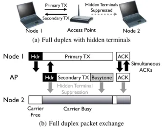
Primary TX Secondary TX Hidden Terminals Suppressed Access Point Node 1 Node 2
(a) Full duplex with hidden terminals
Hdr Node 1 AP Node 2 Primary TX Hdr Secondary TX Busytone Carrier
Free Carrier Busy
ACK ACK Hidden Terminal Suppression Simultaneous ACKs
(b) Full duplex packet exchange
Figure 9: The full duplex MAC protects primary and sec-ondary transmissions from hidden terminal losses. Abusytone
is used to protect periods of single-ended data transfer.
suffers if there is another interfering transmitter present during the channel estimation phase. Hence, the MAC protocol must provide an interference-free period for channel estimation via carrier sense. The second factor is the coherence time of the self interference channel, i.e. the duration over which the channel’s state is sta-ble. A node needs to re-estimate its channel state at a period be-low the channel coherence time. As we explore in Section 5.1, for typical static environment, the channel coherence time of the self-interference channel is on the order of seconds. Hence periodic es-timation at roughly every few hundred milliseconds suffices. How-ever, more frequent or sophisticated techniques may be necessary for highly dynamic mobile environments.
The third and the final factor is possible non-linearities in the self interference channel. Digital cancellation as presented above assumes that the self interference can be modeled as an output of a linear time-invariant system. However, in practice, the balun can-cellation step may introduce a non-linear distortion of the trans-mitted signal which cannot be modeled using an LTI system. As we’ll show in Section 5.1, active components can introduce non-linearities, thus constraining the performance of Digital Cancella-tion.
4.
FULL DUPLEX MAC
The most interesting possible benefits of full duplex occur above the physical layer. Prior work, for example, argued that MAC layer techniques that exploit full duplex can mitigate hidden terminals and improve fairness [4, 13]. However, the lack of a real-time full duplex MAC layer prevented experimentally evaluating these claims. In this section, we describe the design and implementation of a simple full duplex MAC. Later sections evaluate a real-time full duplex network using this MAC. To the best of our knowledge, this is the first implementation of a full duplex MAC that works in real-time on real hardware.
4.1
Design
In CSMA/CA, the hidden terminal problem occurs because a half-duplex receiver cannot inform other nodes of an ongoing re-ception. Full duplexing naturally mitigates the hidden terminal problem because the receiver can immediately start a transmission that also suppresses nearby nodes. Figure 9(a) shows an example.
Node 1 sends a packet to the AP after carrier sense. As soon as the AP receives the header, it starts a transmission back to Node 1. Even if Node 2 is hidden to Node 1, it senses the AP’s transmission and keeps quiet. Thus, in theory, full duplex can prevent hidden terminal collisions.
Furthermore, when a WLAN network is saturated, a bottleneck occurs at the AP because it gets the same transmit opportunity as each client while serving more flows. Full duplexing can remove this bottleneck, since the AP can transmit whenever a client sends a packet to it.
Realizing the benefits of full duplexing requires a full duplex MAC. In a sense, a full duplex PHY creates a parallel channel that a transmitter can simultaneously receive on. However, the parallel channel exists only for transmitters for full duplex: signals add up on other nodes. A full duplex MAC must utilize this rather limited parallel channel in full.
This paper focuses on the simplest case where two full duplexing nodes exchange packets. As suggested by Radunovic et al. [13],a primary transmitterinitiates a transmission via standard CSMA/CA. Once theprimary receiverdecodes the header of the primary trans-mission, it can initiate asecondary transmission.
However, the primary and secondary packets are offset in time and may have different lengths. Therefore, relying solely on data packets does not completely protect from hidden terminals. As Fig-ure 9(b) shows, the AP’s secondary transmission to Node 1 may finish before Node 1’s primary transmission to the AP. Node 2 can transmit and cause a collision when only Node 1 transmits.
Our MAC usesbusytones as a way to mitigate this problem. Whenever a node finishes transmitting a packet before finishing re-ceiving, it transmits a predefined signal until its reception ends. If a node receives a primary transmission and does not have a corre-sponding secondary packet to send, it sends the busytone immedi-ately after decoding the header of the primary packet.
Full duplex mitigates hidden terminals, but does not completely eliminate them. A primary receiver is susceptible to collisions until it has finished receiving the primary transmission’s packet header. In 802.11a, for example, this period is≈56µs, much shorter than a typical data packet.
4.2
Real-Time
The previous section has described the design of a full duplex MAC protocol. Implementing a real-time MAC protocol, however, is not trivial: its low latency contraint imposes certain requirements on the radio hardware. This section focuses on identifying the min-imal features that a full duplex MAC requires, and shows how it is actually implemented.
4.2.1
Challenges
Maximizing the overlap of two transmissions increases through-put and improves collision avoidance. Transmission overlap de-pends on solving two technical challenges, minimizing secondary response latency and having transmission flexibility in preloaded packets.
Secondary response latency: A primary transmission is a “cue” for the secondary transmission to start. A faster response to this cue enables a longer overlap of the two transmissions. The earlier the destination address is in the packet and the faster the hardware can initiate a secondary transmission, the lower the secondary response latency becomes.
Flexibility in preloaded packets: Starting a secondary transmis-sion immediately after primary header reception requires having a packet destined for the primary transmitter already loaded in the
hardware. Having multiple packets loaded increases the probability of having a packet ready for secondary transmission. This calls for the radio driver to have per-destination transmission queues, with the head of each queue preloaded in hardware.
These challenges place requirements on the system hardware. Specifically, the hardware must notify the start of reception once the destination address has been decoded, must be able to start a secondary transmission quickly, and needs enough memory to store multiple transmit packets.
Typical software-defined radios such as USRP [2] cannot meet these requirements, due to latency between hardware and the host PC as well as their need to store packets as digital samples rather than bits. Off-the-shelf WiFi cards also do not meet the require-ments due to the lack of header reception indicators and general difficulty in programming low-level mechanisms such as backoff and clear channel assessments.
4.2.2
Implementation
Our full duplex MAC use the WARP V2 platform [1] from Rice University, which handles physical layer packet processing and latency-sensitive MAC operations in a powerful on-board FPGA. The FPGA can convert packet bits to digital baseband samples on-the-fly, which enables packets to be stored concisely as bits and incorporating dig-ital cancellation. An on-chip embedded processor implements the MAC and auto-tuning algorithm in real-time.
Our MAC implementation is based on the OFDM Reference De-sign v15 [1]. The deDe-sign uses a WiFi-like packet format and 64-subcarrier OFDM physical layer signalling using a 10MHz band-width. Each OFDM symbol is 8µslong, thus QPSK modulation achieves 12Mbps bitrate without any channel coding. The PHY frame has 32µspreamble, followed by 16µstraining sequence, and 24-byte MAC header that is 16µslong.
Primary transmissions use the existing half duplex MAC imple-mentation from the same reference design which mimics 802.11 behavior. For secondary transmissions, the MAC design uses an au-toresponder logic, designed for low-latency link-layer ACK trans-mission. It automatically triggers a secondary transmission if the node detects a primary transmission addressed to it. A measure-ment shows that the latency of this logic is 11µs, which results in the total secondary response latency of 75µsincluding header reception latency.
Each node maintains per-destination transmission queues, and the hardware auto responder logic automatically picks the correct transmission queue to send a secondary packet from based on the header of the primary reception. For primary transmissions, the software maintains a record of the order of arrival of packets from the host computer for different destinations, and sends packets from different queues in the same order.
5.
EVALUATION
This section provides experimental results for the performance of the adaptive full duplex system described in Sections 3 and 4. The evaluation has two parts: physical layer performance of the cancel-lation design and effect of a full duplex MAC on hidden terminals and network fairness.
5.1
Cancellation
We evaluate the cancellation design by measuring how much it can attenuate the self-interference signal. Unlike the cancellation results in Section 3.2, which evaluated the performance of the balun cancellation in isolation, these experiments evaluate the entire radio design.
−30 −25 −20 −15 −10 20 30 40 50 60 70 80 −30 −25 −20 −15 −10 20 30 40 50 60 70 80 Cancellation (dB) Baseline RX Power (dBm) Combined Digital Cancellation Balun Passive Cancellation
Figure 10: Cancellation performance of balun passive cancel-lation combined with digital cancelcancel-lation in a controlled wired setting, where phase and amplitude are controlled by manually tuned, precision passive components. Together they cancel 70-73 dB of self-interference.
5.1.1
Balun Passive Cancellation
In this section we focus on self interference cancellation obtain-able with tunobtain-able passive attenuation and delay components. These components are not electronically programmable: they can only be controlled manually. Consequently we cannot use the passive components when balun cancellation needs frequent tuning, such as wireless channels. We therefore evaluate its performance us-ing a wired setup by connectus-ing the TX and RX antennas usus-ing a wire to simulate a controlled wireless channel. We measure self-interference cancellation obtained with combinations of balun pas-sive cancellation and digital cancellation. As the paspas-sive compo-nents are tuned manually, human imprecision makes it unlikely that the system is at the optimal point: it may be possible to obtain even stronger cancellation with a programmable passive component.
Figure 10 plots the total cancellation obtained for a 10MHz WiFi signal with increasing self-interference power. Passive balun can-cellation, in agreement from the results in Figure 5, cancels around 45 dB of self interference. Digital cancellation can cancel as much as 30 dB: this is 10 dB more cancellation over a sixteen times wider bandwidth, (10 MHz vs 612 kHz), compared to the full duplex ap-proach reported by Duarte et al. [5], which uses two separate TX chains. The 25-30dB of digital cancellation adds on top of the 40-45 dB of balun cancellation to provide a total cancellation of 70-73 dB.
We omit plots for digital cancellation alone for brevity, but report some observations here. Typically, digital cancellation can reduce self-interference by up to 30dB for lower power signals. The per-formance of digital cancellation degrades by up to 9 dB at higher received powers, for example when not using balun cancellation, due to receiver saturation.
The above setup does not benefit from the self interference re-duction from antenna separation between the TX and RX antennas, because they are connected directly by a low loss wire. In prac-tice with wireless channels, we observe around 40dB of attenua-tion (20 cm, 8 inches) from antenna separaattenua-tion with 3dBi antennas. Combined with the 73dB reduction from balun passive cancella-tion, the proposed full duplex design could bring down the self in-terference by up 113 dB. Such cancellation would bring a 20 dBm transmit signal to -93 dBm, close to the noise floor on commodity hardware.
In summary, balun passive cancellation in conjunction with dig-ital cancellation can almost perfectly cancel self interference from wideband signals such as WiFi.
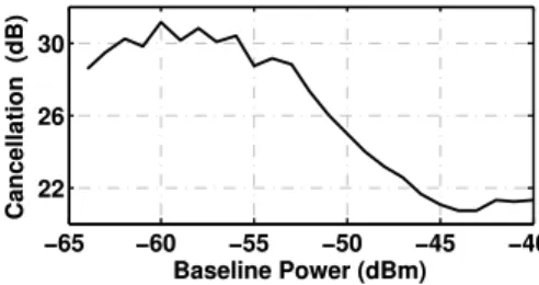
−65 −60 −55 −50 −45 −40 22 26 30 Baseline Power (dBm) Cancellation (dB) −65 −60 −55 −50 −45 −40 22 26 30 Baseline Power (dBm) Cancellation (dB)
Figure 11: Performance of balun active cancellation with in-creasing received power. The QHx220 limits the balun circuit to 30 dB of cancellation at lower powers, and 20 dB at higher powers. Recall from Figure 5 that with passive components the balun circuit can cancel 50 dB over 10MHz.
10 20 30 40 50 60 −0.15 −0.1 −0.05 0 Tap Delay Amplitude 10 20 30 40 50 60 −0.15 −0.1 −0.05 0 Tap Delay Amplitude
(a) Balun passive
10 20 30 40 50 60 −0.1 0 0.1 Tap Delay Amplitude 10 20 30 40 50 60 −0.1 0 0.1 Tap Delay Amplitude (b) Balun active
Figure 12: Real part of the channel estimates for digital cancel-lation with balun passive and balun active cancelcancel-lation. The noise canceler in balun active cancellation introduces non-linearities leading to invalid estimation.
5.1.2
Balun Active Cancellation
As mentioned in Section 3.3.1, active components like QHx220 introduce non-linearities which limit the efficacy of balun and digi-tal cancellation. Figure 11 shows the cancellation achieved with the combination of balun active and digital cancellation as the trans-mit power of the self-interfering signal varies. At an input power of -60 dBm, the circuit can cancel approximately 30 dB. When combined with antenna separation, this cancellation reduces self-interference to the noise floor. As input power increases, how-ever, cancellation deteriorates due to the QHx220’s sub-optimal design. The QHx220 cannot handle a high input power, and be-yond a threshold clips and introduces non-linearities. Furthermore, balun active cancellation reduces the efficacy of digital cancella-tion because QHx220 introduces non-linearities. Since the digital cancellation step is trying to model the self-interference channel as a linear time invariant system, channel estimates are inaccurate and digital cancellation performance suffers.
Figure 12(a) and 12(b) show the issues the non-linearities intro-duce in greater detail. They show the channel impulse response es-timate after the balun cancellation for both passive and active com-ponents. When using passive circuits, the channel estimate con-tains only a few strong taps with small delays. However, with the active QHx220 circuit, the channel estimate has a non-trivial value until the 64th tap, which represents a 1 km long strong multipath component. Such multipath cannot exist: it is an outcome of linear estimation of a non-linear channel.
Our prototype’s dependence on commodity parts such as QHx220 limits its effective performance, limits which an ASIC would not encounter. The results from the previous section suggest that with the availability of electronically programmable attenuation and de-lay components, the above limitations can be remedied.
Convergence Time: While the cancellation the system can ob-tain with QHx220 is limited, we can evaluate how well the
auto-0 10 20 30 40 0 0.2 0.4 0.6 0.8 1 Number of iterations CDF 0 10 20 30 40 0 0.2 0.4 0.6 0.8 1
Figure 13: CDF of Algorithm convergence on hardware. About 30% of the runs have to recover from noisy minimas, but do so quickly. 0 5 10 15 20 25 30 10 15 20 25 30 35 time (seconds) cancellation (dB) 0 5 10 15 20 25 30 10 15 20 25 30 35 Digital Cancellation
Balun Active Cancellation
Figure 14: Performance of balun active cancellation and of dig-ital cancellation over time. Before cancellation, the received power is -45dBm for the balun active cancellation experiment, and -58dBm for digital cancellation. Once tuned, the QHx220 settings are stable for over 10 seconds. The 20 dB maximum is caused by the nonlinearities of the QHx220. Digital cancella-tion performance, on the other hand deteriorates within a span of 3-4 seconds and needs more frequent tuning.
tuning algorithm works in terms of convergence time. Each step in the auto-tuning algorithm measures RSSI for five points along the residual RSSI curve. Each data point takes26µs,10µsto change the QHx220 settings and16µsto measure RSSI over two OFDM symbols. Each iteration therefore takes130µs. Figure 13 shows the cumulative distribution of how many iterations the algorithm takes to converge. The median convergence for the algorithm is8
steps: the average execution time of the algorithm is approximately
1ms. Currently we transmit one short (∼64µs) packet for each RSSI measurement, but the whole process can be fit in one full packet of∼1msduration.
5.1.3
Self-Interference Coherence Time
Figure 14 shows a plot of how auto-tuned balun active cancel-lation and digital cancelcancel-lation decays over time in a daytime of-fice wireless environment. While it takes approximately 1msto tune the balun active circuit, this tuning is typically stable for over 10 seconds. Also, the auto-tuning algorithm can run on-demand: a node should recalibrate when it finds that its noise floor has in-creased when it starts transmitting a beacon or a data packet.
Looking at digital cancellation, immediately after estimation, there is a 32 dB reduction in self interference. Performance quickly degrades over the first two seconds as the channel changes, and af-ter 7 seconds settles at approximately 25 dB. This result makes sense: unlike calibrating balun cancellation, which is mainly for the line-of-sight component between the two antennas, digital can-cellation is handling varying multipath components. A full duplex radio needs to recalibrate its digital cancellation much more fre-quently than its balun cancellation. Each recalibration for digital cancellation takes only a few OFDM symbols.
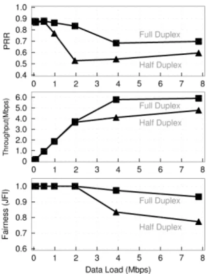
Figure 15: Two upstream UDP flows from two hidden termi-nals to an AP. Full duplexing mitigates collisions due to hidden terminals.
5.2
MAC performance
The previous section proves full duplex feasibility with real-time self interference cancellation over wideband WiFi signals. This section shows that full duplex radios can help solve long standing problems in WiFi MAC. Specifically we focus on the hidden termi-nal and fairness problems.
5.2.1
Hidden Terminals
We setup the following hidden terminal experiment. An AP node is in the middle of 2 nodes which are hidden to each other. Both nodes constantly try to send UDP data to the AP. There is no down-stream traffic from the AP to the nodes. The hidden terminal effect causes packets to collide at the AP, thus causing link layer failures. Since all traffic is unidirectional, full duplex does not increase the capacity in this scenario.
Figure 15 shows the effect of using a full duplex AP in prevent-ing hidden terminals. Both flows maintain a fair throughput until the data load becomes 2Mbps for each flow. At the load of 2Mbps, the Packet Reception Ratio (PRR) for half duplex drops to 52.7%, but full duplex maintains a PRR of 83.4%. Excluding the effect of inherent link losses, full duplex prevents 88% of collision losses because the busy tone of full duplex prevents hidden terminals.
As the data load reaches 4Mbps, the total load exceeds the link capacity. In this case, half duplex cannot maintain both flows due to heavy collisions. The effect can be seen in fairness, which starts to collapse for half duplex. Because there is only one dominant flow active, PRR and throughput for half duplex start to increase.
Full duplex does not perfectly prevent hidden terminal collisions because secondary transmissions start only after header reception. We can see this effect at the data load of 4Mbps, where the PRR of full duplex decreases to 68.3%. Header reception in our PHY reference design takes longer than typical 802.11 PHY, thus we ex-pect the collision avoidance performance of full duplex to be better with 802.11.
5.2.2
Fairness
Table 1 shows experimental results when an AP is connected to four clients. All nodes are within the carrier sense range of each other, thus removing hidden terminal effects. Each node makes
Throughput (Mbps) Fairness
Up Down (JFI)
Half Duplex 5.18 2.36 0.845 Full Duplex 5.97 4.99 0.977
Table 1: Throughput and fairness for four bi-directional UDP flows between an AP and four clients without hidden terminals. Fairness is measured using Jain’s fairness index (JFI). Full du-plexing helps improve the fairness in Wi-Fi like networks.
a bidirectional UDP flow to the AP, making 8 active UDP flows, each with 3Mbps load. The fairness index is computed over the individual throughput of 8 flows.
With half duplex, when traffic is saturated, the AP gets the same share of the channel as all other nodes. However, the AP potentially has four times the traffic as any other node, since it is sending traf-fic to all four nodes. Consequently downstream flows may get an unfairly low share of the channel if the network is fully congested. In our experiment however, we see that the downstream flows do manage to get higher throughput than what we theoretically ex-pect. The reason is that the data load of each flow is 3Mbps, which is lower than the link capacity of around 8Mbps. Consequently, we sometimes have nodes with empty transmit queues that don’t con-tend for the channel, thereby leaving a larger share of the channel for downstream traffic compared to the theoretical throughput limit ofC/(n+ 1), wherendenotes the number of clients andCthe network capacity.
Since the traffic load is bidirectional, it is trivial that full du-plex gets higher throughput than half dudu-plex. However, what is interesting is how full duplex distributes the additional throughput. With full duplex, whenever the AP gets an upstream packet from any node, it is able to send a downstream packet to the same node, thus achieving fairness between upstream and downstream flows. Therefore, full duplex improves the downstream throughput 111%, while the upstream throughput increases only by 15%.
In theory, full duplex should increase the overall throughput by a factor of two, while the results show only a 45% overall increase. The reason is the limited queue sizes at the AP to send to the wire-less clients. Each node can queue 16 packets that come from a host via Ethernet. Due to bursty traffic, sometimes the queue at the AP does not have packets for all clients. If the AP receives a primary transmission from a client and the AP has no packets to respond, the AP loses an opportunity for secondary TX, decreasing through-put. Looking at one of the logs verifies this, where it shows that the AP is able to exploit secondary transmissions for only 52% of the primary receptions.
6.
COMPARISON WITH MIMO
The performance evaluation in the previous section shows the clear benefits of the full duplex in the MAC performance. Can the proposed full duplex also provide any gain over the half duplex in terms of the PHY-layer throughput? In particular, balun cancella-tion requires two antennas and can double the throughput. How-ever, with the same resource, one can build a half duplex multi-input multi-output (MIMO) system which achieves the same gain. This raises a natural question: under what conditions might a wire-less system benefit more from one technique or the other?
If all communication is in one direction, then MIMO performs better, as it doubles the throughput of a single direction. If com-munication is bidirectional, however, the tradeoff is less clear. This section aims to provide some insight on the tradeoffs between half
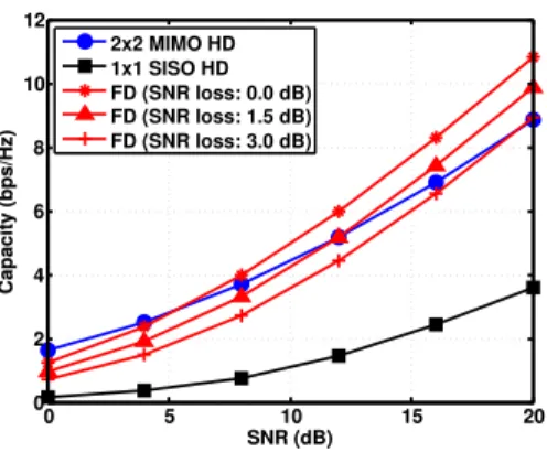
0 5 10 15 20 0 2 4 6 8 10 12 SNR (dB) Capacity (bps/Hz) 2x2 MIMO HD 1x1 SISO HD FD (SNR loss: 0.0 dB) FD (SNR loss: 1.5 dB) FD (SNR loss: 3.0 dB) 0 5 10 15 20 0 2 4 6 8 10 12 SNR (dB) Capacity (bps/Hz)
Figure 16: Capacity comparison of the proposed full duplex system and the2×2MIMO half duplex system
duplex MIMO and full duplex in terms of information theoretic channel capacity under different conditions.
For analyzing the capacity of both a 2x2 MIMO channel and a full duplex channel, we consider the simplest case of 2 nodes trying to constantly send data to each other. Both nodes have 2 antennas that can be used for transmit or receive. We compare the case when the nodes use the two antennas to implement a 2x2 MIMO system vs implement a full duplex system.
We make two assumptions in this comparison namely:
• A wireless node has thesame power constraint during trans-missionregardless of its duplex mode. This means that a half duplex node cannot double its transmit power even though it remains silent half of the time (compared to the full du-plex node which always transmits). This is a more practical condition since FCC regulations and circuit limitations on transmit power restrict the maximum power coming out of a single device regardless of the duplex mode, making it in-feasible to perform such power pulling across time for half duplex nodes. Under this assumption, a 2x2 MIMO system is able to use the maximum power of only a single node at a given time, since only one of two communicating nodes can transmit at a given time. On the other hand, with full duplexing, the system can use the maximum power of both communicating nodes at the same time, thus allowing the use of more total power in system.
• The transmitter knows the state of the wireless channel from itself to the receiver perfectly. For a MIMO system, this increases the capacity by allowing an additional transmitter processing technique, called MIMO precoding. In case of full-duplexing, if both the nodes know the channels between all the antenna pairs, they can agree on the best transmit-receive antenna pair to maximize the sum capacity in both directions. This assumption is valid for most new wireless systems, like 802.11n and LTE, which use periodic feedback to inform the transmitter about the channel state.
Figure 16 shows the 10%-outage capacity of the wireless link for 2x2 MIMO half duplex vs full duplex for different levels of self-interference cancellation performance. The performance of the self-interference cancellation is modeled in terms of the SNR loss due to residual self-interference compared to half duplex. The de-tails of channel capacity analysis for full duplex and 2x2 MIMO half duplex, and the formal definition of the outage capacity are presented in Appendix A.
The figure shows that at low SNR, MIMO half duplex outper-forms full duplex. This result is expected with the diversity gains in MIMO helping its performance for lower SNR values. How-ever, at higher SNRs, full duplex achieves higher average capacity as long as the SNR loss remains below1.5dB. While surprising at a first glance, we can see that such gain actually comes from the power constraint per device allowing full duplex to use twice as much energy use per unit time as compared to MIMO half duplex. Knowing channel state information in practice means different things for a full duplex system and a MIMO system. Channel state information in the full duplex setup allows the system to adaptively pick one of its antennas for transmit, rather than always using the same transmit antenna. This means that a full duplex system only requires a one bit feedback from receiver to transmitter for the full duplex system to exploit some gains of channel state knowledge at the transmitter. MIMO systems, on the other hand, require at least a few bits of feedback to program transmit pre-coders for achieving near-optimal performance [10].
Although not discussed in this section, we have also analyzed the case when the transmitter does not have any information about the state of the wireless channel. Without channel state, the transmitter cannot change its rate in response to channel changes and should fix its rate in advance. In this case, MIMO half duplex outperforms full duplex over the entire SNR range even under ideal cancellation. The spatial diversity of the MIMO system improves the reliability of the wireless channel, thus improving performance for this case. However, having no channel state information may not be a prac-tical scenario for current multi-antenna systems, which always use some form of state feedback for rate adaptation.
This section shows that for different channel conditions the per-formance of full duplex can exceed or lag behind the perper-formance of a similarly resourced 2x2 MIMO system. Interestingly, on top of its superior MAC performance, it is shown that full duplex can also provide better PHY performance at high SNRs.
More importantly, this evaluation shows that MIMO half du-plex and full dudu-plex offer their respective advantages under dif-ferent scenarios: robustness in low SNR scenarios using MIMO, and higher efficiency with full duplex under high SNR. Thus, high performing systems can adopt a hybrid of the two modes depend-ing on the instantaneous channel conditions and the availability of channel state at the transmitter. A significant question going for-ward is whether full duplex can be combined with MIMO systems. If so, this raises an interesting and new degree of freedom.
7.
DISCUSSION
A balun cancellation-based full duplex radio, while an important step forward, leaves several open questions and new possibilities and future research. This section briefly discusses some of them.
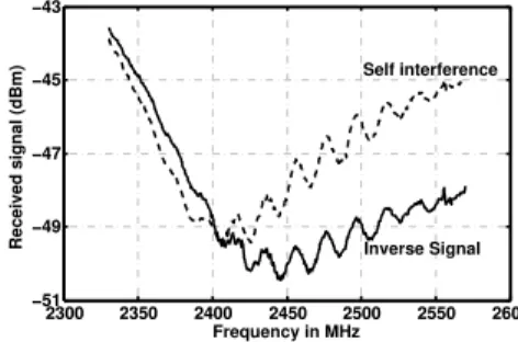
RF Engineering One issue that comes up numerous times in the design is the sensitivity and precision of the components used in cancellation. For example, one early design of the balun cir-cuit had a much less even frequency response, shown in Figure 17. This uneven response was partially from RF echoes in the balun board and placed an upper bound on the maximum cancellation possible. Consider the precision involved: canceling 50 dB of self-interference requires that the inverted signal be within10−5of the reference signal, or 99.999% accurate. These accuracies are clearly possible – a small group of researchers were able to achieve them with commodity components. The practical limitations of balun cancellation remain an open question: if engineered as carefully as mobile phones, for example, much greater cancellation may be pos-sible. The need for in-line high-precision attenuation and delay
cir-2300 2350 2400 2450 2500 2550 2600 −51 −49 −47 −45 −43 Frequency in MHz Received signal (dBm) 2300 2350 2400 2450 2500 2550 2600 −51 −49 −47 −45 −43 Self interference Inverse Signal
Figure 17: Frequency response of a previous version of our balun circuit. The frequency selective mismatch, caused by poor layout, prevented balun cancellation beyond 25 dB.
cuits may introduce additional, practical challenges: the QHx220 is a poor substitute.
Asymmetric Traffic Handling in MACOur current MAC de-sign only sends one secondary packet for a primary packet. How-ever, for asymmetric traffic like TCP, multiple short packets can be transmitted while receiving one long packet. Exploring the effect on the TCP layer may be an interesting future work. More gen-erally, efficiently utilizing the additional capacity of the secondary channel, rather than wasting it with busy tones, is an open question.
In-Packet Channel EstimationThe current full duplex proto-type uses periodic sounding packets for tuning the cancellation mechanisms. This method would suffice for a network with static or slowly moving nodes. For more dynamic environments, the channel state can change very quickly, requiring very frequent es-timation updates. Using in-packet techniques to update channel estimates on a per-packet basis can address this challenge.
Half Duplex CompatibilityOne interesting question going for-ward is how full duplex systems can be incrementally deployed. For example, while the full duplex system presented does not pre-clude coexistence with existing half duplex systems, secondary trans-missions need to know whether the primary is full duplex capa-ble, otherwise there may be poor interactions with link layer retry counts. Or perhaps secondary transmissions should be considered as simple opportunistic receptions.
8.
CONCLUSION
This paper presents design for a full duplex radio based on a novel cancellation technique called balun cancellation. Unlike prior designs, balun cancellation can work on wideband, high power sig-nals, such that it is possible to build full duplex 802.11n devices. These devices can automatically tune their cancellation circuits and so operate in dynamic environments. The paper describes the im-plementation of a full duplex prototype that uses an 802.11-like OFDM link layer which can operate in real time. Using this pro-totype, it evaluates a full duplex MAC layer, validating prior hy-potheses that full duplex can prevent many hidden terminals and improve wireless LAN fairness.
9.
ACKNOWLEDGMENTS
This work was supported by generous gifts from DoCoMo Capi-tal, the National Science Foundation under grants #0832820, #0831163, #0846014 and #0546630, the King Abdullah University of Science and Technology (KAUST), Microsoft Research, scholarships from the Samsung Scholarship Foundation, a Stanford Graduate Fellow-ship and a Stanford Terman FellowFellow-ship. We would like to thank Mango Communications, especially Patrick Murphy, for timely