Munich Personal RePEc Archive
On The Use and Misuse of Input-Output
Based Impact Analysis in Evaluation
Grady, Patrick and Muller, R. Andrew
Global Economics Ltd., Department of Economics, McMaster
University
12 May 1986
Online at
https://mpra.ub.uni-muenchen.de/22063/
ON THE USE AND MISUSE
OF INPUT-OUTPUT
BASED
IMPACT
ANALYSIS
IN EVALUATION
edcbaZYXWVUTSRQPONMLKJIHGFEDCBAb y
Patrick
Grady
and
R.
Andrew
Muller
Table of Contents
1 INTRODUCTION
2 EXAMPLES
OF THE MISUSE
OF IMPACT ANALYSIS
1
6 CONCLUSIONS
edcbaZYXWVUTSRQPONMLKJIHGFEDCBA3 5 9
13
2 0
3 INPUT-OUTPUT
MODELS
4 MULTIPLIERS
FROM MACROECONOMIC
MODELS
1 INTRODUCTION
Estimates of the output and employment impacts are often
an important part of many program and project evaluations.
The analytical framework frequently used to prepare these
estimates is the family of input-output models developed and
maintained by Statistics Canada. The output and employment
multipliers derived from input-output models are used to
translate the direct impact of a program into its total
impact. The total impact estimated using the "closed"
version of the input-output .model includes the output and
employment generated by subsequent rounds of spending of the
income created by the initial program expenditure. It thus
reflects the traditional Keynesian multiplier taught in all
"
.
the introductory economic textbooks.
Frequently, the output and employment impacts of a program
are treated as though they were "benefits" of the program or
project. They may be explicitly tabulated as benefits.
Alternatively they may be implicitly treated as such by
bearing labels like "jobs created" or by being compared to
In this paper, we argue that such estimated output and
employment impacts in program or project evaluation are
often used inappropriately. There are two reasons why this
occurs. First, many evaluators are not aware that the
multipliers they use make very strong and often untenable
assumptions about macroeconomic impacts. The best evidence
that is currently available suggests that multipliers
.derived from input-output models overestimate the impact of
.changes in government expenditures by ignoring the critical
macroeconomic feed backs that tend to reduce the multiplier
over time. This dramatizes the need to separate the
analyses of the microeconomic and macroeconomic impacts of
programs and projects. Second, many evaluators have an
inadequate understanding of the principles of cost-benefit
analysis. They thus tend to confuse the output and
employment impacts of a program with its benefits. This is
a tendency that has been exacerbated by the emphasis in the
current guidebooks on program evaluation on procedure to the
virtual exclusion of any discussion of the principles of
cost-benefit analysis.[l]
Section 2 of the paper offers two examples of the misuse
of output and employment impacts estimated using
input-output techniques. Section 3 the paper briefly
discusses some of their limitations. It also presents
estimates of the multipliers derived from them. Section 4
provides the details of our criticism of the use of
input-output multipliers from a macroeconomic point of
view. The main macroeconomic feedbacks that tend to dampen
the reponse of the economy to government spending shocks are
outlined and estimates of multipliers from the main Canadian
macroeconomic models are presented. Section 5 reviews the
connection between economic impact analysis and cost-benefit
analysis. It emphasises a number of reasons why employment
impacts cannot uncritically be considered benefits of a
program or a project. Section 6 gives our conclusions.
2 EXAMPLES OF THE MISUSE OF IMPACT ANALYSIS
As recent examples of the pervasive misuse of economic
impact analysis we consider a provincial position paper on
housing policy and a published evaluation of benefits from
irrigation expenditures in Alberta. These two provincial
examples were chosen because they have been published.
Federal examples can be found in some of the unpublished
departments. Most readers will thus
phenomenon from their own experience.
recognize the
In a position paper issued last December, the Ontario
government a number of initiatives to stimulate the
construction of new housing.[2] These included interest-free
loans to private rental developers, changes to the rent
review system, increased social housing and a strategy to
,stimulate the building industry. A table in the doc~ment
"provides an overall picture of the estimated impact of the
programs". In aggregate a provincial expenditure of $480
million was expected to induce $5.2 billion of construction
expenditures and to "create" almost 200,000 job-years of
employment. Footnotes indicated that a multiplier of 2.2
person years was used throughout the calculation. The table
leaves the clear impression that the programs can create
emploiment at a cost to the government of $2410 per
job-year.
o
As a·second example, Kulshreshtha et.al.[3] report ona
study conducted for the Alberta Irrigation Projects
Association. Here the goal was explicitly to identify the
major beneficiaries of irrigation activity. Input-output
calculations showed that capital expenditures of about $348
benefits" of $415 million per year. Only 15 per cent of
these benefits would be received by water users. The
remainder would be distributed throughout the economies of
Alberta and the rest of Canada. Taken at face value, these
results imply an annual return on investment of about 119
per cent!
What is wrong with these analyses? Our contention is that
they, and many like them, confuse economic impacts .with
economic benefits. Even when this confusion is resolved,
they exaggerate
comparing them
the impacts of programs and
to the wrong benchmark
projects by
and by using
excessively high multipliers to compute induced effects. 'In
the next two sections we review how the multipliers are
derived and how they compare to those estimated from large
macroeconomic models. We then return to the relationship
between benefits and impacts.
3 INPUT-OUTPUT MODELS
Input-output models are designed
changes in final demand such as consumer
the impact of
expenditures,
investment and government spending on the structure of
output and employment by industry, sector or province.
Statistics Canada has developed a whole family of
input-output models for Canada which can be used for various
types of impact analysis.[4] These include inter-provincial,
price and energy models as well as the basic output
determination model.
An input-output model can be used to estimate the impact
on output and employment by industry of government
expenditures on particular programs or projects. For
example, the impact on the economy of a construction project
such as building a road could be estimated. The
input-output model would show the direct impact of the
initial spending on the project on the final demand category
government expenditures on non-residential construction.
The i~~ut-output model would then transform this spending
into spending on intermediate material inputs such as
concrete, steel rods, gravel and fuel and into spending on
the primary inputs of labour, capital and indirect taxes.
Spending on inputs would in turn be transformed into
industry outputs producing estimates of the indirect impact
of the initial increase in spending. Employment/output
coefficients are used to transform industry output impacts
estimate of the total (direct plus indirect) impact of the
initial increase in spending on output and employment by
industry. If the inter-provincial model were used, a
regional dimension could be added to the estimates of output
and employment by industry.
There are two versions of the output determination model.
One is the "open" model in which all final demand categories
including consumption are treated as exogenous. In this
model the income generated in the process of production is
not assumed to be respent. The second version is the.
"closed" model in which the income generated by the
production process that accrues to the household sector is
assumed to be either spent on goods and services or taxes or
to be saved in accordance with average past proportions.
These effects are called "induced." The "closed" model
exhib~ts a traditiona1 textbook Keynesian multiplier when
subjected to exogenous expenditure shocks. The magnitude of
the multiplier varies inversely with the magnitude of the
leakages from the expenditure stream for non-wage income,
taxes, savings, and imports.
The impact multipliers derived from the "open" and
"closed" versions of the output determination model are
a $1 million exogenous increase in spending on residential
construction, the "closed" model yields a multiplier of 1.66
(the ratio of the the impact on
GDP
at market prices to theinitial expenditure increase), whereas the "open" version of
the model only yields a multiplier of .89 (the difference
from unity reflecting import leakages).
There are some features of input-output models of which
those concerned with evaluation should be aware. First,
input-output models are static. There is no time dimension
attached to their impact estimates, which represent
equilibrium results. Second, the models are linear. This
entails an assumption of proportionality between inputs and
outputs, between total income and its components, and
between employment and output. Such an assumption can be
particularly inapppropriate in making estimates of short run
emplofment multipliers. As a rule, employment responds much
less than one-far-one with output increases due to the
overhead character of some labour and to the occasional
prevalence of a certain degree of labour hording. Third,
input-output models do not incorporate macroeconomic
feedbacks which tend to reduce the impact multipliers. This
4 MULTIPLIERS
FROM
MACROECONOMIC
MODELS
The multiplier results derived from a closed input-output
system yield exaggerated estimates of the impact of program
expenditures on the economy. This is the case because
closed input-output models do not take into account the
macroeconomic feedbacks that tend to cause the multiplier to
decrease over time. The principal feedbacks for 'government
spending programs are the same as for any other type of'
expenditures. Higher spending raises demand and hence
~utput and employment. Increased capacity utilization and
reduced unemployment puts upward pressure on prices and
wages. Greater real output and a higher price level results
in increased nominal income. This in turn causes interest
rates to go up provided that money growth is fixed. Higher
interest rates and prices serve to erode the initial demand
stimulus, thus decreasing the multiplier.
The feedback effect of interest rates and the financial
sector depend very much on the financing assumption made.
The usual assumption is that the increase in government
spending is debt financed. Monetary policy can be assumed
'.mlkjihgfedcbaZYXWVUTSRQPONMLKJIHGFEDCBA
that the money supply growth is either assumed to be
unchanged or allowed to increase in response to the
increased spending. If it is non-accomodating, debt
financed increases in government expenditure will have a
larger effect on interest rates. Alternatives to the debt
financing assumption are that expenditure increases are
financed by tax increases or reductions in other government
spending. The implications of such alternative assumptions
are vastly different. The only way to take them into
account is at the level of overall fiscal policy
fomu1ation. This can not be done at the level of the
individual program or project.
A better appreciation of how these macroeconomic factors
tend to decrease the value of the multiplier in the
longer-run can be gained by considering the results of
simu1ations with' macroeconomic models. Table 1 presents the
results of a $1 billion government expenditure shock for the
main Canadian macroeconomic models that participated in a
Bank of Canada - Department of Finance sponsored seminar
held in Ottawa in July, 1982.[5] The models included are:
QFS - the Quarterly Forecasting and Simulation Model of the
Department of Finance; RDXF the Research Department
Experimental Forecasting Model of the Bank of Canada; the
of the Canadian Economy of Data Resources Canada; FOCUS
the Forecasting and User Simulation Model of the Institute
for Policy Analysis, University of Toronto; TIM - the
Informetrica Model of Informetrica Ltd.; CANDIDE 2.0 of the
Economic Council of Canada; SAM - the Small Annual Model of
the Research Department of the Bank of Canada; and MACE
-the Macroeconomic and Energy Model of Professor John
Helliwell of the University of British Columbia.
The noteworthy feature of these results is the extent to
which the multiplier declines over time for almost all the
models - the DRI model being the only exception. On
average, by the fifth year, the multiplier was less than one
and by the tent~ year it was not very much greater than
zero. Some of the models such as FOCUS, SAM and MACE even
had negative multipliers. This suggests that in the medium
term ~he indirect effects of government spending are
negative and growing.
The conclusions to be drawn are that there is much
uncertainty about the medium-to-long-run value of
multipliers and that any estimate of the impact of
government spending programs based on input-output
multipliers which ignore macroeconomic feedbacks are likely
rmlkjihgfedcbaZYXWVUTSRQPONMLKJIHGFEDCBA
government spending programs are more likely to be negative
than positive.
While not perhaps as much as might be expected, the model
estimates of the multiplier depend on the degree of capacity
utilization assumed for the economy. Consequently, it is
necessary to consider the overall economic situation and
total government expenditures and revenues in order to
accurately gauge the impact of government spending on the
economy. There is also the issue of the financing of the
expenditure increase that can only be taken into account in.
the context of the overall formulation of fiscal policy.
Given the great uncertainty concerning the indirect effect
of government spending programs and the importance of
determining the setting of fiscal policy centrally, the most
prudent course for those responsible for evaluating programs
and projects would be to confine their estimates of the
output and employment impacts to the direct impacts and to
leave ·the question of the indirect impact to those
5 ECONOMIC IMPACTS AND COST BENEFIT ANALYSIS
In this section we comment on the relationship between
cost-benefit analysis and economic impact analysis and
restate some long known but insufficiently heeded objections
to the exaggeration of the employment and output gains
through the use of multipliers and to the uncritical
treatment of impacts as benefits. We do not attempt to
replicate the excellent introductions to the theory and
practice of cost-benefit analysis which can be found, for
example, in the Treasury Board's Benefit-Cost Analysis
Guide.[6]
The economic impact of a progam or activity is the change
it induces in an economic indicator, such as GNP or
employment. To calculate a change, one must compare the
results of the program or project to what might reasonably
be expected to occur in its absence. This is the benchmark
or basis of comparison. In many evaluations, these impacts
are implicitly or explicitly treated as "benefits" of the
housing policies in the study mentioned above were reported
under the heading "Jobs Created" and the Kulshreshtha study
used the terms "impact" and "benefit" interchangeably.
One difference between cost-benefit analysis and economic
impact analysis is that cost-benefit analysis places a much
stricter interpretation on the term "benefit". The benefit
of the program or project is the gain realized by
undertaking it. In cost-benefit analysis. benefits. are
measured by what people are willing to pay for them.
Similarly the negative impacts (costs) of a program o~
project are valued at what people are prepared to pay to
avoid them. These definitions are consistent with the
common sense proposition that a project is worth undertaking
only if its benefits exceed its costs.
A second difference lies in the choice of benchmarks.
Like economic impact analysis, cost-benefit analysis employsedcbaZYXWVUTSRQPONMLKJIHGFEDCBA
a benchmark for purposes of comparison. When using
input-output analysis to assess impacts, the usual benchmark
is a world in which the program or project does not exist
and nothing takes its place. It is implicitly assumed that
all the labour, capital and other resources used in
activities affected by the program would have otherwise been
consider the alternative uses of the resources in question.
Normally it is assumed that they could have found other
employment at the same wage, but techniques exist to adjust
for the presence of unemployment in special cases. The
correct treatment of employment gains is considered in the
literature on the social opportunity cost of labour.[7]
Briefly, the net gain from the creation of a permanent job
is estimated to range from zero to 25 per cent of the wage
bill (depending on the rate of growth of the region), while
the creation of temporary jobs may actually impose a cost of
up to 30 to 50 per cent of the wage bill by increasing the
pool of workers who experience regular bouts of temporary
unemployment.
To illustrate these points, consider the impact of the
Ontario housing policies. The estimate that 200,000 jobs
would i be created cwas made by multiplying by 2.2 the
estimated number of housing starts associated with each
policy. The multiplier of 2.2 jobs per housing start can be
derived from input-output models by adding up all direct,
indirect and induced effects. The benchmark being used,
therefore, is an economy in which none of the housing starts
occur and no other activity takes their place. But from the
viewpoint of cost-bene~it analysis, this is an unacceptable
the program other activities would have occurred. For
example, the $480 million might have been spent on highway
construction or returned to taxpayers by cutting taxes.
Either alternative would create jobs and income and either
alternative would have induced effects that could be
estimated using a multiplier. The true impact of the
housing program is the difference between the jobs and
income created under it and those created under a reasonable
alternative. (These "differential" impacts may be positive
or negative). The benefits of the program, properly
speaking, should be measured by how much we are willing to
pay to achieve these differential impacts. Similarly, the
Kulshreshtha study calculates the impact of continued
irrigation by computing the direct, indirect and induced
impact of the construction expenditures and the associated
increase in crops. All of the increase in
GDP
is counted a benefit of the project. But a better benchmark would be thepattern of economic activity in Alberta and Canada if the
resources used by the irrigation project were used elsewhere
in the economy to generate higher outputs in other
industries. The value of the output foregone elsewhere can
be approximated by the payments formerly made to the labour
and other resources now used in irrigation. The benefits of
increased earnings of land, labour and capital employed in
irrigation rather than in their best alternative uses.
These examples illustrate why the employment changes
estimated using input-output analysis or multipliers should
never be treated as benefits. More formally, employment
changes ("impacts") cannot be tieated as benefits for at
least three reasons.
First, the employment created by a project or program will
almost never increase net employment in the region by a
corresponding amount, since the employees attracted to the
project need not be replaced. Even less will the project
reduce unemployment, becauEe the increased demand for labour
will cause the labour force to grow through migration and
new entry. The creation of temporary jobs may even increase
the pool of workers experien~ing temporary unemployment.
Second, it is both difficult and unwise to use impact
analysis to calculate the net increase in employment
attributable to a program. To do so requires an explicit
judgement on how public funds would be expended in its
absence and how macroeconomic feed backs would affect the
final outcome. Even in the best of circumstances, this
requires the knowledge and expertise of specialists' in
government, like most western governments, has been
organized to reflect three goals of government expenditure
and taxation: stabilization, allocative efficiency and
income redistribution. [8] The Department of Finance and
the Bank of Canada are responsible for advising the
government on stabilization policy, including attempts to
influence the level of output and employment and the rate of
inflation. The Treasury Board and the program departments
are responsible for advice on resource allocation and
program delivery. Given this division of labour, it is
inappropriate for program departments to evaluate their
programs and projects from the point of view of
stabilization policy. This is best left to the Department
of Finance, where the expertise and information required to
carry out the task is concentratedc
Finally, it is not always true that increased employment
is an unambiguous good. This point is often expressed by
saying that the unemployed and those not in the labour force
value their leisure. By leisure is meant much more than
idle time. For example, consider a policy which enables
mothers to enter the labour force by providing subsidized
day care. The mother incurs a cost both in lost time
available for housework and shopping as well as for
caring for her children. This cost, together with the total
cost of day care subsidy, may easily outweigh her ea~nings.
Under these circumstances everyone would be better off if
she were provided an income transfer sufficent to allow her
to stay at home. In this case, increased employment is not
synonymous with increased welfare.
If impact analysis cannot be used to estimate the benefits
of a program, what can it be used for? An appropriate,role
is to identify regions and industries that will be
particularly affected by a project or program. Input-output
analysis is well suited to this purpose. Note, however,
that it is the open model which is appropriate in this
case. The induced effects measured by the closed model will
be similar regardless of the program analysed. And even
when the open model is used the analyst must be careful to
note ~hat the impacts are not net o,f offsetting changes
induced by foregoing alternative programs. For that reason
it should be unacceptable to use employment impacts to
measure "job creation".
The preceding discussion indicates that economic impact
analysis has many similarities with cost-benefit analysis.
The difference is that cost-benefit analysis attempts to
of a systematic evaluation of the benefits and costs of
alternative actions. While many reservations have been
expressed about the details of cost-benefit analysis and the
practicality of reducing all costs and benefits to a common
scale of dollars and cents, this should not excuse other
analysts from committing fallacies which basic cost-benefit
analysis helps to avoid.
6 CONCLUSIONS
Estimates of the output and employment impacts' of
government programs and projects prepared using the closed
input-output model should not be used in evaluations. It is
more i~portant that the evaluators concentrate their efforts
on producing the most reliable direct impact estimates and
in applying the microeconomic allocative tool of
cost-benefit analysis. The measurement of the indirect
(macroeconomic) impacts of government spending can with a
few exceptions be best carried out at a higher level of
aggregation and can be best left to those specializing in
This is not to suggest that the input-output model should
be banned entirely from the evaluator's toolbox. There will
still be many instances in which it will be an appropriate.
These include the use of the open input-output model to
provide estimates of the industrial or regional breakdown of
the direct impact of a program or of the employment impacts
of program spending. For these particular uses, estimates
derived from the input-output model may be either the most
reliable or most cost-effective estimates it is possible to
FOOTNOTES
1. Treasury Board of Canada, Comptroller General,Principles for the Evaluation of Programs by Federal Departments and Agencies, (Ottawa: Supply and Services Canada, 1981) and Guide on the Program Evaluation Function, (Ottawa: Supply and Services Canada, 1981).
2. Government of Ontario, Ministry of Housing, Assured Housing for Ontario: A Position Paper, December 1985.
3. Surendra N. Kulshreshtha, K. Dale Russell, Gordon Ayers, and Byron C. Palmer, "Economic Impacts of Irrigation Development in Alberta Upon the Provincial and Canadian Economy," Canadian Water Resources Journal, vol. 10, no.2
(1985), pp.l-l0.
4. See Statistics Canada, Users' Guide to Statistics Models, February 1986.
Structural Canada's Analysis Structural Division, Economic
5. Brian O'Reilly, Graydon Paul in and Philip Smith, "Responses of Various Econometric Models to Selected Policy Shocks," Technical Report 38, Bank of Canada, July 1983.
6. Tr~asury Board of Canada, Benefit Cost Analysis Guide (Ottawa: Department of Supply and Services, 1976).
7. See Employment and Immigration Canada, Task Force on Labour Market Development, Labour Market Developments in the 1980s,' July 1981, Appendix A, pp. 211-219 and A.C. Harberger, "The Social Opportunity Cost of Labour: Problems of Concept and Measurement as Seen from a Canadian Perspective," a paper prepared for the Task Force on Labour Market Development.
· .1 ~
T A B L E 1
T H E IM P A C TO F A $ 1 B IL L IC N IN C R E A S EIN F E D E R A LC lJR R F N I'N a l-W A G E E X P E N D I'IU R E SE S T L '1 A T E DU S IN G C A N A D IA NM A C R O -~ IC M O O E L S (D iffe re n c e b e tw e e n sh o c k e d a n d c o n tro l sim u la tio n s)
tn )E L
••
Q F S R D X FC H A S E( 1 ) OR! F C X :U S T IM (2 ) C A N D ID E2 .0 S A M M A C EA V G .(3 )
R E A L G N E(% )
Y E A R 1 0 .3 2 0 .2 8 0 .8 0 .3 3 0 .2 2 0 .4 6 0 .5 5 0 .0 9 0 .1 8 0 .2 8 Y E A R 3 0 .3 8 0 .1 4 0 .4 0 .2 7 0 .2 4 0 .4 3 0 .6 0 0 .0 7 0 .0 5 0 .2 5 Y E A R5 0 .3 1 0 .0 7 0 .2 0 .2 6 0 .0 1 0 .3 6 0 .4 6 0 .0 6 0 .0 0 0 .1 7 Y E A R1 0 0 .1 4 0 .0 1 0 .0 0 .2 4 -0 .0 6 0 .2 8 0 .1 7 -0 .1 0 -0 .1 8 0 .0 3 E M P L O Y M E N l'(')
Y E A R1 0 .1 8 n a 0 .6 0 .1 6 0 .1 5 0 .1 9 0 .2 8 0 .0 0 0 .0 6 0 .1 4
N
Y E A R 3 0 .5 5 n a 0 .4 0 .2 3 0 .3 5 0 .3 4 0 .4 2 0 .0 3 0 .0 9 0 .2 8
tN
Y E A R5 0 .2 9 n a 0 .1 0 .1 8 0 .0 0 0 .4 0 0 .3 7 0 .0 4 0 .0 9 0 .1 6 Y E A R1 0 -0 .0 3 n a -0 .4 0 .1 7 0 .1 2 0 .2 8 0 .2 5 0 .0 2 0 .0 7 0 .1 0 R E A L M U L T IP L IE R
Y E A R1 1 .0 4 1 .0 9 1 .1 1 .4 4 1 .0 5 1 .6 7 1 .9 8 0 .4 2 0 .7 5 1 .1 1 Y E A R 3 1 .3 1 0 .5 8 0 .5 1 .2 3 1 .2 4 1 .7 2 2 .2 5 0 .1 4 0 .2 2 1 .0 0 Y E A R5 1 .1 1 0 .3 4 0 .2 1 .2 5 0 .0 7 1 .5 2 1 .8 5 -0 .2 7 0 .0 0 0 .6 2 Y E A R1 0 0 .6 4 0 .0 6 0 .0 1 .4 8 -0 .4 4 1 .4 1 0 .7 7 -0 .2 3 -1 .0 0 0 .1 8
(1 ) T o ta l fe d e ra l g o v e rn ro o n t e x p e n d itu re s. (2 ) N a n in a l in te re st ra te fix e d .
[image:26.796.7.789.15.596.2]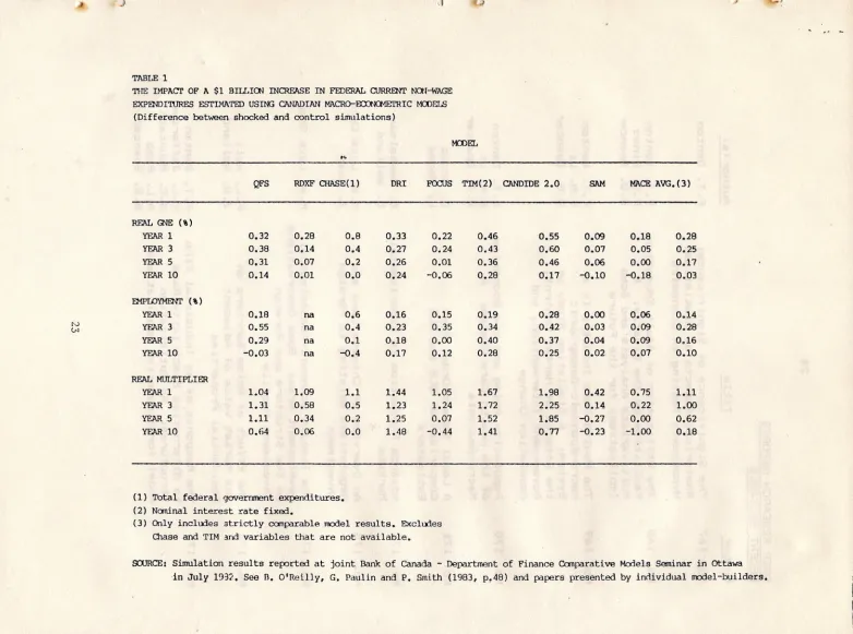
 XXX draft](data:image/gif;base64,R0lGODlhAQABAIAAAP///wAAACH5BAEAAAAALAAAAAABAAEAAAICRAEAOw==)