Hyperparameter Optimization Of Deep Convolutional Neural Networks Architectures For Object Recognition

(1)

HYPERPARAMETER OPTIMIZATION OF DEEP

CONVOLUTIONAL NEURAL NETWORKS

ARCHITECTURES FOR OBJECT RECOGNITION

Saleh Albelwi

Under the Supervision of Dr. Ausif Mahmood

DISSERTATION

SUBMITTED IN PARTIAL FULFILMENT OF THE REQUIREMENTS FOR THE DEGREE OF DOCTOR OF PHILOSOPHY IN COMPUTER SCIENCE

AND ENGINEERING THE SCHOOL OF ENGINEERING

UNIVERSITY OF BRIDGEPORT CONNECTICUT

(2)

(3)

iii

HYPERPARAMETER OPTIMIZATION OF DEEP

CONVOLUTIONAL NEURAL NETWORKS

ARCHITECTURES FOR OBJECT RECOGNITION

(4)

iv

ABSTRACT

Recent advances in Convolutional Neural Networks (CNNs) have obtained promising results in difficult deep learning tasks. However, the success of a CNN depends on finding an architecture to fit a given problem. A hand-crafted architecture is a challenging, time-consuming process that requires expert knowledge and effort, due to a large number of architectural design choices. In this dissertation, we present an efficient framework that automatically designs a high-performing CNN architecture for a given problem. In this framework, we introduce a new optimization objective function that combines the error rate and the information learnt by a set of feature maps using deconvolutional networks (deconvnet). The new objective function allows the hyperparameters of the CNN architecture to be optimized in a way that enhances the performance by guiding the CNN through better visualization of learnt features via deconvnet. The actual optimization of the objective function is carried out via the Nelder-Mead Method (NMM). Further, our new objective function results in much faster convergence towards a better architecture. The proposed framework has the ability to explore a CNN architecture’s numerous design choices in an efficient way and also allows effective, distributed execution and synchronization via web services. Empirically, we demonstrate that the CNN architecture designed with our approach outperforms several existing approaches in terms of its error rate. Our results are also competitive with art results on the MNIST dataset and perform reasonably against the state-of-the-art results on CIFAR-10 and CIFAR-100 datasets. Our approach has a significant role in

(5)

v

increasing the depth, reducing the size of strides, and constraining some convolutional layers not followed by pooling layers in order to find a CNN architecture that produces a high recognition performance.

Moreover, we evaluate the effectiveness of reducing the size of the training set on CNNs using a variety of instance selection methods to speed up the training time. We then study how these methods impact classification accuracy. Many instance selection methods require a long run-time to obtain a subset of the representative dataset, especially if the training set is large and has a high dimensionality. One example of these algorithms is Random Mutation Hill Climbing (RMHC). We improve RMHC so that it performs faster than the original algorithm with the same accuracy.

(6)

vi

ACKNOWLEDGEMENTS

My thanks are wholly devoted to God, who has helped me complete this work successfully. I owe a debt of gratitude to my family for their understanding and encouragement. I am very grateful to my father for raising me and encouraging me to achieve my goal. Special thanks go to my wife and my kids; I could have never achieved this without their support.

I would like to express special thanks to my supervisor Dr. Ausif Mahmood for his constant guidance, comments, and valuable time. Without his support, I would not have been able to finish this work. My appreciation also goes to Dr. Khaled Elleithy for his feedback and support, and to my committee members Dr. Miad Faezipour, Dr. Prabir Patra, Dr. Xingguo Xiong, and Dr. Saeid Moslehpour for their valuable time and suggestions.

(7)

vii

LIST OF TABLES

Table 4.1 Hyperparameter initialization ranges 58

Table 4.2 Error rate comparisons between the top CNN architectures obtained by our objective function and the error rate objective function via NMM

59

Table 4.3 Error rate comparison for different methods of designing CNN architectures on CIFAR-10 and CIFAR-100. These results are achieved without data augmentation

60

Table 4.4 Comparison of execution time by serial NMM and parallel NMM for Architecture Optimization

63

Table 4.5 Error rate comparisons with state-of-the-art methods and recent works on architecture design search. We report results for CIFAR-10 and CIFAR-100 after applying data augmentation and results for MNIST without any data augmentation

64

Table 4.6 Uniform CNN architecture summary 68

Table 4.7 Illustrates the accuracy of different instance 68 Table 4.8 Running time comparison between original RMHC and

our proposed approach of RMHC for one iteration

69

(11)

xi

databases, including individual classifiers and MC systems

Table 4.10 Performance of classifiers with the replacement of classifiers with SA in the last stage

(12)

xii

LIST OF FIGURES

Figure 2.1 The standard structure of a CNN 10

Figure 2.2 Sparse Autoencoder structure: The number of units in input layer is equal to number of units in output layer

24

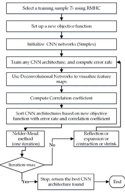
Figure 3.1 General components and a flowchart of our framework for discovering a high-performing CNN architecture

33

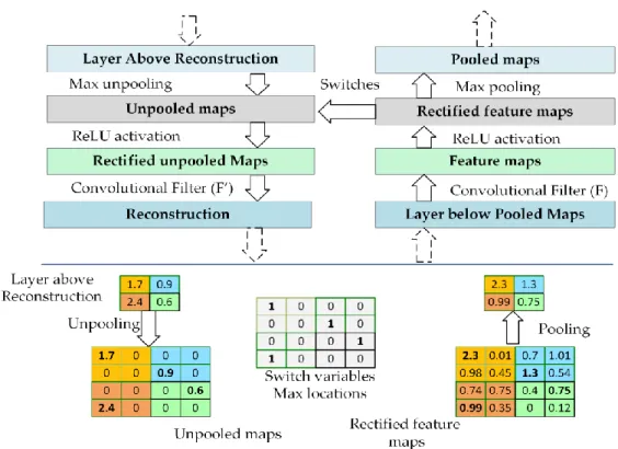
Figure 3.2 The top part illustrates the deconvnet layer on the left, attached to the convolutional layer on the right. The bottom part illustrates the pooling and unpooling operations [14]

36

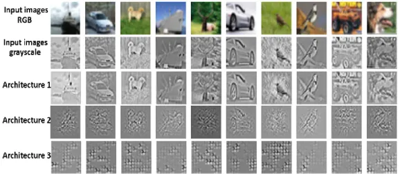
Figure 3.3 Visualization from the last convolutional layer for three different CNN architectures. Grayscale input images are visualized after preprocessing

37

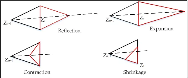
Figure 3.4 Nelder Mead method operations: reflection, expansion, contraction, and shrinkage

42

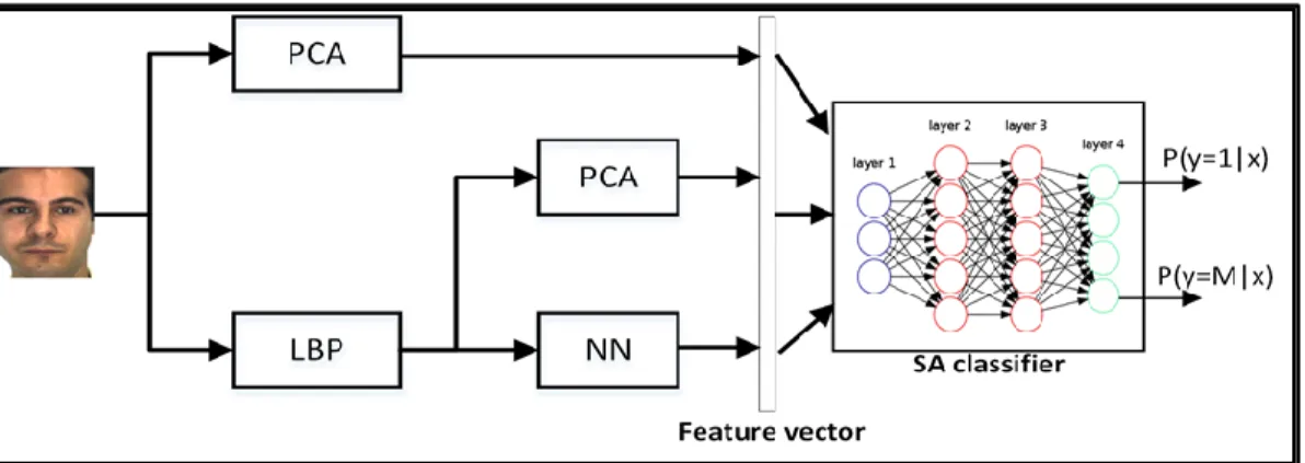
Figure 3.5 Our proposed system for face recognition 49 Figure 3.6 LBP operator computation for a 3×3 grid [103] 51 Figure 3.7 An architecture of stacked sparse autoencoder (SSA) that

consists of two hidden layers

52

(13)

xiii one class

Figure 4.2 Objective functions progress during the iterations of NMM. (a) CIFAR-10; (b) CIFAR-100

61

Figure 4.3 The average of the best CNN architectures obtained by both objective functions. (a) The architecture averages for our framework; (b) The architecture averages for the error rate objective function

62

Figure 4.4 The running speed with different values of k. 70 Figure 4.5 Performance of all proposed classifiers in Tables 4.9 and

Table 4.10.

(14)

1

CHAPTER 1: INTRODUCTION

Deep convolutional neural networks (CNNs) recently have shown remarkable success in a variety of areas such as computer vision [1-3] and natural language processing [4-6]. CNNs are biologically inspired by the structure of mammals’ visual cortexes as presented in Hubel and Wiesel’s model [7]. In 1998, LeCun et al. followed this idea and adapted it to computer vision. CNNs are typically comprised of different types of layers, including convolutional, pooling, and fully-connected layers. By stacking many of these layers, CNNs can automatically learn feature representation that is highly discriminative without requiring hand-crafted features [8, 9]. In 2012, Krizhevsky et al. [1] proposed AlexNet, a deep CNN architecture consisting of seven hidden layers with millions of parameters, which achieved state-of-the-art performance on the ImageNet dataset [10] with an error test of 15.3%, as compared to 26.2% obtained by second place. AlexNet’s impressive result increased the popularity of CNNs within the computer vision community. Other motivators that renewed interest in CNNs include the number of large datasets, fast computation with Graphics Processing Units (GPUs), and powerful regularization techniques such as Dropout [11]. The success of CNNs has motivated many to apply them to solving other problems, such as extreme climate events detection [12] and skin cancer classification [13], etc.

(15)

2

Some works have tried to tune the AlexNet architecture design to achieve better accuracy. For example, in [14], state-of-the-art results are obtained in 2013 by making the filter size and stride in the first convolutional layer smaller. Then, [3] significantly improved accuracy by designing a very deep CNN architecture with 16 layers. The authors pointed out that increasing the depth of the CNN architecture is critical for achieving better accuracy. However, in [15, 16] showed that increasing the depth harmed the performance, as further proven by the experiments in [17]. Additionally, a deeper network makes the network more difficult to optimize and more prone to overfitting [18].

The performance of a deep CNN is critically sensitive to the settings of the architecture design. Determining the proper architecture for a CNN is challenging because the architecture will be different from one dataset to another. Therefore, the architecture design needs to be adjusted for each dataset. Setting the hyperparameters properly for a new dataset and/or application is critical [19]. Hyperparameters that specify a CNN’s structure include: the number of layers, the filter sizes, the number of feature maps, stride, pooling regions, pooling sizes, the number of fully-connected layers, and the number of units in each fully-connected layer. The selection process often relies on trial and error, and hyperparameters are tuned empirically. Repeating this process many times is ineffective and can be very time-consuming for large datasets. Recently, researchers have formulated the selection of appropriate hyperparameters as an optimization problem. These automatic methods have produced results exceeding those accomplished by human experts [20, 21]. They utilize prior knowledge to select the next hyperparameter combination to reduce the misclassification rate [22, 23].

(16)

3

In this dissertation, we present an efficient optimization framework that aims to design a high-performing CNN architecture for a given dataset automatically. In this framework, we use deconvolutional networks (deconvnet) to visualize the information learnt by the feature maps. The deconvnet produces a reconstructed image that includes the activated parts of the input image. A good visualization shows that the CNN model has learnt properly, whereas a poor visualization shows ineffective learning. We use a correlation coefficient based on Fast Fourier Transport (FFT) to measure the similarity between the original images and their reconstructions. The quality of the reconstruction, using the correlation coefficient and the error rate, is combined into a new objective function to guide the search into promising CNN architecture designs. We use the Nelder-Mead Method (NMM) to automate the search for a high-performing CNN architecture through a large search space by minimizing the proposed objective function. We exploit web services to run three vertices of NMM simultaneously on distributed computers to accelerate the computation time [23].

1.1 Research Problem and Scope

Constructing a proper CNN architecture for a given problem domain is a challenge as there are numerous design choices that impact the performance [19]. Determining the proper architecture design is a challenge because it differs for each dataset and therefore each one will require adjustments. Many structural hyperparameters are involved in these decisions, such as depth (which includes the number of convolutional and fully-connected layers), the number of filters, stride

(17)

(step-4

size that the filter must be moved), pooling locations and sizes, and the number of units in fully-connected layers. It is difficult to find the appropriate hyperparameter combination for a given dataset because it is not well understood how these hyperparameters interact with each other to influence the accuracy of the resulting model [24]. Moreover, there is no mathematical formulation for calculating the appropriate hyperparameters for a given dataset, so the selection relies on trial and error. Hyperparameters must be tuned manually, which requires expert knowledge [25]; therefore, practitioners and non-expert users often employ a grid or random search to find the best combination of hyperparameters to yield a better design, which is very time-consuming given the numerous CNN design choices.

1.2 Motivation behind the Research

The success of a CNN depends on finding an architecture to fit a given problem. A hand-crafted architecture is a challenging, time-consuming process that requires expert knowledge and effort, due to the large number of architectural design choices. In this dissertation, we propose a framework that finds a good architecture automatically for a given dataset that will maximize the performance. This allows non-expert users and practitioners to find a good architecture for a given dataset in reasonable time without hand-crafting it.

1.3 Contributions

(18)

high-5

performing CNN architecture for a given problem through a very large search space without any human intervention. This framework also allows for an effective parallel and distributed execution.

We introduce a novel objective function that exploits the error rate on the validation set and the quality of the feature visualization via deconvnet. This objective function adjusts the CNN architecture design, which reduces the classification error and enhances the reconstruction via the use of visualization feature maps at the same time. Further, our new objective function results in much faster convergence towards a better architecture.

Instance selection is a subfield in machine learning that aims to reduce the size of the training set. One example of these algorithms is Random Mutation Hill Climbing (RMHC). We propose a new version of RMHC that works quickly and has the same accuracy as the original RMHC.

Some of the best current facial recognition approaches use feature extraction techniques based on Principle Component Analysis (PCA), Local Binary Patterns (LBP), or Autoencoder (non-linear PCA), etc. We employed the power of combining Multiple Classifiers (MC) and deep learning to build a system that uses different feature extraction algorithms PCA, LBP+PCA, LBP+NN. The features from the above three techniques are concatenated to form a joint feature vector. This feature vector is fed into a deep Stacked Sparse Autoencoder (SSA) as a classifier to generate the recognition results.

(19)

6

CHAPTER 2: BACKGROUND AND LITERATURE REVIEW

2.1 Deep Learning

Deep learning is a subfield of machine learning that has achieved a great performance in a variety of applications in computer vision and natural language processing [3-6, 10]. Deep learning uses multiple hidden layers of non-linear transformations that attempt to learn a hierarchy of features and abstractions, where higher levels of the hierarchy are composed from lower-level features [6]. With enough such transformations, very complex functions can be learned. For object recognition, higher layers of representation amplify aspects of the inputs that are important for discrimination and suppress irrelative variation [26]. The pixels of the image are fed into the first layer, which can learn low-level features such as point, edges, and curves. In subsequent layers, these features are combined into a measure of the likely presence of higher level features; for example, lines are combined into shapes, which are then combined into more complex shapes. Once this is done, the network provides a probability that these high-level features comprise a particular object or scene. Deep learning is motivated by understanding how the human brain processes information. The brain is organized as a deep architecture with many layers that manipulates the information among many levels of non-linear transformation and representation [27].

The main aspect of deep learning is learning discriminative features from the raw data automatically without human-engineered features. The popular models for deep

(20)

7

learning include Deep Belief Network (DBN), Recurrent Neural Network (RNN), Stacked Autoencoder (SA), and Convolutional Neural Networks (CNN) [9, 28].

2.2 Backpropagation and Gradient Descent

The backpropagation algorithm [29]is a popular training method that uses gradient descent to update the parameters of deep learning algorithms to find the parameters (weights 𝑤 and biases 𝑏) that minimize certain loss functions in order to map the arbitrary inputs to the targeted outputs as closely as possible.

During the forward phase, the algorithm forwards through the network layers to compute the outputs. As a result, the error of the loss function is compared to the expected outputs. During the backward phase, the model computes the gradient of the loss function with respect the current parameters, after which the parameters are updated by taking a step in the direction that minimizes the loss function.

The forward phase starts by feeding the inputs through the first layer, so producing output activations for the successive layer. This procedure is repeated until the loss function at the last layer is computed. During the backward phase, the last layer calculates the derivative with respect to its own learnable parameters as well as its own input, which serves as the upstream derivatives for the previous layer. This procedure is repeated until the input layer is reached [30].

Gradient descent can be categorized into two main methods: Batch Gradient Descent (BGD) and Stochastic Gradient Descent (SGD). The main difference between both approaches is the size of the sample to consider for calculating the gradient. BGD

(21)

8

uses entire the training set to update the gradient at each iteration, while SGD performs the gradient for each training example (𝑥(𝑖)_{, 𝑦}(𝑖)₎_{. Since the gradient of BGD is calculated}

for the whole training set, it can be very slow and expensive, particularly when the size of the training set is very large. However, the convergence is smoother and the termination is more easily detectable. SGD is less expensive; however, it suffers from noisy steps and its frequent updates can make the loss function fluctuate heavily [31].

SGD with mini-batch takes the best of both BGD and SGD. It updates the gradient by taking the average gradient on a mini-batch of 𝑚′ _examples _{ℚ =}

((𝑥(𝑖)_{, 𝑦}(𝑖)_{), … … … , (𝑥}(𝑚′₎

, 𝑦(𝑚′₎

) [32]. The advantage of mini-batch SGD is that it reduces the variance of the parameter updates, which can lead to more stable convergence. In addition, SGD with mini-batch allows the benefits from parallelism available in GPU, which are frequently used in deep learning frameworks such as Theano and Tensorflow. The size of 𝑚′_{mini-batch is defined by the user and can be up to few}

hundred examples. The estimate gradient of SGD with mini-batch is formed as:

∇_𝑤= 1 𝑚′ ∇𝑤∑ ℓ( 𝑚′ 𝑖=1 𝑥(𝑖)_{, 𝑦}(𝑖)_{, 𝑤)}_ _(2.1) ∇_𝑏= 1 𝑚′ ∇𝑏∑ ℓ( 𝑚′ 𝑖=1 𝑥(𝑖)_{, 𝑦}(𝑖)_{, 𝑏)} _(2.2)

where ℓ(𝑥(𝑖)_{, 𝑦}(𝑖)_{, 𝑤)}_{is the loss function over the mini-batch samples}_ℚ_selected

from the training set. Once the gradients of the loss are computed with backpropagation with respect to the parameters, they are used to perform a gradient descent parameter

(22)

9

update along the downhill direction of the gradient in order to decrease the loss function as follows:

𝑤 = 𝑤 − 𝜖.∇_𝑤

𝑏 = 𝑏 − 𝜖.∇_𝑏

(2.3) (2.4)

where 𝜖 is the learning rate, which is a small positive value between 0 ≤ 𝜖 ≤ 0

that controls the step size of the update. Algorithm (2.1) highlights the essential steps of SGD with mini-batch in iteration 𝑘.

Algorithm 2.1. Stochastic Gradient Descent with mini-batch at iteration 𝑘

1: Input: Learning rate 𝜖 , initial parameters 𝑤, 𝑏 , mini-batch size (𝑚′₎

2: while stopping criterion not met do

3: Pick a random mini-batch with size 𝑚

′_{from the training set}

(𝑥(1)_{, … … … . , 𝑥}(𝑚)₎_{with corresponding outputs}_𝑦(𝑖)

4: Compute gradient for 𝑤: ∇_𝑤= _𝑚1_′∇_𝑤∑𝑚′ ℓ(

𝑖=1 𝑥(𝑖), 𝑦(𝑖), 𝑤)

5: Compute gradient for 𝑏: ∇_𝑏=_𝑚1_′∇_𝑏∑𝑚′ ℓ(

𝑖=1 𝑥(𝑖), 𝑦(𝑖), 𝑏)

6: Apply update for 𝑤 : 𝑤 = 𝑤 − 𝜖.∇_𝑤

7: Apply update for 𝑏 : 𝑏 = 𝑏 − 𝜖.∇_𝑏

8: end while

2.3 Convolutional Neural Networks

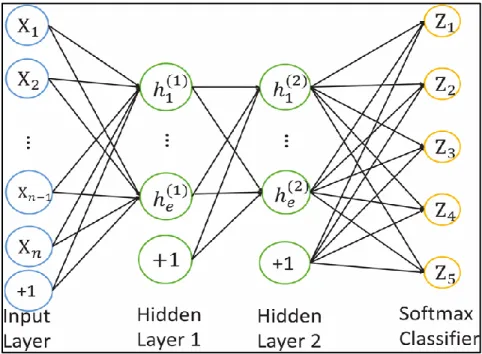
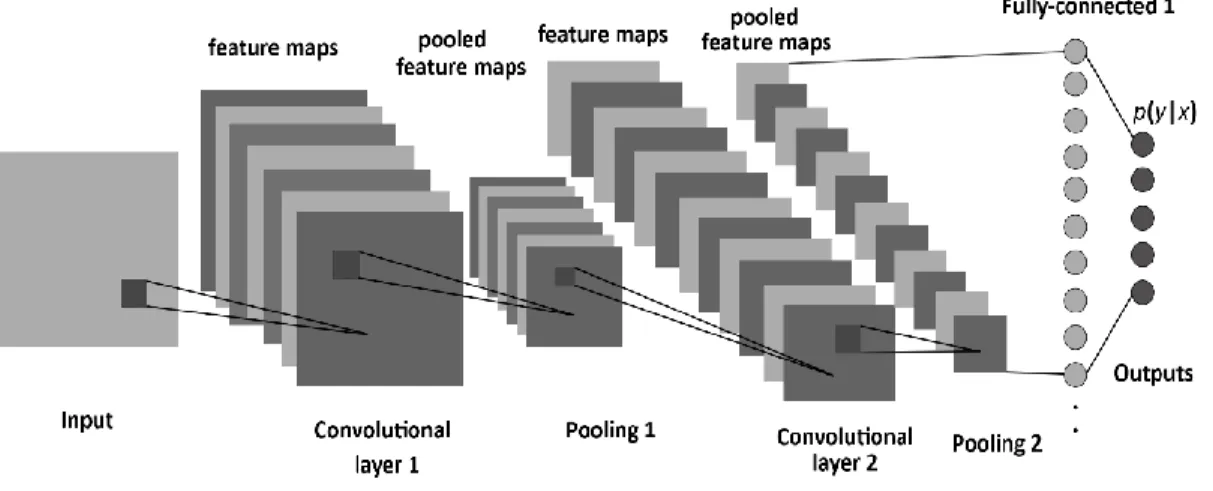
CNN is a subclass of neural networks that takes advantage of the spatial structure of the inputs. CNN models have a standard structure consisting of alternating convolutional layers and pooling layers (often each pooling layer is placed after a

(23)

10

convolutional layer). The last layers are a small number of fully-connected layers, and the final layer is a softmax classifier as shown in Figure 2.1.

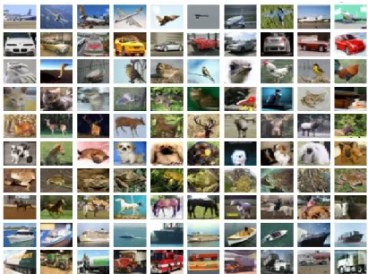
The critical advantage of CNNs is that it is trained end-to-end from raw pixels to classifier outputs to learn feature representation automatically without depending totally on human-crafted features [10, 11]. Since 2012, many researches have improved the performance of CNNs in different directions, e.g. layer design, activation function, and regularization, or applying CNNs in other areas [12, 13]. CNNs have been implemented using large data sets such as MNIST [33], CIFAR-10/100 [34], and ImageNet [35] for image recognition.

Figure 2.1. The standard structure of a CNN.

2.3.1 Convolutional Layers

The convolutional layer is comprised of a set of learnable kernels or filters which aim to extract local features from the input. Each kernel is used to calculate a feature map. The units of the feature maps can only connect to a small region of the input, called the

(24)

11

receptive field. A new feature map is typically generated by sliding a filter over the input and computing the dot product (which is similar to the convolution operation), followed by a non-linear activation function as shown in Equation 2.5 to introduce non-linearity into the model.

𝑥_𝑓(𝑙)= 𝑓 (∑ 𝑥(𝑙−1) 𝐹,𝐹

∗ 𝑤_𝑓(𝑙)+ 𝑏_𝑓(𝑙)) (2.5)

where * is convolution operation ,𝑤_𝑓(𝑙) is convolution filter with size 𝐹 × 𝐹,

𝑥(𝑙−1)_{is the output of previous layer ,} l j

b is shared bias of the feature map, and f is non-linear activation function.

During the backward phase, we compute the gradient of the loss function with respect to the weights (𝑤) and biases (𝑏) of the respective layer as follows:

∇_𝑤 𝑓(𝑙)ℓ = ∑ (∇𝐹,𝐹 𝑥𝑓(𝑙+1)ℓ)𝐹,𝐹 (𝑥𝐹,𝐹 (𝑙)_{∗ 𝑤} 𝑓(𝑙) (2.6) ∇_𝑏 𝑓(𝑙)ℓ = ∑(∇𝑥𝑓(𝑙+1) 𝐹,𝐹 ℓ)𝐹,𝐹 (𝑥𝐹,𝐹(𝑙) ∗ 𝑏𝑓(𝑙)) (2.7) All units share the same weights (filters) among each feature map. The advantage of sharing weights is the reduced number of parameters and the ability to detect the same feature, regardless of its location in the inputs [36].

Several nonlinear activation functions are available, such as sigmoid, tanh, and ReLU. However, ReLU [f(x) = max (0, x)] is preferable because it makes training faster relative to the others [1, 37]. The size of the output feature map is based on the filter size

(25)

12

and stride, so when we convolve the input image with a size of (H × H) over a filter with a size of (F × F) and a stride of (S), then the output size of (W × W) is given by:

𝑊 = ⌊𝐻 − 𝐹_𝑆 ⌋ + 1 (2.8)

The hyperparameters of each convolutional layer are filter size, the number of learnable filters, and stride. These hyperparameters must be chosen carefully in order to generate desired outputs.

2.3.2 Pooling Layers

The pooling, or down-sampling layer, reduces the resolution of the previous feature maps. Pooling produces invariance to a small transformation and/or distortion. Pooling splits the inputs into disjoint regions with a size of (R × R) to produce one output from each region [38]. Pooling can be max or average based. If a given input with a size of (W × W) is fed to the pooling layer, then the output size will be obtained by:

𝑃 = ⌊W _𝑅⌋ _(2.9)

During the forward phase, the maximum value of non-overlapping blocks from the previous feature map 𝑥(𝑙−1)_{is calculated as follows:}

𝑥(𝑙)_{= 𝑚𝑎𝑥}

𝑅,𝑅 (𝑥(𝑙−1))𝑅,𝑅 (2.10)

Max pooling does not have any learnable parameters. During the backward phase, the gradient from the next layer is passed back only to the neuron that achieved the max

(26)

13

value; all of the other neurons receive zero gradient.

2.3.3 Fully-connected Layers

The top layers of CNNs are one or more fully-connected layers similar to a feed-forward neural network, which aims to extract the global features of the inputs. Units of these layers are connected to all of the hidden units in the preceding layer. The outputs of the fully-connected layer are computed as shown in Equation 2.11:

𝑥(𝑙)_{= 𝑓((𝑤}(𝑙)₎𝑇_{∙ 𝑥}(𝑙−1)_{+ 𝑏}(𝑙)₎

(2.11)

where ∙ is a dot product , 𝑥(𝑙−1)_{is the output of the previous layer,}_𝑥(𝑙)_{, 𝑤}(𝑙)_,

and 𝑏(𝑙)_{denotes the activations, weights, and biases of the current layer}_(𝑙)_{respectively,}

and 𝑓 is the non-linear activation function.

During the backward phase, the gradient is calculated with respect to the weights and biases as follows:

∇_𝑤(𝑙)ℓ = (𝑥(𝑙))𝑇 (∇_𝑥(𝑙+1) ℓ)

(2.12)

∇_𝑏(𝑙)ℓ = (𝑥(𝑙))𝑇 (∇_𝑥(𝑙+1) ℓ) (2.13)

where ∇_𝑥(𝑙+1) is the gradient of the next higher layer.

The fully-connected layer has only one hyperparameter, which is the number of neurons (the number of learnable parameters connecting the input to the output).

(27)

14

each class label over K classes as shown in Equation (2.14) [27].

𝑦_𝑖 = exp (−𝑧𝑖)

∑𝐾𝑗=1exp (𝑧𝑗) (2.14)

2.4 CNN Architecture Design

In this dissertation, our learning algorithm for the CNN (Λ) is specified by a structural hyperparameter  which encapsulates the design of the CNN architecture as follows: 𝜆 = ((𝜆₁𝑖_{, 𝜆} 2 𝑖_{, 𝜆} 3 𝑖_{, , 𝜆} 4 𝑖₎ 𝑖=1,𝑀𝑐, (𝜆1 𝑗₎ 𝑗=1,𝑁𝑓) (2.15) where  defines the domain for each hyperparameter, (𝑀𝐶) is the number of

convolutional layers, and (𝑁_𝐹) is the number of fully-connected layers (i.e., the depth =

𝑀_𝐶+ 𝑁_𝑓). Constructing any convolutional layer requires four hyperparameters that must be identified. For example, for convolutional layer i: 𝜆₁𝑖 _{is the number of filters,}_𝜆

2 𝑖 _{is the}

filter size (receptive field size), and 𝜆₃𝑖_{defines the pooling locations and sizes. If}_𝜆 3 𝑖_is

equal to one, this means there is no pooling layer placed after convolutional layer i; otherwise, there is a pooling layer after convolutional layer i and the value 𝜆₃𝑖_{defines the}

pooling region size. 𝜆₄𝑖_{is stride step.}_𝜆 5

𝑗_{is the number of units in fully-connected layer}_j_.

We also use ℓ(Λ, 𝑇𝑇𝑅, 𝑇𝑉) to refer to the validation loss (e.g., classification error) obtained

when we train model Λwith the training set (𝑇𝑇𝑅) and evaluate it on the validation set

(28)

15

hyperparameters * that designs the architecture for a given dataset automatically, resulting in a minimization of the classification error as follows:

∗_{= 𝑎𝑟𝑔𝑚𝑖𝑛 ℓ(Λ, 𝑇}

𝑇𝑅, 𝑇𝑉) (2.16)

We define the most important hyperparameters in designing a CNN architecture below:

Depth: defines the number of convolutional layers (𝑀𝐶) and the number of

fully-connected layers 𝑁(_𝑓). So the depth= (𝑀_𝐶 + 𝑁_𝑓).

Filter size: The height and width of each filter. Generally, the sizes of the filters are quadratic, i.e. have the same width and height.

Number of filters: defines output volume and controls the number of learnable filters connected to the same region of the input volume. Each filter detects a different feature in the input.

Stride: step-size that the filter must be moved.

Pooling layer location: this defines whether the current convolutional layer is followed by a pooling layer.

Pooling region size: The amount of down-sampling to be performed. In current deep learning frameworks such as Keras and Tensorflow, the hyperparameters of the pooling layer are filter size and stride. In our work, the pooling region size is equivalent to the filter size, and we always assume that the stride is equal to the filter size, which means the pooling is always non-overlapped.

(29)

16

2.4.1 Literature Review on CNNN Architecture Design

A simple technique for selecting a CNN architecture is cross-validation [39], which runs multiple architectures and selects the best one based on its performance on the validation set. However, cross-validation can only guarantee the selection of the best architecture amongst architectures that are composed manually through a large number of choices. The most popular strategy for hyperparameter optimization is an exhaustive grid search, which tries all possible combinations through a manually-defined range for each hyperparameter. The drawback of a grid search is its expensive computation, which increases exponentially with the number of hyperparameters and the depth of exploration desired [40]. Recently, random search [41], which selects hyperparameters randomly in a defined search space, has reported better results than grid search and requires less computation time. However, neither random nor grid search use previous evaluations to select the next set of hyperparameters for testing to improve upon the desired architecture.

Recently, Bayesian Optimization (BO) methods have been used for hyperparameter optimization [21, 42, 43]. BO constructs a probabilistic model ℳ based on the previous evolutions of the objective function f. Popular techniques that implement BO are Spearmint [21], which uses a Gaussian process model for ℳ, and Sequential Model-based Algorithm Configuration (SMAC) [42], based on a random forest of the Gaussian process. According to [44], BO methods are limited because they work poorly when high-dimensional hyperparameters are involved and are very computationally expensive. The work in [21] used BO with a Gaussian process to optimize nine hyperparameters of a CNN, including the learning rate, epoch, initial weights of the

(30)

17

convolutional and full-connected layers, and the response contrast normalization parameters. Many of these hyperparameters are continuous and related to regularization, but not to the CNN architecture. Similarly, Ref. [24, 45, 46] optimized continuous hyperparameters of deep neural networks. However, Ref. [46-51] proposed many adaptive techniques for automatically updating continuous hyperparameters, such as the learning rate momentum and weight decay for each iteration to improve the coverage speed of backpropagation. In addition, early stopping [52, 53] can be used when the error rate on a validation set or training set has not improved, or when the error rate increases for a number of epochs. In [54], an effective technique is proposed to initialize the weights of convolutional and fully-connected layers.

Evolutionary algorithms are widely used to automate the architecture design of learning algorithms. In [25], a genetic algorithm is used to optimize the filter sizes and the number of filters in the convolutional layers. Their architectures consisted of three convolutional layers and one fully-connected layer. Since several hyperparameters were not optimized, such as depth, pooling regions and sizes, the error rate was high, around 25%. Particle Swarm Optimization (PSO) is used to optimize the feed-forward neural network’s architecture design [55].Soft computing techniques are used to solve different real applications, such as rainfall and forecasting prediction [56, 57]. PSO is widely used for optimizing rainfall–runoff modeling. For example, Ref. [58] utilized PSO as well as extreme learning machines in the selection of data-driven input variables. Similarly, [59] used PSO for multiple ensemble pruning. However, the drawback of evolutionary algorithms is that the computation cost is very high, since each population member or

(31)

18

particle is an instance of a CNN architecture, and each one must be trained, adjusted and evaluated in each iteration. In [60], ℓ1 Regularization is used to automate the selection of

the number of units only for fully-connected layers for artificial neural networks.

Recently, interest in architecture design for deep learning has increased. The proposed work in [61] applied reinforcement learning and recurrent neural networks to explore architectures, which have shown impressive results. Ref. [62] proposed a CoDeepNEAT-based Neuron Evolution of Augmenting Topologies (NEAT) to determine the type of each layer and its hyperparameters. Ref. [63] used a genetic algorithm to design a complex CNN architecture through mutation operations and managing problems in filter sizes through zeroth order interpolation. Each experiment was distributed to over 250 parallel workers to find the best architecture. Reinforcement learning, based on Q-learning [64], was used to search the architecture design by discovering one layer at a time, where the depth is decided by the user. However, these promising results were achieved only with significant computational resources and a long execution time.

Visualization approach in [14, 65] is another technique used to visualize feature maps to monitor the evolution of features during training and thus discover problems in a trained CNN. As a result, the work presented in [14] visualized the second layer of the AlexNet model, which showed aliasing artifacts. They improved its performance by reducing the stride and kernel size in the first layer. However, potential problems in the CNN architecture are diagnosed manually, which requires expert knowledge. The selection of a new CNN architecture is then done manually as well.

(32)

19

2.5 Regularization

In CNNs, overfitting is a major problem, which regularization can effectively reduce. There are several techniques to combat this problem, including L1, L2 weight decay, KL-sparsity, early stopping, data augmentation, and dropout. Dropout has proven itself an effective method to reduce overfitting due to its ability to provide a better generalization on the testing set. Because dropout is such a powerful technique, it has encouraged recent success in CNNs

Dropout [11] is a powerful technique for regularizing full connected layers within neural networks or CNN. The idea of dropout is each neuron is selected randomly with probability p to be dropped (setting the activation to zero) for each training case. This helps to prevent hidden neurons from co-adapting with each other too much; forcing the model based on a subset of hidden neurons. The error back-propagated through only remaining neurons that are not dropped. On the other hand, we can look to the dropout as model averaging of large number of neural network models.

Early stopping [52, 53] is a kind of regularization that helps to avoid overfitting by monitoring the performance of the model on the validation set. Once the performance on the validation dataset decreases or saturates for a number of iterations, the model stops the training procedure.

2.6 Weight initialization

Weight initialization [18] is a critical step in CNNs that influences the training process. In order to initialize the model’s parameters properly, the weights must be within

(33)

20

a reasonable range before the training process begins. As a result, this will make the convergence faster. Several weight initialization methods have been proposed, including random initialization, naive initialization, and Xavier initialization. The two most widely used are naive initialization and Xavier initialization.

 Naive initialization, the weights are initialized from a Gaussian distribution with a mean of zero and a small value of standard deviation.

 Xavier initialization [54] has become the default technique for weight initialization in CNNs. It tries to keep the variance between the layers approximately the same. The advantage of Xavier initialization is that it makes the network converge much faster than other approaches. The weight sets it produces are also more consistent than those produced by other techniques.

2.7 Visualizing and Understanding CNNs

There are three main methods for understanding and visualizing CNNs as follows:  Layer activations: this simple technique shows the activations of a network

during the forward pass. The drawback, however, is that some activation maps’ outputs are zero for the input images, which indicates dead filters. Additionally, the size of the activation maps is not equal to the input image, especially in higher layers.

 Retrieving images that maximally activate a neuron: this strategy feeds a large set of images through the network and then keeps track of which images maximize the activations of the neurons. However, the limitation of this technique is that the

(34)

21

ReLU activation function does not always have semantic meaning by itself. This method can involve a high computational cost to find the images that maximize the neurons’ values [66].

 Deconvolutional networks: aims to project the learned features in higher layers down to the input pixel space for a trained CNN. This results in a reconstructed image the same size as the input image. It contains the regions of the input image that were learned by a given feature map. A visualization similar to the input image indicates that the CNN architecture learned properly. Since the reconstructed image is the same size as the input, this allows us to measure the similarity between the inputs and their reconstruction effectively [67] (Details in 5.3)

2.8 Similarity Measurements between Images

Several methods are used to compare the similarity between two images or vectors. The most widely used are Euclidean distance, mutual information, and a correlation coefficient. Each one of these methods has advantages and disadvantages.

 The Euclidean distance between two images is the sum of the squared intensity differences of corresponding pixels in sequences as shown in Equation 2.17. The drawback of Euclidean distance is that it is very sensitive to normalization of the data, so any tiny errors will produce inaccurate results. Euclidean distance between two vectors q and p is computed by:

(35)

22

𝑑(𝑝, 𝑞) = √∑(𝑝_𝑖

𝑦 𝑖=1

− 𝑞_𝑖)2_ (2.17)

 Mutual information is a concept derived from information theory. The mutual information measures the dependencies between two images, or the amount of information that one image contains about the other. The value of mutual information will be large when the similarity between a pair of images is high. Mutual information denoted as 𝑀𝐼(𝑋, 𝑌) between two grayscale images 𝑋 and 𝑌 is given by: 𝑀𝐼(𝑋, 𝑌) = ∑ ∑ 𝑝(𝑥, 𝑦)𝑙𝑜𝑔 𝑝(𝑥, 𝑦) 𝑝(𝑥)𝑝(𝑦) 255 𝑦=0 255 𝑥=0 (2.18)

where p(x) and p(y) are marginal distributions of 𝑋, 𝑌 respectively, and p(x, y) is a joint probability distribution. The key advantage of mutual information is that it detects the non-linear dependence between two images. The drawback of mutual information is that it is computationally very expensive [68].

 Correlation distance is the linear dependence between two images. Fast Fourier Transform (FFT) provides another approach to calculate the correlation coefficient with a high computational speed as compared to the original correlation coefficient formula and mutual information (further detail is provided in Chapter 3.1.3).

2.9 Sparse Autoencoder

(36)

23

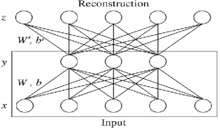
identical function 𝑓(𝑥) = 𝑥 by making the target outputs equal to the inputs during the training phase. SA applies backpropagation to learn meaningful features from unlabeled data. SA includes encoder and decoder steps. The encoder takes the input vector x to the hidden layer representation y with a non-linear activation function, such as sigmoid 𝑓, as shown in the following equation:

𝑦 = 𝑓(𝑊𝑥 + 𝑏) (2.19)

The decoder maps the hidden representation y back into reconstruction 𝑧 of the same input vector 𝑥 as shown inFigure 2.2.

𝑦 = 𝑓(𝑊′_{𝑦 + 𝑏) ≃ 𝑥} _(2.20)

SA is trained by back-propagation usually via gradient descent to reduce the average reconstruction error 𝐿(𝑧, 𝑥) = ||𝑧 − 𝑥||2_._{SA imposes sparsity on many hidden}

neurons’ outputs to make them zero or close to zero in order to discover interesting an feature representation and removing redundant and noisy information from the inputs [69].

Therefore, the cost function of sparse autoencoder is obtained by:

(𝑊, 𝑏) = 1 2𝑚∑ ∥ 𝑥(𝑖) 𝑛 𝑖=1 − 𝑧(𝑖)∥2₊𝜆 2∥ 𝑊 ∥ +𝛽 ∑ 𝐾𝐿(𝜌 ∥ 𝑠 𝑗=1 𝜌 ̂ ) _(2.21)

The first term of cost function in Equation 2.11 is an average sum of squares error which describes the discrepancyerror between the inputs x(i)_{and its reconstruction}_z(i) over the entire training samples. The second term is weight decay, which is a regularization technique for preventing overfitting. The last term is an extra penalty term

(37)

24

to provide sparsity constraint, where 𝜌 is the sparsity parameter and typically takes a small value, n is number of neurons in the hidden layer, and the index j sums over the hidden neurons in our network. A 𝐾𝐿(𝜌𝜌̂) is a Kullback-Leibler (KL) divergence between 𝜌̂ which is an average activation (averaged over the training data) of hidden neuron j, and the target activations 𝜌_𝑖 which can be defined as:

𝐾𝐿(𝜌||𝜌̂𝑗) = 𝜌 𝑙𝑜𝑔

𝜌

𝜌̂_𝑗+ (1 − 𝜌) log 1 − 𝜌

1 − 𝜌̂_𝑗 (2.22)

where 𝜌 is a sparsity parameter, typically a small value close to zero (say 𝜌 = 0.05). Therefore, we would like the average activation of each hidden neuron 𝑗 to be close to 0.05. To satisfy this constraint, the hidden unit’s activations must mostly be near zero.

Figure 2.2. Sparse Autoencoder structure: The number of units in input layer is equal to number of units in output layer.

2.10 Analysis of optimized instance selection algorithms on large

datasets with CNNs

It is common that training set consists of instances that are useless. Therefore, it is probable to get acceptable performance and enhance the training execution time

(38)

25

without non-useful instances; this process is called instance selection [70, 71].

Instance selection aims to choose subset (𝑇𝑆) from training set (𝑇𝑇𝑅) where

( 𝑇_𝑆 ⊂ 𝑇_𝑇𝑅) to accomplish the original task of classification application with little or no performance degradation as if the entire training set (𝑇_𝑇𝑅) is used. This training set might contain superfluous instances which can be redundant or noisy. Removing these instances is required because they may cause performance deterioration [72]. Furthermore, reducing the training set will shrink the amount of computation and memory storage, especially if the amount of training set is large with high dimensionality. Each instance in a training set can be either border instance or interior instance. Border instance is its k

nearest neighbors (k-NN) belonging to other classes that usually are closer to the decision boundary. Interior instance is its k nearest neighbors belonging to the same class [73].

Instance selection can be divided into three types of algorithms: condensation, edition, and hybrid [74]. Condensation techniques aim to retain border instances. This leads to make the accuracy over training set high but it might reduce the generalization accuracy over the testing set. The reduction rate is high in condensation methods [75]. Edition methods aim to discard the border instances and retain interior instances. Consequently, this leads to a smoother decision boundary between classes, which can improve the classifier accuracy over the testing set. Finally, hybrid methods seek to choose a subset of the training set containing border and interior instances to maintain or enhance the generalization accuracy.

An instance selection search can be incremental, decremental or mixed. Incremental methods start with empty subset 𝑇𝑆=, and add each instance to 𝑇𝑆 from 𝑇𝑇𝑅

(39)

26

if it qualifies for some criteria. Decremental search starts with 𝑇_𝑆=𝑇_𝑇𝑅and removes any instance 𝐼𝑖𝑚𝑔from 𝑇𝑆 if it does not fulfill specific criteria. Mixed search starts with

pre-selected subset 𝑇_𝑆 and iteratively can add or remove any instance meet the specific criteria [71, 74].

All instance selection methods work under the following assumption: 𝑇𝑇𝑅 is the

training set; 𝐼_{𝑖𝑚𝑔_𝑖} is i-th instance in 𝑇_𝑇𝑅. Subset 𝑇_𝑆 is selected from 𝑇_𝑇𝑅; 𝐼_{𝑖𝑚𝑔_𝑗}is j-th

instance in 𝑇_𝑆. 𝑇_𝑉 is the validation set. 𝑇_𝑇𝑆 is the testing set. Typically, the accuracy of instance selection methods is determined by k Nearest Neighbors (k-NN) [76]. The Euclidean distance function is used to calculate the similarity between two instances q

and p as shown in Equation 2.17.

2.10.1 Literature Review for Instance Selection

Condensed Nearest Neighbor (ConNN) [77] was first algorithm of instance selection. The algorithm is an incremental method that starts with adding one instance of each class to the subset 𝑇𝑆 randomly from training set 𝑇𝑇𝑅. Then, for each instance 𝐼𝑖𝑚𝑔

in 𝑇_𝑇𝑅 is classified using the instances in 𝑇_𝑆. If the instance 𝐼_𝑖𝑚𝑔 is incorrectly classified, it will be added to 𝑇_𝑆. This guarantees all instances in 𝑇_𝑇𝑅 are classified correctly. Based on this criterion, noisy instance will be retained because they are commonly classified wrongly by their k-NN.

The Edited Nearest Neighbor (ENN) [78] algorithm starts with 𝑇_𝑆 =𝑇_𝑇𝑅, and then each instance 𝐼𝑖𝑚𝑔 in 𝑇𝑆 is removed from 𝑇𝑆 if it does not agree with the majority of k-NN

(40)

27

(e.g. k=3). The ENN discards noisy instances as well as border instances to yield smooth boundaries between classes by saving interior instances.

All k-NN [79] belongs to the family of ENN. The algorithm works as follows: for

i=1 to k, flags as bad for each instance misclassified by its k-NN. Once the loop is ended, it discards any instance from 𝑇_𝑆 if it is flagged as bad.

Skalak [80] exploited Random Mutation Hill Climbing (RMHC) method [81] to select the subset 𝑇𝑆 from 𝑇𝑇𝑅. This algorithm has two parameters should be defined by

the user early: (1) 𝑁𝑆 is the size of the subset or the training sample 𝑇𝑆. (2) 𝑁𝑖𝑡𝑒𝑟 is number

of iterations. The algorithm is based on coding instances in 𝑇_𝑇𝑅 into binary string format. Each bit represents one instance, where 𝑁_𝑆 bits are equal to one randomly (they represent 𝑇_𝑆). For 𝑁_{𝑖𝑡𝑒𝑟}iterations, the algorithm randomly mutates a single bit of zero to one. The accuracy will be computed, if the change increases the accuracy, the change will be kept, otherwise, roll-backed. This algorithm gives high chance to increase the size of

𝑇𝑆 with increasing iteration

In [74] explained RMHC in a different way as follows: the algorithm begins to select 𝑁_𝑆instances randomly from 𝑇_𝑇𝑅 to represent 𝑇_𝑆. For 𝑁_{𝑖𝑡𝑒𝑟} iterations: the algorithm replaces one instance selected randomly from 𝑇_𝑆 with instance selected randomly from (𝑇𝑇𝑅-𝑇𝑆). If the change improves the accuracy on the testing data using 1-NN, the change

will be maintained, otherwise, the change will be roll-backed. The size of 𝑇𝑆 in this way

(41)

28

2.11 A Deep Architecture for Face Recognition Based on Multiple

Feature Extractors

In recent decades, face recognition has been widely explored in the areas of computer vision and image analysis due to its numerous application domains such as surveillance, smart cards, law enforcement, access control, and information security. With the number of face recognition algorithms that have been developed, face recognition is still a very challenging task with respect to the changes in facial expression, illumination, background and pose [82].

The performance of each individual classifier has shown sensitivity to some changes in facial appearance. Combining Multiple Classifiers (MC) in one system has become a new direction which integrates many information resources and is likely enhance the performance. The combination of MC can be applied at two levels: the decision level and the feature level. The decision level addresses how to combine the outputs of MC. In the feature level, each classifier produces a new representation that will be concatenated in a feature vector to be fed into the new classifier [83]. This is the approach we follow in our work. MC is only useful if combined classifiers are mutually complementary, and they do not make coincident errors [84]. MC is a very effective solution for classification problems involving a lot of classes and noisy input data [85].

In general, an MC system has three main topologies: parallel, serial and hybrid [86]. The design of an MC system consists of two main steps: the classifier ensemble and fuser. The classifier ensemble defines the selection of combined classifiers to be most effective. The fuser step combines the results that are obtained by each individual

(42)

29

classifier [87]. The final classification can be greatly improved using deep learning. In this dissertation, we also employ the power of combining MC and deep learning to build a system that uses different feature extraction algorithms, namely PCA, LBP+PCA, and LBP+NN, to ensure that each classifier produces its own basis representation in a meaningful way. We then form a joint feature vector by concatenating the outputs of the above three MCs. This joint feature vector is then fed into a deep SA with two hidden layers to generate the classification results with probabilistic distribution to approximate the probability of each class label. We present the results of a series of experiments for different existing MC systems, replacing different classifiers with SSA, to exhibit the efficiency of deep SSA classification as compared to other classifiers implementation.

2.11.1 Literature Review for Multiple Classifiers

Lu et al [88] combined the basis vectors of PCA, ICA and LDA. The authors used sum rule as well as RBF network strategies to integrate the outputs of three classifiers, using matching scores. The outputs of the classifiers are concatenated into one vector to be used as input to the RBF network to get the final decision. All feature extractors used in this system are holistic techniques which utilize the information of the entire face to be projected into subspace. The drawback of this approach is that the classification results (not features) are combined from each classifier, whereas in this work, we combine the individual features from different classifiers in a balanced way into a deep learning based final classifier. Thus, preserving the entire feature information from an individual

(43)

30 classifier until the final result is produced.

Lawrence et al [89] proposed a hybrid neural network comprising of local image sampling, a self-organizing map (SOM) neural network and convolution neural networks (CNN). SOM is used for reducing dimensionality and invariance to small changes in the images. CNN provides partial distortion invariance. Replacing SOM by the Karhunen-Loeve transform produced a slightly worse result. While this approach produces good results and to some extent is invariant to small changes in the input image, the classification depends only on features obtained from dimensionality reduction. The best reported result on the ORL dataset was 96.2%, whereas the approach in this work which relies on diverse features from different techniques (including dimensionality reduction) achieves an accuracy of 98% on the ORL database.

Eleyan and Demirel [90] proposed two systems for face recognition; PCA followed by neural network (NN) and LDA followed by (NN). PCA and LDA are used for dimensionality reduction to be fed into NN for classification. LDA+ NN outperforms PCA+NN.

Lone et al [91] developed a single system for face recognition that combines four individual algorithms namely PCA, Discrete Cosine Transform (DCT), Template Matching using correlation (Corr) and Partitioned Iterative Function System (PIFS). In addition, they compared the results by combining two techniques of PCA-DCT, and three techniques based on PCA-DCT-Corr. The results show that combining four Algorithms outperforms combination of two as well as three Algorithms. They obtained 86.8% accuracy rate on ORL database.

(44)

31

Liong et al [92] proposed a new technique, called deep PCA, to obtain a deep representation of data, which will be discriminant and better for recognition. The approach comprises of two layers which are whitening and PCA. The outputs of first layer will be inserted into the second layer to perform whitening and PCA again.

(45)

32

CHAPTER 3: RESEARCH PLAN

3.1 A Framework for Designing the Architectures of Deep CNNs

In existing approaches to hyperparameter optimization and model selection, the dominant approach to evaluating multiple models is the minimization of the error rate on the validation set. In this work, we describe a better approach based on introducing a new objective function that exploits the error rate as well as the visualization results from feature activations via deconvnet. Another advantage of our objective function is that it does not get stuck easily in local minima during optimization using NMM. Our approach obtains a final architecture that outperforms others that use the error rate objective function alone.

In this section, we present information on the framework model consisting of deconvolutional networks, the correlation coefficient, and the objective function. NMM guides the CNN architecture by minimizing the proposed objective function, and web services help to obtain a high-performing CNN architecture for a given dataset. For large datasets, we use instance selection and statistics to determine the optimal, reduced training dataset as a preprocessing step. A general framework flowchart and components are shown in Figure 3.1. In order to accelerate the optimization process, we employ multiple techniques, including training on an optimized dataset, parallel and distributed execution, and correlation coefficient computation via FFT.

(46)

33

Figure 3.1. General components and a flowchart of our framework for discovering a high-performing CNN architecture

3.1.1 Reducing the Training Set

Training deep CNN architectures with a large training set involves a high computational time. The large dataset may contain redundant or useless images. In

(47)

34

machine learning, a common approach of dealing with a large dataset is instance selection, which aims to choose a subset or sample (𝑇𝑆) of the training set (𝑇𝑇𝑅) to

achieve acceptable accuracy as if the whole training set was being used. Many instance selection algorithms have been proposed and reviewed in [71]. Albelwi and Mahmood [76] evaluated and analyzed the performance of different instance selection algorithms on CNNs. In this framework, for very large datasets, we employ instance selection based on Random Mutual Hill Climbing (RMHC) [80]as a preprocessing step to select the training sample (𝑇_𝑆) which will be used during the exploration phase to find a high-performing architecture. The reason for selecting RMHC is that the user can predefine the size of the training sample, which is not possible with other algorithms. We employ statistics to determine the most representative sample size, which is critical to obtaining accurate results.

In statistics, calculating the optimal size of a sample depends on two main factors: the margin of error and confidence level. The margin of error defines the maximum range of error between the results of the whole population (training set) and the result of a sample (training sample). The confidence level measures the reliability of the results of the training sample, which reflects the training set. Typical confidence level values are 90%, 95%, or 99%. We use a 95% confidence interval in determining the optimal size of a training sample (based on RHMC) to represent the whole training set.

3.1.2 CNN Feature Visualization Methods

(48)

35

explore the inner operations of a CNN, which enables us to understand what the neurons have learned. There are several visualization approaches. A simple technique called layer activation shows the activations of the feature maps [93] as a bitmap. However, to trace what has been detected in a CNN is very difficult. Another technique is activation maximization [94], which retrieves the images that maximally activate the neuron. The limitation of this method is that the ReLU activation function does not always have a semantic meaning by itself. Another technique is deconvolutional network [14], which shows the parts of the input image that are learned by a given feature map. The deconvolutional approach is selected in our work because it results in a more meaningful visualization and also allows us to diagnose potential problems with the architecture design.

3.1.2.1Deconvolutional Networks

Deconvolutional networks (deconvnet) [14] are designed to map the activities of a given feature in higher layers to go back into the input space of a trained CNN. The output of deconvnet is a reconstructed image that displays the activated parts of the input image learned by a given feature map. Visualization is useful for evaluating the behavior of a trained architecture because a good visualization indicates that a CNN is learning properly, whereas a poor visualization shows ineffective learning. Thus, it can help tune the CNN architecture design accordingly in order to enhance its performance. We attach a deconvnet layer with each convolutional layer similar to [14], as illustrated at the top of Figure 3.2. Deconvnet applies the same operations of a CNN but in reverse, including unpooling, a non-linear activation function (in our framework, ReLU), and filtering.

(49)

36

Figure 3.2. The top part illustrates the deconvnet layer on the left, attached to the convolutional layer on the right. The bottom part illustrates the pooling and unpooling operations [14].

The deconvnet process involves a standard forward pass through the CNN layers until it reaches the desired layer that contains the selected feature map to be visualized. In a max pooling operation, it is important to record the locations of the maxima of each pooling region in switch variables because max pooling is non-invertible. All feature maps in a desired layer will be set to zero except the one that is to be visualized. Now we can use deconvnet operations to go back to the input space for performing reconstruction. Unpooling aims to reconstruct the original size of the activations by using switch variables to return the activation from the layer above to its original position in the pooling layer, as shown at the bottom of Figure 3.2, thereby preserving the structure of the stimulus. Then, the output of the unpooling passes through the ReLU function. Finally, deconvnet applies a convolution operation on the rectified, unpooled maps with

(50)

37

transposed filters in the corresponding convolutional layer. Consequently, the result of deconvnet is a reconstructed image that contains the activated pieces of the input that were learnt. Figure 3.3 displays the visualization of different CNN architectures. As shown, the quality of the visualization varies from one architecture to another compared to the original images in grayscale. For example, CNN architecture 1 shows very good visualization; this gives a positive indication about the architecture design. On the other hand, CNN architecture 3 shows poor visualization, indicating this architecture has potential problems and did not learn properly.

The visualization of feature maps is thus useful in diagnosing potential problems in CNN architectures. This helps in modifying an architecture to enhance its performance, and also evaluating different architectures with criteria besides the classification error on the validation set. Once the reconstructed image is obtained, we use the correlation coefficient to measure the similarity between the input image and its reconstructed image in order to evaluate the reconstruction’s representation quality.

Figure 3.3. Visualization from the last convolutional layer for three different CNN architectures. Grayscale input images are visualized after preprocessing.

(51)

38

3.1.3 Correlation Coefficient

The correlation coefficient (Corr) [95] measures the level of similarity between two images or independent variables. The correlation coefficient is maximal when two images are highly similar. The correlation coefficient between two images A and B is given by: 𝐶𝑜𝑟𝑟(𝐴, 𝐵) =1 𝑛∑( 𝑎_𝑖− 𝑎̅ 𝜎𝑎 ) 𝑛 𝑖=1 (𝑏𝑖− 𝑏̅ 𝜎𝑏 ) (3.1)

where 𝑎̅ and 𝑏̅ are the averages of A and B respectively, 𝜎_𝑎 denotes the standard deviation of A, and 𝜎𝑏 denotes the standard deviation of B. Fast Fourier Transform (FFT)

provides an alternative approach to calculate the correlation coefficient with a high computational speed as compared to Equation (3.1) [96, 97]. The correlation coefficient between A and B is computed by locating the maximum value of the following equation:

𝐶𝑜𝑟𝑟(𝐴, 𝐵) = ℱ−1_{[ℱ(𝐴) ∘ ℱ}∗_(𝐵)] _(3.2)

where ℱ is an FFT for a two-dimensional image, ℱ−1_{indicates inverse FFT, * is}

the complex conjugate, and ∘ implies element by element multiplication. This approach reduces the time complexity of the computing correlation from 𝑂(𝑁2₎_to_{𝑂(𝑁 log 𝑁)}_.

Once the training of the CNN is complete, we compute the error rate (Err) on the validation set, and choose Nfm feature maps at random from the last layer to visualize their learned parts using deconvnet. The motivation behind selecting the last convolutional layer is that it should show the highest level of visualization as compared to preceding layers. We choose Nimg images from the training sample at random to test the deconvnet.