Anthropology Theses Department of Anthropology
Summer 8-8-2017
A MORPHOMETRIC STUDY OF
MAXILLARY POST CANINE DENTITION IN
AUSTRALOPITHECUS AFRICANUS FROM
STERKFONTEIN, SOUTH AFRICA: ONE
SPECIES OR TWO?
Lesley K. Mackie
Colorado College
Follow this and additional works at:https://scholarworks.gsu.edu/anthro_theses
This Thesis is brought to you for free and open access by the Department of Anthropology at ScholarWorks @ Georgia State University. It has been accepted for inclusion in Anthropology Theses by an authorized administrator of ScholarWorks @ Georgia State University. For more information, please [email protected].
Recommended Citation
AUSTRALOPITHECUS AFRICANUS FROM STERKFONTEIN, SOUTH AFRICA: ONE SPECIES OR TWO?
by
LESLEY KATHLEEN MACKIE
Under the Direction of Frank L’Engle Williams, Ph.D
ABSTRACT
The objective of this study was to examine whether the premolars and molars found at Sterkfontein Sts Mbr. 4 and StW Mbr. 5 are morphometrically similar to the degree that all individuals could belong to the same species, A. africanus. Mesial-distal (MD) and buccal-lingual (BL) measurements were obtained from maxillary premolars (P3 and P4) and molars (M1, M2, and M3) of Homo, Pan, and Gorilla, and compared to their counterparts attributed to A. africanus from Sterkfontein. Specimen samples were statistically analyzed using univariate and multivariate analyses. The results support the acceptance of the null hypothesis, indicating that the dental remains from Sts Mbr. 4 and StW Mbr 5 are from the same species.
AUSTRALOPITHECUS AFRICANUS FROM STERKFONTEIN, SOUTH AFRICA: ONE SPECIES OR TWO?
by
LESLEY KATHLEEN MACKIE
A Thesis Submitted in Partial Fulfillment of the Requirements for the Degree of Master of Arts
in the College of Arts and Sciences Georgia State University
Copyright by Lesley Kathleen Mackie
AUSTRALOPITHECUS AFRICANUS FROM STERKFONTEIN, SOUTH AFRICA: ONE SPECIES OR TWO?
by
LESLEY KATHLEEN MACKIE
Committee Chair: Frank L’Engle Williams
Committee: Bethany Turner-Livermore Jeffrey B. Glover
Electronic Version Approved:
ACKNOWLEDGEMENTS
Thank you to Lauren Smith and Ben Marks at the Chicago Field Museum and to Lyman M. Jellema at the Cleveland Museum of Natural History for allowing access to their collections so that dental measurements could be collected.
Many thanks to this thesis committee for their time and for providing insight throughout this degree seeking process. Their efforts to make their classes enjoyable and educational are greatly appreciated. Dr. Williams, in particular, is thanked for agreeing to act as advisor, for his field notes and for being an invaluable source of guidance during this process.
Francis Thackeray of the Ditsong Museum of Natural History (formerly the Transvaal Museum) and Phillip Tobias (posthumously) of the University of the Witwatersrand, School of Medical are thanked for allowing Dr. Williams access to the original Australopithecus africanus
TABLE OF CONTENTS
ACKNOWLEDGEMENTS ... V
LIST OF TABLES ... IX
LIST OF FIGURES ... X
1 INTRODUCTION ... 1
1.1 Background ... 1
1.1.1 Sterkfontein ... 1
1.1.2 Stratigraphy ... 3
1.1.3 Paleoecology ... 6
1.1.4 Australopithecus africanus ... 9
1.1.5 Number of Species ... 10
1.2 Purpose of the Study ... 12
1.3 Expected Results ... 12
2 LITERATURE REVIEW ... 14
2.1 Species/Species Concepts ... 14
2.1.1 BioSpecies Concept ... 15
2.1.2 Specific Mate Recognition System Concept ... 16
2.1.3 Phylogenetic Species Concept ... 17
2.1.4 Evolutionary Concept ... 17
2.2 Primate Species ... 18
2.3 Identifying A. africanus and Other Hominin Species ... 19
2.4 Dentition ... 21
2.5 Sexual Dimorphism ... 22
2.6 Conclusion ... 23
3 METHODS ... 25
3.1 Data Collection ... 25
3.2 Measurement Error Analysis ... 27
3.3 Data Analysis ... 28
3.3.1 Descriptive Analysis ... 28
3.3.2 Univariate Analysis ... 28
3.3.3 Multivariate Analysis ... 29
4 RESULTS ... 30
4.1 Descriptive Analysis ... 30
4.1.1 Descriptive Analysis for Males ... 31
4.1.2 Descriptive Analysis for Females ... 32
4.2 Univariate Analysis ... 33
4.2.1 ANOVA and Tukey’s HSD Unscaled ... 33
4.2.2 ANOVA and Tukey’s HSD Scaled ... 37
4.3.1 Premolars Unscaled ... 39
4.3.2 Molars Unscaled ... 41
4.3.3 Premolars Scaled... 43
4.3.4 Molars Scaled ... 45
4.3.5 Cluster Analysis... 47
5 DISCUSSION ... 50
6 CONCLUSIONS ... 54
LIST OF TABLES
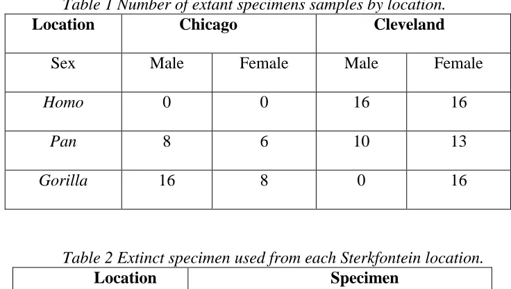
Table 1 Number of extant specimens samples by location. ... 26
Table 2 Extinct specimen used from each Sterkfontein location. ... 26
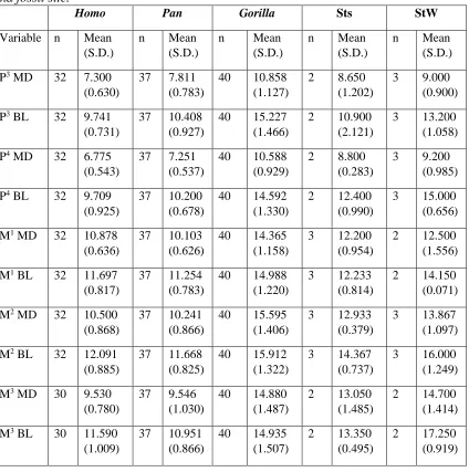
Table 3 Means (and standard deviation, S.D.) for each tooth variable for each species and fossil site. ... 31
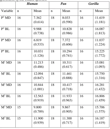
Table 4 Means (and standard deviation, S.D.) for each tooth variable for the male specimens of the extant species. ... 32
Table 5 Means (and standard deviation, S.D.) for each tooth variable for the female specimens of the extant species. ... 33
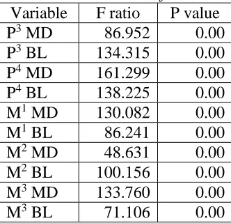
Table 6 ANOVA for each unscaled tooth variable. ... 34
Table 7 Tukey’s test results for each statistically significant species pairing by unscaled tooth variable. ... 36
Table 8 ANOVA for each scaled tooth variable. ... 38
Table 9 Tukey’s test results for each statistically significant species pairing by scaled tooth variable. ... 38
Table 10 Jackknifed classification matrix for the unscaled premolars. ... 39
Table 11 Canonical discriminant function for unscaled premolars. ... 40
Table 12 Jackknifed classification matrix for unscaled molars. ... 42
Table 13 Canonical discriminant function for unscaled molars. ... 42
Table 14 Jackknifed classification matrix for scaled premolars. ... 44
Table 15 Canonical discriminant function for scaled premolars. ... 44
Table 16 Jackknifed classification matrix for scaled molars. ... 46
LIST OF FIGURES
Figure 1 Location of Sterkfontein, South Africa. ... 2
Figure 2 Stratigraphy of the Sterkfontein Formation. ... 4
Figure 3 Scatterplot for unscaled premolars. ... 41
Figure 4 Scatterplot for unscaled molars. ... 43
Figure 5 Scatterplot for scaled premolars. ... 45
Figure 6 Scatterplot for unscaled premolars. ... 47
Figure 7 Cluster analysis of unscaled data. ... 48
1 INTRODUCTION
1.1 Background
The Sterkfontein cave system has had an active hominin history for millions of years. This site has yielded several hundred hominin specimens including early Homo, Paranthropus
and Australopithecus (Herries & Shaw, 2011). Sterkfontein has a complex stratigraphy, which provides information on the paleoecology of the area during the Plio-Pleistocene transition, and more specifically, on A. africanus.
1.1.1 Sterkfontein
Figure 1 Location of Sterkfontein, South Africa (reprinted with permission from Stratford, Grab, & Pickering, 2014).
The Sterkfontein Formation has numerous different chambers many of which are named. In general, the Sterkfontein formation is divided into eastern and western sides. The east side consists of the original area of excavation, the Type Site, and the fossils found on this side are labeled Sts (Brain, 1981; Partridge & Watt, 1991). Fossils labeled StW are from the west side, the Expansion Site, which consists of the West Pit and the Silverberg Grotto. Excavations began on the west side in the 1950’s (Brain, 1981).
1981). This resulted in the discovery, by Broom and Robinson, of a complete adult cranium, Ms. Ples (Sts 5), in 1947 (Brain, 1981). Also found that year, in Member 4, was a pelvis and
articulated vertebral column (Brain, 1981). Broom and Robinson worked this site from 1947 to 1949 before changing their focus to Swartkrans and other sites (Brain, 1981). From 1957 to 1958 Robinson returned to Sterkfontein and discovered stone tool artifacts and bone tools (Brain, 1981). Many additional specimens were collected in the 1970’s (Brain, 1981) and discoveries continue at this site to this day.
1.1.2 Stratigraphy
The Sterkfontein Formation is a complex, multi-level, multi-period system (Herries & Shaw, 2011) that extends to a depth of 30 m below the surface (Partridge & Watt, 1991). Stratigraphic relationships are complex and poorly understood which makes dating difficult. This complexity can be attributed to both human and natural forces. Human forces include the removal of materials during mining at the site, complex infilling, and sediment reworking (Granger et al., 2015). Natural forces include overlapping layers of fossiliferous breccia (Granger et al., 2015), hillside erosion (Partridge, 1978), the fluidity of deposition, ceiling collapses (Herries & Shaw, 2011), and a lack of exposed sections of the stratigraphy, which is necessary to link various fossil bearing deposits (Herries & Shaw, 2011).
The Sterkfontein Formation has an inverted age stratigraphy (Herries & Shaw, 2011), meaning that it is layered with the youngest deposits occurring at the surface (Herries & Shaw, 2011). Partridge (1978) divided the cave into 6 members, in what he thought to be the
Member 5 which has subunits A, B, and C (Herries & Shaw, 2011; Partridge, 1978). Members 1, 2, and 3 are located inside the cave, while Members 4, 5, and 6 are exposed to the surface due to roof erosion (Granger et al., 2015).
Figure 2 Stratigraphy of the Sterkfontein Formation (reprinted with permission from Pickering, Clarke, & Heaton, 2004).
Member 2 is the lowest and oldest fossil bearing layer, and is described as a deathtrap assemblage (Bruxelles, Clarke, Maire, Ortega, & Stratford, 2014). The assemblage consists mainly of primates and carnivores, with bovids being scarce (Granger et al., 2015; Bruxelles, Clarke, Maire, Ortega, & Stratford, 2014). Within the Silverberg Grotto Mbr. 2, a single
Autralopithecus has been discovered, StW 573, originally labeled as A. prometheus (Granger et al., 2015).
To date, archaeologists have been focused on Member 4 (Mbr. 4) and Member 5 (Mbr. 5) (Partridge & Watt, 1991). Member 5 has been dated at 2.0 to 1.5 million years ago (Mya)
(Avery, 2001; Granger et al., 2015). At the StW site the stratigraphy is complicated with Mbr. 4 filling in part of Mbr. 5, in at least one location (Kuman & Clarke, 2000). The earliest stone tools discovered at Sterkfontein are contained in Mbr. 5 and the tools have been identified as Oldowan and Acheulean (Granger et al., 2015). However, no stone tools have been discovered in StW Mbr. 5 (Kuman & Clarke, 2000). Member 5 also contains other species in addition to
Australopithecus including early Homo and Paranthropus (Fornai, Bookstein, & Weber, 2015; Granger et al., 2015; Partridge, Granger, Caffee, & Clarke, 2003).
Member 4 contains an abundance of A. africanus fossils (Partridge, Granger, Caffee, & Clarke, 2003). Unlike Mbr. 5, no Homo or Paranthropus fossils and no stone tools have been found (Clarke, 2008; Partridge, Granger, Caffee, & Clarke, 2003). The lack of these artifacts supports the dating of an age gap of 0.5 to 1.0 million years between Mbr. 4 and Mbr. 5 (Brain, 1981). Also, the abundance of Australopithecus fossils supports the theory that Mbr. 4 is
2011). Due to the complex stratigraphy at this site, various dating methods have been attempted, with varying success, to substantiate these dates (Herries & Shaw, 2011). Using bovid teeth, dates for this member are 3 to 2 Mya but closer to 2 Mya (Partridge, Granger, Caffee, & Clarke, 2003). Combined fauna, ESR, paleomagnetism, U-Pb, and U-Th magnetobiostratigraphic analysis suggests that Mbr. 4 developed at the start of the Matuyama event of polarity reversal, dating it between 2.58 and 1.95 Mya (Herries & Shaw, 2011). The information that Mbr. 4 exhibits a reversed magnetic polarity is supported by the analysis of siltstone and speleothems which date the deposits between 2.58 and 2.16 Mya (Herries & Shaw, 2011).
1.1.3 Paleoecology
The dates for Mbr. 4 are important as they suggest it was deposited during interglacial conditions (Avery, 2001) at the Plio-Pleistocene transition, as the Pleistocene Epoch started at 2.58 Mya (Gibbard, Head, Walker, & the Subcommission on Quaternary Stratigraphy, 2010). This border saw a dramatic climate change from wet and warm to increasingly glacial conditions in the Northern hemisphere, as the global climate became drier, cooler, and less forested
(Neumann & Bamford, 2015). This was also a time of important evolutionary changes in which hoof stock evolved, stone and bone tools started to be produced, and there was an overall
increase in faunal size (deMenocal, 2004). The faunal and floral fossils and Australopithecus
teeth found in Mbr. 4 provide information that can be used to interpret the paleoclimate at Sterkfontein at this time (Bamford, 1999).
Brain, 1981). The micromammal collection is biased towards species present in the grassland of moist savannas, not arid savannas (Avery, 2001). Disarticulated bones from macrovertebrates are believed to be the result of carnivores feeding in, or close to, the cave entrance (Bamford, 1999), or as a result of being either washed in or dropped from trees (van der Merwe, Thackery, Lee-Thorp, & Luyt, 2003). Of the macrovertebrate remains, browsing ungulates are scarce (van der Merwe, Thackery, Lee-Thorp, & Luyt, 2003), whereas Parapapio species (Williams,
Ackermann, & Leigh, 2007) and bovids are plentiful (Bruxelles, Clarke, Maire, Ortega, & Stratford, 2014). The overall faunal assemblage of Mbr. 4 suggests a forested riverine, mixed grassland, and open to medium density woodland and forest (van der Merwe, Thackery, Lee-Thorp, & Luyt, 2003; Williams & Geissler, 2014).
As with faunal remains, the floral remains provide information on the paleoecology of Sterkfontein at the Plio-Pleistocene border. The presence of a forest in the vicinity is supported by the fossil wood discovered in Mbr. 4 (Bamford, 1999; Neumann & Bamford, 2015). Lianas were discovered in Mbr. 4, which provides further evidence that the paleovegetation consisted of a gallery forest and forest margin species in the Sterkfontein Valley during the Upper Pliocene (Bamford, 1999). Finally, based on pollen, one can extrapolate that the vegetation changed from mesic, wooded to open, xeric environments (Neumann & Bamford, 2015).
Along with the information extrapolated from the faunal and floral assemblages of Mbr. 4, the Australopithecus teeth from Mbr. 4 can provide information on the paleoecology of the area during the Plio-Pleistocene. The teeth of A. africanus can be examined morphologically and for microwear to ascertain what was being eaten and therefore what was available in the
diet of Pan (Dominy, Vogel, Yeakel, Constantino, & Lucas, 2008). Evidence indicates a
fallback diet that was tough and elastic, potentially consisting of bulbs (Dominy, Vogel, Yeakel, Constantino, & Lucas, 2008).
Dental microwear analysis suggests that A. africanus had a diet that included hard foods (Williams & Holmes, 2011). Australopithecus africanus subsisted on fruits and leaves, and a large quantity of grasses and sedges or animals that ate them (Sponheimer & Lee-Thorp, 1999). This reflects a fundamental shift in dietary ecology and an increase in dietary breadth (Lee-Thorp, Sponheimer, Passey, de Ruiter, & Cerling, 2010). Dental morphology and microwear suggests A. africanus was a generalized feeder (Dominy, Vogel, Yeakel, Constantino, & Lucas, 2008; van der Merwe, Thackery, Lee-Thorp, & Luyt, 2003). Overall, the dentition of A.
africanus indicates that they exploited relatively open environments such as woodlands or grasslands (Sponheimer & Lee-Thorp, 1999).
It is likely that the Sterkfontein area paleoecology, during the Plio-Pleistocene border, would have had higher temperatures, reduced temperature ranges, higher minimum monthly temperatures, and lower rainfall levels, than what occurs today (Avery, 2001). There were fewer open grassland resources than is typical today (Williams & Holmes, 2011) but the grassland-savanna ecotone was nearby (Avery, 2001). The area would have been changing from a dense humid forest-type vegetation of the Pliocene (Bamford, 1999) to grass with trees along the river, brush with grass on the hillsides and grass with some trees and bushes on the plains, or
1.1.4 Australopithecus africanus
Taung has been found to be younger than Sterkfontein (Williams & Holmes, 2011) although the Taung and Sterkfontein A. africanus fossils likely shared similar, but not identical, environments. The Cercopithecoides species fossils at Taung suggest a woodland or forest environment (Williams & Patterson, 2010). The Taung child was named after the location from where the first Australopithecus was discovered in 1924, and is the type specimen for A.
africanus (Clarke, 2008). The sole Australopithecus fossil from Taung has been identified as a juvenile, and combined with the Sterkfontein Mbr. 4 and Makapansgat assemblages have yielded 23 infant or juvenile A. africanus specimens (Tobias, 1998).
In 1925, Dart named and described the Taung fossils (Cartmill & Smith, 2009), and placed it between the apes and humans (Tobias, 1998). When naming the specimen, Dart (1925) invented the family name of Homo-simiadae, meaning man-ape (this family name was not accepted and later changed to Australopithecidae), the genus name Australopithecus, and a single species of A. africanus (Tobias, 1998). It took 30 years for the scientific world to accept
A. africanus as an African ape-man member of the family Hominidae (Tobias, 1998). Other A. africanus fossilshave shown that the species has a mixture of ape-like,
There have been other species assigned to Australopithecus, with A. africanus fossils being the most abundant (Tobias, 1998). Over 700 A. africanus specimens have been recovered from Sterkfontein (Partridge, Granger, Caffee, & Clarke, 2003; Tobias, 1998), which means that the largest number of A. africanus in the world comes from Sterkfontein Mbr. 4 (Stratford, Bruxelles, Clarke, & Kuman, 2012; Stratford, Grab, & Pickering, 2014). Australopithecus africanus has been found in all subunits of Mbr. 4, although most come from Mbr. 4B (Herries & Shaw, 2011). The fossils discovered at Sterkfontein range from individual teeth to small skeletal elements to complete crania (van der Merwe, Thackery, Lee-Thorp, & Luyt, 2003), and include the most complete A. africanus skeleton, Sts 14 (Stratford, Grab, & Pickering, 2014).
1.1.5 Number of Species
While Dart described the first Australopithecus fossil at Taung in 1925; at Sterkfontein, Broom discovered the first Australopithecus, in 1936 (Brain, 1981). Neither Dart nor Broom considered that there may have been more than one species of Australopithecus at their sites (Clarke, 2008). Since then, according to Clarke (2008), it has become general practice to regard all Australopithecus fossils from these sites (i.e. Sterkfontein, Taung and Makapansgat) as being
A. africanus. However, there has been research and discussion on the presence of more than one
Australopithecus species at Sterkfontein (Kuman & Clarke, 2000).
Previous research has shown that various dental features have been found to differentiate individuals (Fornai, Bookstein, & Weber, 2015). For example, there is evidence for a second
researchers suggested that the variation did not exceed the intraspecific variability of a species (Fornai, Bookstein, & Weber, 2015), and attributed the results to a morphological gradient, concluding that there is only one Australopithecus species at these sites (Fornai, Bookstein, & Weber, 2015).
Most researchers agree that there are male and female Australopithucus specimens at each site (Clarke, 2008) and many believe this is the reason for the variety in dental features. Clarke (2008) disagrees and points out that there are morphological, not sexual, differences for his premise that there is more than one Australopithucus species present (Clarke, 2008). Other researchers disagree with Clarke and believe that as one cannot distinguish between the second molar of Australopithucus and Paranthropus, his morphological differences are not strong enough criteria to support a second species (Fornai, Bookstein, & Weber, 2015).
While the researchers who support the theory of more than one Australopithucus species at these sites refer to more than one Australopithecus species, none of them specify which
Australopithecus species they think may also be present. Australopithucus africanus and A. afarensis (3.6 to 2.9 Mya) are the most common in literature (Cartmill & Smith, 2009), and have the strongest set of determining features. Other Australopithecus species names assigned to fossils include A. anamensis (dated at 4.2 to 3.9 Mya), A. robustus (also named Paranthropus robustus, dated at 1.8 to 1.2 Mya), A. bahrelghazali (dated at 3.5 Mya), A. platyops (dated at 3.5 Mya), A. garhi (dated at 2.5 Mya), A. aethiopicus (also named Paranthropus aethiopicus, dated at 2.7 Mya), A. bosei (also named Paranthropus bosei, dated at 2.5 to 1.4 Mya), A. prometheus
(now labeled as A. africanus), A. sebida (dated at 2.36 to 1.5 Mya), A. rudolfensis (also named
1.4 Mya) (Cartmill & Smith, 2009). These species names have all been used at one time, and some of them were originally assigned to a single fossil.
Researchers have reported pressure to lump stratigraphic specimens, if there is any degree of subjectively acceptable similarity (Wilkins, 2009). Some of this pressure is exhibited in Australopithus who are reported, by some, to be nearly all paraphyletic (A. afarensis and A. africanus in particular). However, it is considered to be impractical to name each as a different genus (Bruner, 2013). The lack of taxonomic clarity can be difficult as fossils are poorly preserved, and cave stratigraphy is complicated (Fornai, Bookstein, & Weber, 2015).
1.2 Purpose of the Study
The objective of this study was to test the hypothesis that the dentition found at Sterkfontein Sts Mbr. 4 and StW Mbr. 5 are morphometrically similar to the extent that individuals warrant belonging to the same species, A. africanus. In this study, a sample of the dentition of Homo, Pan, and Gorilla were measured and compared it to the dentition found at Sterkfontein, attributed to A. africanus. The intention of the comparison was to determine whether the dental variation is greater within or between each species with the aim of determining if the teeth found at Sterkfontein are within the parameters of a single species. These three extant species were used as a comparison due to the differences in sexual
dimorphism expressed by each. Gorilla exhibits a large degree of sexual dimorphism, Pan and
Homo exhibit moderate sexual dimorphism.
1.3 Expected Results
species were living in and adapted for, and what other species co-existed with them would all have to be reevaluated. If the StW specimens are A. africanus then the determined stratigraphy of StW would need to be reexamined and confirmed. The complexity at the cave site could potentially imply that the specimens at StW may actually be from Mbr. 4 not Mbr. 5.
The expected result is that the null hypothesis, that Sts and StW Australopithecus
specimens are the same species, will be refuted. This would support the current stratigraphic dating at the site. This would also mean that the StW specimens are a different species,
2 LITERATURE REVIEW
This research study is expected to identify if the dentition found at the two sites at
Sterkfontein (Sts and StW) are from a single species, A. africanus. Species is Latin for ‘kind’
(Singh, 2012), and is a fundamental unit of biology (de Queiroz, 2007; Godfrey & Marks, 1991). The definition of species is important as it defines how humans see themselves and how they organize the natural world. Species concepts, and how these are applied to primates (extant and extinct) and paleoanthropology, are brought to bear on how the dentition is used to define extinct taxa, and how sexual dimorphism relates to intraspecific variation.
2.1 Species/Species Concepts
In biology, species are the basic unit of biological classification and taxonomic rank (Singh, 2012). There are at least twenty-six definitions of species (Frankham et al., 2012), many of which share common attributes. These factors include: niche, including environment,
ecological realms or a unique way of life; lineage, enduring through time; and phenotype, defined as the phenomenon by which organisms of a species are genetically and/or are visually similar to one another (Godfrey & Marks, 1991). Species definitions are frequently dependent on the features used and in all of the definitions, species are separately evolving metapopulation lineages (de Queiroz, 2007). Species mark the boundary between microevolutionary and macroevoutionary processes (Godfrey & Marks, 1991) and have different evolution rates.
2012). There are five species concepts discussed below: BioSpecies, Specific Mate Recognition System, Phylogenetics, Evolutionary, and Morphological.
2.1.1 BioSpecies Concept
The most widely accepted model is the BioSpecies Concept (BSC) (Mendleson & Shaw, 2012; Singh, 2012), developed by Mayr and Dobzhansky in the twentieth century (Singh, 2012). In this concept, each species is considered to be an individual composed of parts (not members) each of which stands in a relational context to every other part; the relational context is that of reproductive compatibility (Godfrey & Marks, 1991). This theory is based on the properties of isolation and recognition (de Queiroz, 2007), and consists of groups of actually or potentially interbreeding natural populations, which are reproductively isolated from other such groups (Groves, 2012). New species occur due to allopatry, in that when species are geographically separate they cannot exchange genes (Brucker & Bordenstein, 2012). If a group cannot interbreed with another group, when brought into contact, they are considered a new species (Brucker & Bordenstein, 2012).
The BSC relies on reproductive isolation to affect gene flow resulting in the genetic segregation of species (Groves, 2012). While requiring intrinsic reproductive isolation
(Hausdorf, 2011) there are two types of isolation described: behavioral and ecological (Brucker & Bordenstein, 2012). Behavioral isolation is due to courtship or sexual attraction (Brucker & Bordenstein, 2012). Ecological isolation is due to the positive adaptation to new habitats which drives a habitat specific speciation (Brucker & Bordenstein, 2012). This concept has a
interbreeding between populations or species, and hinders gene flow (Brucker & Bordenstein, 2012). If this theory is true then the process of speciation may not be adaptive but a product of mating (Paterson, 1993).
While the BSC is widely accepted, it has several faults. Genetic advances in the last twenty years have shown the shortcomings of the BSC (Groves, 2012). This model is defined by whether or not a species is “reproductively isolated” (Groves, 2012). However, just because reproductive isolation is important, it does not make it a defining characteristic of species (Velasco, 2008). The BSC relies on reproductive barriers being impermeable but they are actually semipermeable to gene flow (Hausdorf, 2011) leading to hybridization, which this concept does not address (Bruner, 2013). The BSC is also criticized as being less than rigorous as the amount of reproductive difference is hard to quantify and due to the arbitrary use of morphological evidence (Groves, 2012).
2.1.2 Specific Mate Recognition System Concept
2.1.3 Phylogenetic Species Concept
Unlike the BSC, the Phylogenetic Species Concept (PSC) can be applied to both biparental and uniparental organisms and classifies groups that are only extrinsically (e.g. geographically) isolated (Hausdorf, 2011). The phylogenetic perspective is used in systematics at present, with the view that evolutionary history is of primary importance when determining species (Velasco, 2008). In this concept species are: populations or groups of populations that are 100% diagnosable; have fixed, heritable differences between them; and are genetically but not necessarily reproductively isolated (Groves, 2012). The PSC places species in groups by the suite of shared characteristics possessed by the constituent members and absent from members of other species (Godfrey & Marks, 1991; Velasco, 2008). The parent-offspring relationship
between species can be determined using the PSC (Velasco, 2008). The PSC is maintained by selection, is diagnosable, is monophyletic (includes ancestor and all descendants), and classifies ancestors as extinct when a lineage splits (de Queiroz, 2007).
While there are many positive aspects of the PSC, there are also some negatives. The PSC makes it possible to form paraphyletic groups, if organisms are grouped by any single property other than genealogical history (Velasco, 2008). Bruner (2013) describes the PSC as a concept that is not suitable for classification due to its rigid hierarchical structure, instability and limitations. The phylogenetic dichotomous approach cannot always be easily applied to the fossil record (Baker & Bradley, 2006; Bruner, 2013). Even with these negatives it is widely used in paleoanthropology (Bruner, 2013).
2.1.4 Evolutionary Concept
Species are defined as a separately evolving lineage, whereby ancestral-descendent sequences of populations maintain a unitary evolutionary role (Groves, 2012; Singh, 2012). This concept is criticized as portraying phyletic lineage rather than species at a single point in time (Singh, 2012).
2.1.5 Morphological Species Concept
According to the Morphological Species Concept (MSC), species are defined by apomorphies, which are derived characteristics that are shared in common (Baker & Bradley, 2006). These characteristics are clusters of multiple traits, present in one group but absent in other groups, forming a morphological pattern (Baker & Bradley, 2006). Traits are frequently determined using classical skin and skull morphology (Baker & Bradley, 2006). In this concept, species are not adaptive, and there is little room for variation within a species, and the evolution of new species is precluded (Baker & Bradley, 2006).
Paleotaxonomy is based almost exclusively on the limited information provided by morphology, with some behavioral characteristics present or inferred from the morphology (deMenocal, 2004; van der Merwe, Thackery, Lee-Thorp, & Luyt, 2003; Wilkins, 2009). This is practiced despite the fact that morphology can be scarcely correlated with taxonomy (Bruner, 2013). The result of this approach is that a consensus on major taxonomic questions has been difficult to procure (Bruner, 2013).
2.2 Primate Species
Primate species, extant and extinct, exhibit various degrees of morphological
rearrangements, as a consequence of genetic research and conservation efforts (Bruner, 2013). Many primatologists use the SMRS concept to determine primate species. This is an imperfect fit as primates exhibit a spectrum of intermediates between genetic and reproductive isolation of populations and complete interbreeding (Godfrey & Marks, 1991).
There are more than 100 extinct primate genera and more than 100 paleospecies (Godfrey & Marks, 1991). While the SMRS concept is used in primatology, it and other concepts are difficult to apply to extinct species. For example, using the SMRS concept and BSC,
paleospecies are not true species as they cannot be verifiably determined to be reproductively or genetically isolated (Godfrey & Marks, 1991). Ideally, reconstructed groups of
contemporaneous paleospecies should exhibit patterns of intra- and interspecific variation, similar to those exhibited by modern species (Godfrey & Marks, 1991). Identifying paleospecies requires assessing patterns of discontinuity, as well as continuity, in the preserved morphology (Godfrey & Marks, 1991).
2.3 Identifying A. africanus and Other Hominin Species
Raymond Dart used extant species as models to identify extinct species (as in the SMRS concept) in his recognition of A. africanus as a taxon. Dart used morphological features (as in the MSC), in which he compared Homo, Pan, and Gorilla when he described the first
mild slope of the face, forward positioned foramen magnum, and a brain much smaller than in
Homo and only slightly larger than in Pan (Dart, 1925; Tobias, 1998). Dart separated
Australopthecus from Pan, in morphology and behavior (Tobias, 1998). Overall, Dart noted that
A. africanus had an affinity to the living apes of Africa, Pan mainly, but also morphological differences with hominoids, aligning it with modern humans (Dart, 1925; Tobias, 1998).
Although there is no consensus on the diagnostic features of any species (Fornai, Bookstein, & Weber, 2015), a fossil must be distinctive in order to be assigned to a specific taxon or to identify a new species. Relationships among primate species are identified by the shared, derived characteristics found in two or more species. Among hominins, the cranium, post cranium and dentition are the three main areas for fossil species identification. The skull features include brain capacity, facial shape and size, and foramen magnum placement (Cartmill & Smith, 2009). Post cranium features generally relate to bipedalism and include the pelvis, the proximal femur, vertebrae, and the hands and feet (Cartmill & Smith, 2009).
Identifying species in the fossil record is complicated by the fragmentary nature of the fossil record and small sample sizes (Godfrey & Marks, 1991). Research is often restricted to several individual specimens, usually not complete. The fossil record is also skewed as many extinct species lived in conditions not conducive to fossilization and these species are therefore unknown (Wilkins, 2009). To further complicate matters, not all morphological parts fossilize equally. For example the pelvis, which is the key feature for identification of sex, poorly fossilizes and when it does it is frequently damaged. Due to natural forces, such as animals or weather conditions, fossils may be moved away from their initial deposition and dispersed. This means that although the skeletal remains may have originally been in situ, when they are
increasing the difficulty of classification. At Sterkfontein, the stratigraphy is complicated, and cranial, dental and postcranial remains are generally not in situ, only associated (Fornai, Bookstein, & Weber, 2015).
2.4 Dentition
One of the most frequently discovered fossils is the dentition, which means that teeth are the main anatomical feature used to identify a species. This is due to the fact that teeth fossilize well due to their a priori hardiness, and the number of teeth in a body (32 permanent teeth per Catarrhini individual) increases the potential for fossilization. The dentition has been most often utilized to attribute fossils to A. africanus. Teeth can provide information on size, diet,
paleoecology, and sexual dimorphism.
Dental anatomy has been used extensively to classify extant and extinct primates, even though molar morphology is complicated in primates and in mammals (Gebo, 2014). Among extant apes, Gorilla has large premolars and molars with high cusps, and Pan has small molars (Gebo, 2014). Cusp components are used in taxonomic and functional reconstruction of
Australopithecines (Uchida, 1998). Australopiths are considered megadonts as, on average, all of their teeth are large (Robinson, 1954) but their cheek teeth, in particular, are large compared to body weight, when compared to extant apes (Kay, 1986). Overall, australopiths have relatively low cusped crowns (Fornai, Bookstein, & Weber, 2015) and thick enamel, similar to
Homo and unlike the thinner enamel of Gorilla and Pan (Kay, 1986). In Australopithecus, the first molar is smaller than the second molar, which is smaller than the third molar (Robinson, 1954).
using mesial-distal length and breadth, and cusp proportions (Uchida, 1998). This would lead one to expect little sexual dimorphism in cusp proportions for extinct hominoids which display a large degree of sexual dimorphism (Uchida, 1998).
2.5 Sexual Dimorphism
Sexual dimorphism can be utilized to infer diet, environment, mate competition, resource competition, intergroup violence, and female choice (Plavcan, 2012a). The degree of sexual dimorphism has implications for the ecobiology of a species. Biological organization includes mating systems and how pair bonds are formed. For example, species with low sexual
dimorphism are monogamous whereas polygyny is observed in species with high sexual
dimorphism. The Gorilla mating pattern is uni-male with multi-female, the Pan mating system is multi-male with multi-female, and the Homo mating system is uni-male with uni-female (Plavcan, 2012b), albeit with considerable variation. There is an assumption that the degree of sexual dimorphism is related to mating systems and male-male competition.
Homo displays about fifteen percent sexual dimorphism, and Gorilla exhibits over fifty percent sexual dimorphism (Larsen, 2003). Pan sexual dimorphism is between the two: lower than Gorilla and higher than Homo. There is a difference in the amount of sexual dimorphism seen in Homo and Pan depending on whether one measures body mass or post cranial features. When looking at body size, Homo sexual dimorphism is lower than in Pan, however, when looking at post cranial elements, sexual dimorphism in Homo is greater (Gordon, Green, & Richmond, 2008).
Before one can make inferences regarding the meaning of the level of sexual
are labeled female (Lee, 2005). As different morphological parts are preserved at varying frequency, the resulting fossils, used for analysis, may not be representative of both sexes. It is considered simplistic tosimply study and refer to male-female differences in body dimensions to determine sexual dimorphism (Zihlman, 1985). Using the minimum and maximum method ignores all of the specimens that are intermediate and can provide skewed results.
Sex can be determined only if there are sex specific skeletal differences between the two sexes (Plavcan, 2012b). The most informative skeletal feature to use to determine sex is the pelvis; however, the pelvis is fragile and rarely survives the fossil record. Another skeletal feature often used to determine sex is the canine teeth. Canine dimorphism and sexual
dimorphism are correlated with defense and male-male competition levels. Large canines and large body mass is thought to be advantageous during aggressive interactions (Plavcan, 2012a) and/or for defense of females (Cartmill & Smith, 2009). A species that has a high level of sexual dimorphism is thought to have a high level of male-male competition. However, while a high degree of sexual dimorphism provides strong evidence towards competition levels, no dimorphism is considered uninformative (Plavcan, 2012b).
2.6 Conclusion
Species concepts are complex and difficult to apply to extant species; the situation becomes exponentially more complex when applying these concepts to extinct taxa. It is often unclear in the limited fossil record if multiple species are allopatric, closely related sister species (Wilkins, 2009), or potentially interbreeding species (Bruner, 2013), increasing the
determine, and methods that successfully distinguish some species might not work for others (Fornai, Bookstein, & Weber, 2015), however, there is no consensus on the diagnostic features used to assign taxonomy (Fornai, Bookstein, & Weber, 2015). Due to these difficulties,
3 METHODS
3.1 Data Collection
Extant species samples, from Homo, Pan, and Gorilla, were obtained from the collections at the Chicago Field Museum and the Cleveland Museum of Natural History (Table 1). Both locations have historic Pan and Gorilla collections with specimen collection occurring from the early 1900’s to the early 2000’s, from Africa and zoos. The Homo (Homo sapiens) specimens were obtained from Cleveland’s historic Hamaan-Todd Osteological Collection.
These three species are used for comparison due to their degree of sexual dimorphism so that any variation one sees in extinct species will hopefully be within one of the ranges exhibited by the extant species. The extant species are debated regarding the species level classification as in some genera, such as Pan, species, such as P. paniscus and P. troglodytes, have been shown to interbreed, even though they are morphologically different. The museum specimens were not always identified to the species level, and if they were this was done using older classification criteria. Therefore, genera are utilized rather than species with the recognition that individuals are morphologically more similar with rather than across taxa.
Measurements of fully erupted permanent maxillary posterior teeth were obtained from 16 male and 16 female Homo, 18 male and 19 female Pan, 16 male and 24 female Gorilla, and seven A. africanus from Sterkfontein (four from Sts and three from StW). The Sterkfontein measurements were obtained from the unpublished field notes of Dr. F. L’Engle Williams. Dr. Williams obtained Sts measurements from the Ditsong National Museum of Natural History (formerly the Transvaal Museum) and StW measurements from the University of the
Table 1 Number of extant specimens samples by location.
Location Chicago Cleveland
Sex Male Female Male Female
Homo 0 0 16 16
Pan 8 6 10 13
Gorilla 16 8 0 16
Table 2 Extinct specimen used from each Sterkfontein location.
Location Specimen
Sts Sts 17, Sts 24, Sts 52, Sts 53 StW StW 11, StW 73, StW 252
Mesial-distal (MD) and buccal-lingual (BL) measurements were obtained from maxillary premolars (P3 and P4) and molars (M1, M2, and M3) from the left side of each specimen when possible, and when not possible from the right side. Mesial-distal measurements were taken to determine the maximum crown length, along a line bisecting the mesial and distal margins. About halfway down the crown, along a line bisecting the tooth perpendicular to the sagittal plane is where maximum buccal-lingual measurements were taken to determine the crown breadth. Digital sliding calipers were used to take these measurements, and care was taken so as not to damage the specimens.
It has been shown that tooth variables have strong hereditary factors that can be used for assessing evolutionary relationships (Hlusko, Weiss, & Mahaney, 2002). Cusp area variables are used in taxonomic as well as functional discussions in Australopitehcus (Uchida, 1998).
diameters, and premolars versus molars (Scott, 1997). Heritability estimates for mesiodistal length are 67% and buccolingual width is 73% (Hlusko, Weiss, & Mahaney, 2002). These estimates show that the use of dental morphology, including MD and BL measurements, to separate primate species (de Bonis & Viriot, 2002) is valid.
3.2 Measurement Error Analysis
Prior to data collection, intra-observer error and inter-observer error was estimated. The error tests involved each researcher taking molar and premolar measurements from seven specimens (seven maxilla and five mandibles). To determine intra-observer error the measurements were taken three times from each specimen. To find absolute error, all of the trials were added together to find the mean. Deviation was determined by subtracting each trial from the average using absolute values. An average of the average was also determined for each variable to determine the measurement error. The result was an average measurement error of 0.147 (maximum of 0.667, minimum of 0.0), with a standard deviation of 0.114. An analysis of variance (ANOVA) of the three trials revealed no significant differences.
3.3 Data Analysis
3.3.1 Descriptive Analysis
Descriptive statistics included the mean and standard deviation for each variable for each species, as well as the mean and standard deviation for each variable for each extant species by sex. The extinct species from the fossil sites were not used as the sex for these specimens is not known. The descriptive statistics are used to show trends across species for each tooth variable.
3.3.2 Univariate Analysis
To accommodate many of the complications that an incomplete fossil record presents, most researchers rely on statistical analysis using univariate tools, such as the coefficient of variation, which can be used to determine if the specimens are from single or multiple species (Godfrey & Marks, 1991). An ANOVA was performed to test whether the species and fossil sites significantly differ from each other in each of the tooth variables. Separate ANOVA’s were used to identify whether the groups differed for each measurement. Tukey’s Honestly Significant Differences (HSD) were calculated to locate significant pairwise comparisons of groups for each tooth variable.
this tooth was excluded from all scaled calculations. The scaled data were then used to perform ANOVA and Tukey’s HSD tests.
3.3.3 Multivariate Analysis
Discriminate function analysis was utilized, separately for unscaled and scaled data, to estimate Jackknifed classification rates and to explore how individual specimens were projected across multivariate axes. The canonical scores loadings generated from a discriminate function analysis shows why individual specimens are separated. To provide a multivariate approximation of unscaled and scaled variables, species means were compared in a cluster analysis. The
4 RESULTS
4.1 Descriptive Analysis
Table 3 Means (and standard deviation, S.D.) for each tooth variable for each species and fossil site.
Homo Pan Gorilla Sts StW
Variable n Mean
(S.D.)
n Mean
(S.D.)
n Mean
(S.D.)
n Mean
(S.D.)
n Mean
(S.D.)
P3 MD 32 7.300
(0.630)
37 7.811 (0.783)
40 10.858
(1.127)
2 8.650
(1.202)
3 9.000
(0.900)
P3 BL 32 9.741
(0.731)
37 10.408
(0.927)
40 15.227
(1.466)
2 10.900
(2.121)
3 13.200
(1.058)
P4 MD 32 6.775
(0.543)
37 7.251 (0.537)
40 10.588
(0.929)
2 8.800
(0.283)
3 9.200
(0.985)
P4 BL 32 9.709
(0.925)
37 10.200
(0.678)
40 14.592
(1.330)
2 12.400
(0.990)
3 15.000
(0.656)
M1 MD 32 10.878
(0.636)
37 10.103
(0.626)
40 14.365
(1.158)
3 12.200
(0.954)
2 12.500
(1.556)
M1 BL 32 11.697
(0.817)
37 11.254
(0.783)
40 14.988
(1.220)
3 12.233
(0.814)
2 14.150
(0.071)
M2 MD 32 10.500
(0.868)
37 10.241
(0.866)
40 15.595
(1.406)
3 12.933
(0.379)
3 13.867
(1.097)
M2 BL 32 12.091
(0.885)
37 11.668
(0.825)
40 15.912
(1.322)
3 14.367
(0.737)
3 16.000
(1.249)
M3 MD 30 9.530
(0.780)
37 9.546 (1.030)
40 14.880
(1.487)
2 13.050
(1.485)
2 14.700
(1.414)
M3 BL 30 11.590
(1.009)
37 10.951
(0.866)
40 14.935
(1.507)
2 13.350
(0.495)
2 17.250
(0.919)
4.1.1 Descriptive Analysis for Males
Mean and standard deviations, for each tooth variable for the male specimens of the extant species are shown in Table 4. Homo and Pan have similar means and standard deviation.
Table 4 Means (and standard deviation, S.D.) for each tooth variable for the male specimens of the extant species.
Human Pan Gorilla
Variable n Mean n Mean n Mean
P3 MD 16 7.362
(0.614)
18 8.033
(0.590)
16 11.619
(1.181)
P3 BL 16 9.988
(0.738)
18 10.828
(0.986)
16 16.087
(1.813)
P4 MD 16 6.819
(0.533)
18 7.372
(0.606)
16 11.037
(1.224)
P4 BL 16 10.031
(1.126)
18 10.294
(0.741)
16 15.225
(1.772)
M1 MD 16 11.213
(0.486)
18 10.311
(0.617)
16 15.081
(1.093)
M1 BL 16 12.094
(0.847)
18 11.461
(0.888)
16 15.750
(1.316)
M2 MD 16 10.844
(1.001)
18 10.417
(0.718)
16 16.281
(1.432)
M2 BL 16 12.563
(0.919)
18 11.933
(0.963)
16 16.806
(1.459)
M3 MD 15 9.800
(0.789)
18 9.867
(0.905)
16 15.706
(1.575)
M3 BL 15 11.900
(0.939)
18 11.300
(0.717)
16 16.187
(1.419)
4.1.2 Descriptive Analysis for Females
Table 5 Means (and standard deviation, S.D.) for each tooth variable for the female specimens of the extant species.
Homo Pan Gorilla
Variable n Mean n Mean n Mean
P3 MD 16 7.237
(0.660)
19 7.600
(0.895)
24 10.350
(0.757)
P3 BL 16 9.494
(0.656)
19 10.011
(0.677)
24 14.654
(0.801)
P4 MD 16 6.371
(0.567)
19 7.137
(0.449)
24 10.292
(0.509)
P4 BL 16 9.387
(0.530)
19 10.111
(0.619)
24 14.171
(0.698)
M1 MD 16 10.544
(0.602)
19 9.905
(0.582)
24 13.887
(0.948)
M1 BL 16 11.300
(0.570)
19 11.058
(0.630)
24 14.479
(0.850)
M2 MD 16 10.156
(0.550)
19 10.074
(0.975)
24 15.137
(1.212)
M2 BL 16 11.619
(0.547)
19 11.416
(0.590)
24 15.317
(0.807)
M3 MD 15 9.260
(0.694)
19 9.242
(1.072)
24 14.329
(1.157)
M3 BL 15 11.280
(1.010)
19 10.621
(0.882)
24 14.100
(0.847)
4.2 Univariate Analysis
4.2.1 ANOVA and Tukey’s HSD Unscaled
Table 6 ANOVA for each unscaled tooth variable.
Variable F ratio P value P3 MD 86.952 0.00 P3 BL 134.315 0.00 P4 MD 161.299 0.00 P4 BL 138.225 0.00 M1 MD 130.082 0.00 M1 BL 86.241 0.00 M2 MD 48.631 0.00
M2 BL 100.156 0.00 M3 MD 133.760 0.00
M3 BL 71.106 0.00
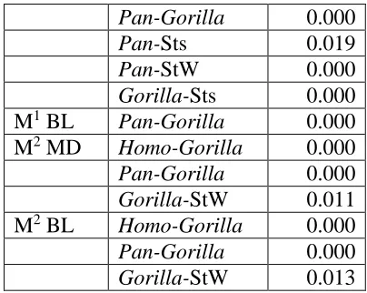
Table 7 exhibits the Tukey’s HSD significant differences (p < 0.05) for each unscaled tooth variable. Significantly distinct groups have a larger variation between than within the group. Homo is distinct from Gorilla and StW, Pan is distinct from Gorilla, and Gorilla differs significantly from all groups, for P3 MD. These significant differences are repeated for P3 BL, except that Pan is also distinct from StW. For P4 MD and BL, both Homo and Pan are distinct
from Gorilla, Sts and StW, and Gorilla differs significantly from Sts. An additional significant difference is for P4 MD where Gorilla is distinct from StW, and for P4 BL Sts differs from StW. For M1 MD, the extant species are all significantly different from one another, and Pan and
Gorilla are each distinct from Sts and StW. Homo and Pan are significantly different from
Gorilla, Sts and StW for M2 MD and BL, and for M3 MD. Gorilla is also significantly different
from Sts, for M2 BL. Finally, for M3 BL, Homo is distinct from Gorilla and StW, Pan is significantly different from Gorilla, Sts and StW, and Sts differs from StW.
Pan and Gorilla are distinct for every measurement, and Homo significantly differs from
Table 7 Tukey’s test results for each statistically significant species pairing by unscaled tooth variable.
Variable Relationship P value
P3 MD Homo-Gorilla 0.000
Homo-StW 0.018
Pan-Gorilla 0.000
Gorilla-Sts 0.008
Gorilla-StW 0.007
P3 BL Homo-Gorilla 0.000
Homo-StW 0.000
Pan-Gorilla 0.000
Pan-StW 0.001
Gorilla-Sts 0.000
Gorilla-StW 0.026
P4 MD Homo-Gorilla 0.000
Homo-Sts 0.002
Homo-StW 0.000
Pan-Gorilla 0.000
Pan-Sts 0.007
Pan-StW 0.013
Gorilla-Sts 0.007
Gorilla-StW 0.013
P4 BL Homo-Gorilla 0.000
Homo-Sts 0.004
Homo-StW 0.000
Pan-Gorilla 0.000
Pan-Sts 0.030
Pan-StW 0.000
Gorilla-Sts 0.030
Sts-StW 0.048
M1 MD Homo-Pan 0.003
Homo-Gorilla 0.000
Pan-Gorilla 0.000
Pan-Sts 0.001
Pan-StW 0.002
Gorilla-Sts 0.001
Gorilla-StW 0.031
M1 BL Homo-Gorilla 0.000
Homo-StW 0.006
Pan-Gorilla 0.000
Pan-StW 0.001
Gorilla-Sts 0.000
M2 MD Homo-Gorilla 0.000
Homo-Sts 0.003
Pan-Gorilla 0.000
Pan-Sts 0.001
Pan-StW 0.000
Gorilla-Sts 0.001
M2 BL Homo-Gorilla 0.000
Homo-Sts 0.004
Homo-StW 0.000
Pan-Gorilla 0.000
Pan-Sts 0.000
Pan-StW 0.000
M3 MD Homo-Gorilla 0.000
Homo-Sts 0.001
Homo-StW 0.000
Pan-Gorilla 0.000
Pan-Sts 0.001
Pan-StW 0.000
M3 BL Homo-Gorilla 0.000
Homo-StW 0.000
Pan-Gorilla 0.000
Pan-Sts 0.045
Pan-StW 0.000 Sts-StW 0.011
4.2.2 ANOVA and Tukey’s HSD Scaled
The ANOVA results show significant differences exist between the groups for each tooth variable (p < 0.009) for the scaled data, except for P4 MD (Table 8). For the scaled data, the F ratio has a wide range with the smallest at 1.248 for P4 MD and the largest at 132.849 for M1
MD. The F ratios show greater between group than within group variation as they are all greater than 1.0. The P value for the scaled data for P3 (MD and BL) are less than 0.05 indicating significance. The P value for P4 MD is 0.295 which means that this variable does not
Table 8 ANOVA for each scaled tooth variable.
Variable F ratio P value
P3 MD 3.635 0.008 P3 BL 3.565 0.009 P4 MD 1.248 0.295 P4 BL 7.342 0.000 M1 MD 132.849 0.000 M1 BL 5.800 0.000 M2 MD 22.537 0.000
M2 BL 22.075 0.000
The Tukey’s HSD significant differences (p < 0.05) for each scaled tooth variable are shown in Table 9. For P3 MD, Homo and Pan are significantly different from StW. Gorilla
differs from Sts, for P3 BL. All of the extant species are distinct from StW for P4 BL, and no species are significantly different for P4 MD. For M2 MD, Pan is distinct from all species, Homo
differs from all but Sts, and Gorilla is significantly different from all but StW. Pan and Gorilla
are the only species to be significantly different for M1 BL. For M2 MD and BL, Homo and Pan
are distinct from Gorilla, and Gorilla differs from StW.
For the premolars, P4 BL can distinguish the extant taxa from StW, and no species are significantly different for MD. For the molars, Homo, Pan and Gorilla are significantly different for every variable, meaning molar variables distinguish the extant species. StW is distinct from
Homo, Pan and Gorilla for three variables each.
Table 9 Tukey’s test results for each statistically significant species pairing by scaled tooth variable.
Variable Relationship P value
P3 MD Homo-StW 0.035
Pan-StW 0.024
P3 BL Gorilla-Sts 0.014
P4 BL Homo-StW 0.000
Pan-StW 0.000
Gorilla-StW 0.000
M1 MD Homo-Pan 0.019
Homo-Gorilla 0.000
Pan-Gorilla 0.000
Pan-Sts 0.019
Pan-StW 0.000
Gorilla-Sts 0.000
M1 BL Pan-Gorilla 0.000
M2 MD Homo-Gorilla 0.000
Pan-Gorilla 0.000
Gorilla-StW 0.011
M2 BL Homo-Gorilla 0.000
Pan-Gorilla 0.000
Gorilla-StW 0.013
4.3 Multivariate Analysis
4.3.1 Premolars Unscaled
The Jackknifed classification matrix for the unscaled premolars (Table 10) demonstrates that 76% of the specimens are classified correctly. The majority of Homo that are misclassified are classified as Pan. Pan only has 59% of the specimens classifying correctly and the majority that are not are classified as Homo. Homo, Pan and Gorilla all have one specimen that is classified as Sts. All of the StW specimens are in the correct category, as are 98% of the Gorilla
[image:50.612.70.272.70.231.2]specimens. None of the Sts specimens are in the correct category and 100% are misclassified as StW.
Table 10 Jackknifed classification matrix for the unscaled premolars.
Homo Pan Gorilla Sts StW %correct
Homo 23 8 0 1 0 72
Pan 14 22 0 1 0 59
Gorilla 0 0 39 1 0 98
Sts 0 0 0 0 2 0 StW 0 0 0 0 3 100 Total
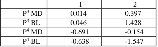
Figure 3 shows the relationship of the unscaled premolars for each specimen using the canonical discriminant function analysis. The variation explained by axis 1 is 94.5% and for axis 2 it is 5.5%. On axis 1, Homo and Pan are projected on the positive side, to a similar degree.
Gorilla is projected as a negative, as is StW. Sts is slightly negative, but as it is close to zero, it is difficult to classify. On axis 2, Homo, Pan and Gorilla are grouped together. Sts and StW are projected more negatively than the extant species. Table 11 supports Figure 3 with large negative loadings for the P4 variables on the first axis. On the second axis, Table 11 shows a large
[image:51.612.72.335.335.413.2]loading for BL values, for both P3 and P4. As the data are unscaled, this figure and table are size dependent.
Table 11 Canonical discriminant function for unscaled premolars.
1 2 P3 MD 0.014 0.397
P3 BL 0.046 1.428
P4 MD -0.691 -0.154
Figure 3 Scatterplot for unscaled premolars.
4.3.2 Molars Unscaled
Overall, 77% of the unscaled molar specimens are classified correctly using a Jackknifed classification (Table 12). Sixty nine percent of the Homo specimens classify as Homo, with the remainder classifying as either Pan or Sts. Pan classifies as Pan 78% of the time, with the majority of other specimens classified as Homo and one specimen as Sts. The majority of
Gorilla specimens classify correctly as Gorilla and 12% of the sample does not, and are
classified as Sts. Sts does not classify as Sts but as StW and Homo. Only half of StW classify as StW and the other half classify as Sts.
-10 -5 0 5
Table 12 Jackknifed classification matrix for unscaled molars.
Homo Pan Gorilla Sts StW %correct
Homo 22 7 0 3 0 69
Pan 7 29 0 1 0 78
Gorilla 0 0 35 5 0 88
Sts 1 0 0 0 1 0 StW 0 0 0 1 1 50 Total
30 36 35 10 2 77
The canonical discriminate function analysis of the unscaled molars for each species is shown in Figure 4. Variation explained by axis 1 is 93.6% variation and for axis 2 it is 6.4%. As the data are unscaled, this figure and table are size dependent. Homo and Pan are together on the negative side of axis 1, with Gorilla on the positive side. StW fossils are slightly positive and close to Gorilla. Sts are hard to classify as they are close to zero. All three extant species are similar on axis 2. With one exception (Sts 52), Sts and StW are negative on axis 2 due to distinct and large M2 BL variables. The sample size for Sts and StW was too small to create 68%
ellipses. Table 13 shows that M2 MD has a relatively large loading on axis 1. This table displays a large positive loading for M1 values and large negative M2 values for axis 2.
Table 13 Canonical discriminant function for unscaled molars.
1 2 M1 MD 0.357 1.052
M1 BL 0.296 0.799
[image:53.612.78.333.561.652.2]Figure 4 Scatterplot for unscaled molars.
4.3.3 Premolars Scaled
The Jackknifed classification matrix for the scaled premolars (Table 14) demonstrates a low degree of classification, 39% overall. Homo classifies as all other species, except Sts. The largest percentage is for StW, 67%, with one specimen being identified as Homo. Gorilla has the next highest correct classification rate at 48%. Gorilla and Pan each have a specimen which classifies as the other taxon. Sts classifies 100% as StW. In general, this classification matrix is greatly varied.
-5 0 5 10
Table 14 Jackknifed classification matrix for scaled premolars.
Homo Pan Gorilla Sts StW %correct
Homo 14 10 7 0 1 44
Pan 11 10 13 1 2 27
Gorilla 8 11 19 1 1 48
Sts 0 0 0 0 2 0 StW 1 0 0 0 2 67 Total
34 31 39 2 8 39
Figure 5 shows the relationship for scaled premolars for each species using the canonical discriminant function analysis, and 68% sample ellipses are displayed for all groups. The variation explained for axis 1 is 78.1% and for axis 2 it is 21.9%. As the data are scaled for size, the premolar variables are distinguished solely by shape. All of the extant species are clustered near zero on axes 1 and 2. For axis 2 Sts and StW are projected positively, with one outlier (Sts 24). For axis 2, the extant species molar dimensions are again distinct from the fossils, Sts and StW, and are located around zero. Table 15 shows high loadings for all P3 and P4 variables for
[image:55.612.74.316.562.647.2]axis 1. This is supported by the large overlap of extant species around zero. The P3 BL and P4 MD variables are positive on axis 2 as shown in Table 15.
Table 15 Canonical discriminant function for scaled premolars.
1 2 P3 MD 3.717 0.098
P3 BL 2.272 1.029 P4 MD 4.000 1.112
Figure 5 Scatterplot for scaled premolars.
4.3.4 Molars Scaled
Overall, 42% of the scaled molars classify correctly, according to the Jackknifed classification matrix (Table 16). Homo and Gorilla both are over 50% accurate. Homo, Pan, and Gorilla have specimens in every species category. Pan is only 8% accurate and the majority of specimens are classified as Homo and Sts. Sts and StW, both have 0% of the specimens classifying correctly, and both display as Homo and Pan, demonstrating poor classification.
-4 -3 -2 -1 0 1 2 3 4 5 6