Populating the mix space : parametric methods for generating multitrack audio mixtures

(1)

Po p ul a ti n g t h e m ix s p a c e :

p a r a m e t r i c m e t h o d s fo r

g e n e r a ti n g m u l ti t r a c k a u d i o

m ix t u r e s

Wilso n , AD a n d F a z e n d a , B M

h t t p :// dx. d oi.o r g / 1 0 . 3 3 9 0 / a p p 7 1 2 1 3 2 9

T i t l e

Po p ul a ti n g t h e m ix s p a c e : p a r a m e t r i c m e t h o d s fo r

g e n e r a ti n g m u l ti t r a c k a u d i o m ix t u r e s

A u t h o r s

Wils o n , AD a n d F a z e n d a , B M

Typ e

Ar ticl e

U RL

T hi s v e r si o n is a v ail a bl e a t :

h t t p :// u sir. s alfo r d . a c . u k /i d/ e p ri n t/ 4 4 6 1 3 /

P u b l i s h e d D a t e

2 0 1 7

U S IR is a d i gi t al c oll e c ti o n of t h e r e s e a r c h o u t p u t of t h e U n iv e r si ty of S alfo r d .

W h e r e c o p y ri g h t p e r m i t s , f ull t e x t m a t e r i al h el d i n t h e r e p o si t o r y is m a d e

f r e ely a v ail a bl e o nli n e a n d c a n b e r e a d , d o w nl o a d e d a n d c o pi e d fo r n o

n-c o m m e r n-ci al p r iv a t e s t u d y o r r e s e a r n-c h p u r p o s e s . Pl e a s e n-c h e n-c k t h e m a n u s n-c ri p t

fo r a n y f u r t h e r c o p y ri g h t r e s t r i c ti o n s .

(2)

Populating the Mix Space: Parametric Methods for

Generating Multitrack Audio Mixtures

Alex Wilson * and Bruno M. Fazenda

Acoustics Research Centre, School of Computing, Science and Engineering, University of Salford, Greater Manchester, Salford M5 4WT, UK; [email protected]

* Correspondence: [email protected] Academic Editor: Tapio Lokki

Received: 31 October 2017; Accepted: 4 December 2017; Published: 20 December 2017

Featured Application: The numerical methods described in this paper can be used in the automatic creation of artificial datasets of audio mixes, as real-world mixes are both scarce and costly to produce. Such datasets can be used for a variety of applications, such as material for signal analysis, audio stimuli in psychoacoustic testing or as a population of solutions to be optimised, thus forming the basis of an automatic mixing system. Within this paper, the application of interest is testing the robustness of tempo estimation to re-mixing.

Abstract: The creation of multitrack mixes by audio engineers is a time-consuming activity and creating high-quality mixes requires a great deal of knowledge and experience. Previous studies on the perception of music mixes have been limited by the relatively small number of human-made mixes analysed. This paper describes a novel “mix-space”, a parameter space which contains all possible mixes using a finite set of tools, as well as methods for the parametric generation of artificial mixes in this space. Mixes that use track gain, panning and equalisation are considered. This allows statistical methods to be used in the study of music mixing practice, such as Monte Carlo simulations or population-based optimisation methods. Two applications are described: an investigation into the robustness and accuracy of tempo-estimation algorithms and an experiment to estimate distributions of spectral centroid values within sets of mixes. The potential for further work is also described.

Keywords:intelligent music production; music information retrieval; multitrack mixing; stereo panning; audio equalisation; tempo estimation; spectral centroid

1. Introduction

The mixing of audio signals is a complicated optimisation problem, in which an audio engineer must consider a vast number of technical and aesthetic considerations in order to achieve the desired result. Traditionally, many tasks in audio mixing are performed on a mixing console. Typically, such a device consists of a series of channel strips, one representing each audio track, on which various operations can be performed such as adjustments in equalisation, panning and overall level. While this format is useful for allowing a hands-on interaction with the audio content, it is not the most direct or efficient way of exploring these parameters and discovering mixes in the process.

One legacy of this console design philosophy is that, in the literature, it has become commonplace to define a mix as the sum of the input tracks, subject to control vectors for gain, panning, equalisation etc., [1–3]. Subsequently, a number of publications [4–6] have referred to a mix ofntracks as a point in ann-dimensional vector space, with each axis as the gain of a given track. While effective in certain cases, and certainly straightforward to visualise, this definition produces a solution space which is sub-optimal when searching for mixes.

(3)

Appl. Sci. 2017,7, 1329 2 of 21

The following are equations used to define a mix, according to various previous works. Note that the nomenclature has not been changed from the original texts. Equation (1) was used by [1], stating simply that a mix is the sum of all individual channels.

mix=

N

∑

n=1

Chn[t] (1)

This definition seems logical and even trivial, if inspired by a summing mixer, and has become the foundation for a series of more elaborate definitions, such as adding a gain vector,ato each track, allowing for time-dependent changes to the track gains, simulating the movement of individual faders [2].

y[n] =

K

∑

k=1

ak[n]×xk[n] (2)

In a review paper from 2011 [3], Equation (3) was used, adding generic control vectorscwhich modulate the input signalsx. These control vectors allow for a variety of results, such as polarity correction, delay correction, panning and source separation, depending on their implementation.

mixl(n) = M−1

∑

m=0

K−1

∑

k=0

ck,m,l(n)×xm(n) (3) Each of these equations considers the mix as the sum of the input tracks, although there is little agreement on terminology or nomenclature in this general definition. What is important to realise here is that these expressions characterise not strictly the mix itself but the output of a summing mixer, or conventional fader-based mixing console. As will be shown in Section2, the set of unique mixes is a subset of this set, as illustrated by Equation (4). We refer to this subset as the mix-space, introduced in [7]. It is this space that a mixing console should directly explore, rather than the gain-space. Section2 presents an updated definition of the termmix, which produces concise solution spaces by exploring only the parameter space φ, avoiding the redundancies in g, which represents the gain vector of

the system.

g1,g2,g3, . . . ,gn

| {z }

gain-space

= r

|{z}

master volume

,φ1,φ2, . . . ,φn−1

| {z }

mix-space

(4)

The primary contributions of this work are as follows: (a) the mix-space as a theoretical framework in which existing audio mixes can be examined, in contrast to the gain-space, and (b) methods for the generation of audio mixes in the mix-space. These contributions are described in Section2.

The creation of artificial datasets relating to music mixing practice helps to overcome one of the main obstacles in the field of mix analysis, which is the lack of available data and the cost associated with gathering new data from mix engineers. Thus far, it has been difficult to make statistical inference about music mixing practice as available studies have only had access to small datasets of user-generated audio mixes, with few exceptions [8].

Thus far, the numerical methods in this paper have been applied in creating an initial population for evolutionary algorithms [9,10]. Further applications are explored in Section3 and discussed in Section4.

2. Theoretical Framework

(4)

2.1. Track Gains

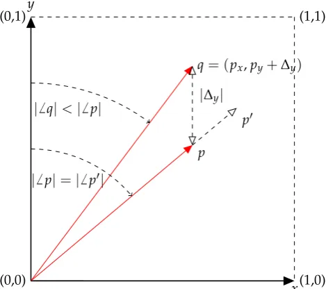
Consider the trivial case where two audio signals are to be mixed, where only the absolute levels of each signal can be adjusted. In Figure1, the gains of two signals are represented byxandy, where both are positive-bound. Consider the pointpas a configuration of the signal gains, i.e.,(px,py). From this point, the values ofxandyare both increased in equal proportion, arriving at the pointp0_. The magnitude ofpis less than that ofp0₍_k_p_k_<_k_p0_k_{) yet since the ratio of}_x_to_y_{is identical, the angles} subtended by the vectors from they-axis are equal (6 _p₌6 _p0_{). In the context of a mix of two tracks,} what this means is that the volume ofp0_{is greater than}_p_{, yet the blend of input tracks is the same.}

2.1. Track Gains

Consider the trivial case where two audio signals are to be mixed, where only the absolute levels of each signal can be adjusted. In Figure1, the gains of two signals are represented byxandy, where both are positive-bound. Consider the pointpas a configuration of the signal gains, i.e.,(px,py). From this point, the values ofxandyare both increased in equal proportion, arriving at the pointp0_. The magnitude ofpis less than that ofp0₍_k_p_k_<_k_p0_k_{) yet since the ratio of}_x_to_y_{is identical, the angles} subtended by the vectors from they-axis are equal (6 _p=6 _p0_{). In the context of a mix of two tracks,} what this means is that the volume ofp0_{is greater than}_p_{, yet the blend of input tracks is the same.}

(0,0) (0,1)

(1,0) (1,1)

x y

p

p0

|∆y|

q= (px,py+∆y)

|6 _q_|_<_|6 _p_|

[image:4.595.181.421.215.423.2]

|6 _p_|₌_|6 _p0_|

Figure 1.Pointsp,p0_and_r_{, in 2-track gain space. Note that the audio output at points}_p_and_p0_{is the}

same ‘mix’.

As an alternate to Equation (1), a mix can be thought of as the relative balance of audio signals. From this definition, the pointsp andp0 _{are the same mix, only}_p0 _{is being presented at a greater} volume. If the listener has control over the master volume of the system, then any difference between

pandp0_{becomes ambiguous.}

Definition 1. Mix: an audio stream constructed by the superposition of others in accordance with a specific blend, balance or ratio.

From p, the level of fadery can be increased by∆y, arriving atq. In this particular example, the value of ∆y was chosen such that kqk = kp0k. However, for any |∆y| > 0, 6 q 6= 6 p0. Therefore,qclearly represents a different mix to eitherporp0_{. Consequently, the definition of a mix is} clarified by what it is not: when two audio streams contain the same blend of input tracks but the result is at different overall amplitude levels, these two outputs can be considered the same mix. For this mixing example, where there aren=2 signals, represented byngain values, the mix is dependant on

n−1 variables; in this case, the angle to the vector. The`2norm of the vector is simply proportional to the overall loudness of the mix.

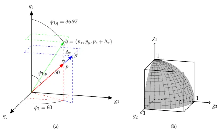
Figure2a shows a similar structure, withn = 3. Here, the point p0 _{is also an extension of} _p_. As in Figure1,qis located by increasing the value ofyfrom the pointpandkqk=kp0_k_{. Here, the values} of each angle are explicitly determined and displayed. All three vectors share the equatorial angle of 60◦_{. The polar angle of}_p_and_p0_{is 50}◦_{, while the polar angle of}_q_{is less than this, at}_≈₃₇◦_{. As in the} two-dimensional case, it is the angles which determine the parameters of the mix and the norm of the vector is related to the overall loudness.

Figure 1.Pointsp,p0_and_r_{, in 2-track gain space. Note that the audio output at points}_p_and_p0_{is the}

same ‘mix’.

As an alternate to Equation (1), a mix can be thought of as the relative balance of audio signals. From this definition, the pointsp andp0 _{are the same mix, only}_p0 _{is being presented at a greater} volume. If the listener has control over the master volume of the system, then any difference between

pandp0_{becomes ambiguous.}

Definition 1. Mix: an audio stream constructed by the superposition of others in accordance with a specific blend, balance or ratio.

From p, the level of fadery can be increased by∆y, arriving atq. In this particular example, the value of ∆y was chosen such that kqk = kp0k. However, for any |∆y| > 0, 6 q 6= 6 p0. Therefore,qclearly represents a different mix to eitherporp0_{. Consequently, the definition of a mix is} clarified by what it is not: when two audio streams contain the same blend of input tracks but the result is at different overall amplitude levels, these two outputs can be considered the same mix. For this mixing example, where there aren=2 signals, represented byngain values, the mix is dependant on

n−1 variables; in this case, the angle to the vector. The`2norm of the vector is simply proportional to the overall loudness of the mix.

(5)

[image:5.595.122.474.81.290.2]

Appl. Sci. 2017,7, 1329 4 of 21

Figure 2.Graphical representation of three mixes in mix-space. While shown for three tracks, this is generalisable to any number of tracksn, using hyperspherical coordinates. (a) Mix at a point in 3-track gain space. Note that the audio output at pointspandp0_{is the same ‘mix’, despite the vectors having}

different lengths in this space; (b) For a 3-track mixture, while the cube (R3_{) represents all outputs of}

a summing mixer, the surface of the sphere (S2_{) represents all possible mixes.}

While Figures1and2a show a space of track gains, there is clearly a redundancy of mixes in this space. What is ultimately desired is a space of mixes.

Definition 2. Mix-space: a parameter space containing all the possible audio mixes that can be achieved using a defined set of processes.

It becomes apparent that a Euclidean space with track gains as basis vectors is not an efficient way to represent a space of mixes, according to Definition2. This explains why Equation (1) would not be appropriate when searching for mixes. If, in Figure2a, a set ofmpoints randomly selected on

R3_{were chosen, the number of mixes could be less than}_m_{, as the same mix could be chosen multiple} times at different overall volumes. A set ofmrandomly selected points on a sphere of any radius (S2₎ would result in a number of mixes equal tom. This surface is represented in Figure2b, which shows the portion of a unit-sphere in positively-unbounded_R3_{, upon which exist all possible mixes of three tracks.}

While both the 2-content of_S2_{(surface area) and the 3-content of the enclosing}_R3_{, (volume) both,} strictly, contain an infinite amount of points, the reduced dimensionality ofS2_{makes it a more attractive} content to use in optimisation, as_S2_{is a subset of}_R3_{(in this context,}_content_{can be considered as} “hypervolume”. Seehttp://mathworld.wolfram.com/Content.html). As a consequence, themix-space,

φ, is a more compact representation of audio mixes than the gain-space,g.

(6)

Appl. Sci. 2017,7, 1329 5 of 21

r= pgn2+gn−12+· · ·+g22+g12

φi= arccos√_g gi

n2+gn−12+···+gi2 , wherei= [1, 2, . . . ,n−3],i∈Z

...

φn−2= arccos√_g2_n+_ggn−2

n−12+gn−22

φ_n₋1=

    

arccos_√ gn−1

g2_n₊_g_n

−12 gn ≥0

2π−arccos_√ gn−1

g2_n₊_g_n

−12 gn <0

(5)

g1= rcosφ1

gj= rcosφj∏ij−1=1sinφi, wherej= [2, 3, . . .n−2],j∈Z gn= r∏n_i₌−₁1sinφi

(6)

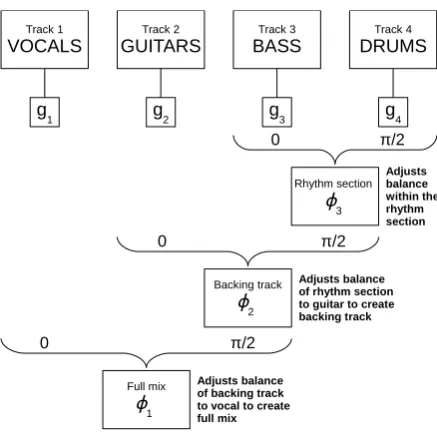
Figure3represents a comparable 4-track mixing exercise, as described in [7]. The four audio sources were specifically chosen for this example (vocals, guitar, bass and drums) and assigned to

g1,g2,g3andg4respectively. Consequently, the set of mixes is represented by a 3-sphere of radiusr. Due to the deliberate assignment of tracks in this example, the parametersφ1,φ2andφ3represent a set of inter-channel balances which, due to the specific relationships of instruments, have importance to musicians and audio engineers:φ3determines the balance of bass to drums, the rhythm section in this case;φ2describes the projection of this balance onto theg2axis, i.e., the blend of guitar to rhythm section, and finally,φ₁describes the balance of the vocal to this backing track.

r=qgn2+gn−12+· · ·+g22+g12 (5a)

φi=arccosp gi

gn2+gn−12+· · ·+gi2

, wherei= [1, 2, . . . ,n−3],i∈Z (5b) ...

φn−2=arccosp gn−2 g2

n+gn−12+gn−22

(5c)

φn−1=

    

arccos_√ gn−1

g2

n+gn−12 gn ≥0

2π−arccos_√ gn−1

g2_n₊_g_n

−12 gn <0

(5d)

g1=rcosφ1 (6a)

gj=rcosφj j−1

∏

i=1

sinφ_i, wherej= [2, 3, . . .n−2],j∈Z (6b)

gn=r n−1

∏

i=1

sinφi (6c)

Figure3represents a comparable 4-track mixing exercise, as described in [7]. The four audio sources were specifically chosen for this example (vocals, guitar, bass and drums) and assigned to

g1,g2,g3andg4respectively. Consequently, the set of mixes is represented by a 3-sphere of radiusr. Due to the deliberate assignment of tracks in this example, the parametersφ1,φ2andφ3represent a set of inter-channel balances which, due to the specific relationships of instruments, have importance to musicians and audio engineers:φ3determines the balance of bass to drums, the rhythm section in this case;φ2describes the projection of this balance onto theg2axis, i.e., the blend of guitar to rhythm section, and finally,φ1describes the balance of the vocal to this backing track.

Track 1

VOCALS GUITARSTrack 2 BASSTrack 3 DRUMSTrack 4

Rhythm section φ₃ Backing track φ₂ Full mix φ₁ Adjusts balance within the rhythm section Adjusts balance of rhythm section to guitar to create backing track

Adjusts balance of backing track to vocal to create full mix

g₁ g₂ g₃ g₄

0 π/2

[image:6.595.188.407.383.602.2]

0 π/2

Figure 3.Schematic representation of a four-track mixing task, with track gainsg1,g2,g3,g4, and the

semantic description of the threeφterms, when adjusted from 0 toπ/2. Figure taken from [7].

Figure 3.Schematic representation of a four-track mixing task, with track gainsg1,g2,g3,g4, and the

semantic description of the threeφterms, when adjusted from 0 toπ/2. Figure taken from [7].

From here, the parameter space comprising then−1 angular components of the hyperspherical coordinates of a (n−1)-sphere in an-dimensional gain-space, is referred to as a (n−1)-dimensional mix-space. More simply, this can be stated by saying the mix-space is the surface of a hypersphere in gain-space. In the case of music mixing, only the positive values ofgare of interest. Subsequently, the interesting region of the mix-space is only a small proportion of the total hypersurface. This fraction is 1/2n_.

As each point in φ represents a unique mix, the process of mixing can be represented as

(7)

Appl. Sci. 2017,7, 1329 6 of 21

walk is a simple Brownian motion (http://people.sc.fsu.edu/~jburkardt/m_src/brownian_motion_ simulation/brownian_motion_simulation.html). After 30 s, the walk is stopped and the final point reached is marked ‘×’. The gain values for each of the three tracks are shown in Figure4b and it is clear that the random walk is on a 2-sphere, as anticipated. The time-series of gain values is shown in Figure4c. Note thatg∈[−1, 1], so for positivegthe region explored is as represented in Figure2b.

Appl. Sci. 2017,7, x 6 of 23

walk is a simple Brownian motion (http://people.sc.fsu.edu/~jburkardt/m_src/brownian_motion_

simulation/brownian_motion_simulation.html). After 30 s, the walk is stopped and the final point reached is marked ‘

×

’. The gain values for each of the three tracks are shown in Figure4b and it is clear that the random walk is on a 2-sphere, as anticipated. The time-series of gain values is shown in Figure4c. Note thatg

∈

[

₋

1, 1

]

, so for positivegthe region explored is as represented in Figure2b.

−4 −2 0

φ1

φ2

(a)

−1 0

1

−1 0 1 −1 0 1

g₃ g₂

g1

(b)

0 2 4 6 8 10 12 14 16 18 20 22 24 26 28 30

−1 −0.5 0 0.5 1

Time (s)

Gain

(linear)

g₁ g₂ g₃

(c)

Figure 4.A time-varying mix can be considered as a path in the mix-space. Here, a random time-varying mix is generated by means of a random walk. (a) Random walk in mix-space; Brownian motion, halted after 30 s; (b) Random walk from Figure4a converted to gain-space; (c) Time series of gain values for each of the three tracks.

When presented in isolation, such a random mix, whether static or time-varying, may be unrealistic. It is hypothesised that real mix engineers do not carry out a random walk but a guided and informed walk, from some starting point (“source”) to their ideal final mix (“sink”). For further discussion of these terms, see [7], which uses the mix-space as a framework for the analysis of a simple 4-track mixing experiment. The power in these methods comes from generating a large number of mixes, more so than realistically could be obtained from real-world examples, and estimating parameters using statistical methods. Further generation and statistical analysis of time-varying mixes is left to further work.

Figure 4.A time-varying mix can be considered as a path in the mix-space. Here, a random time-varying mix is generated by means of a random walk. (a) Random walk in mix-space; Brownian motion, halted after 30 s; (b) Random walk from Figure4a converted to gain-space; (c) Time series of gain values for each of the three tracks.

When presented in isolation, such a random mix, whether static or time-varying, may be unrealistic. It is hypothesised that real mix engineers do not carry out a random walk but a guided and informed walk, from some starting point (“source”) to their ideal final mix (“sink”). For further discussion of these terms, see [7], which uses the mix-space as a framework for the analysis of a simple 4-track mixing experiment. The power in these methods comes from generating a large number of mixes, more so than realistically could be obtained from real-world examples, and estimating parameters using statistical methods. Further generation and statistical analysis of time-varying mixes is left to further work.

2.2. Generating Gain Vectors by Sampling the Mix-Space

(8)

Appl. Sci. 2017,7, 1329 7 of 21

(n−1)-sphere, points are generated from a von-Mises–Fisher (vMF) distribution. The probability density function of the vMF distribution for a randomn-dimensional unit vectorxis given by

fn(x;µ,κ) =Cn(κ)eκµTx

whereκ≥0,||µ||=1,n≥2 and the normalisation constantCn(κ)is given by Cn(κ) = κ

n/2−1

(2π)n/2In/2−1(κ).

Here,Ivis the modified Bessel function of the first kind at orderv. The parametersµandκare called the mean direction and concentration parameter, respectively. The greater the value ofκ,

the higher the concentration of the distribution around the mean direction µ, resulting in lower

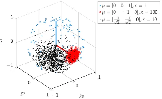
variance. The distribution is unimodal forκ >0 and is uniform on_Sn−1_for_κ ₌_{0. Further details} can be found in [12,13]. TheSphericalDistributionsRand(https://github.com/yuhuichen1015/ SphericalDistributionsRand) code, based on the work of [14], was used to generate points according to a vMF distribution. In the context of audio mixes,µ(where|µ|=1) represents the mix about which others are distributed, akin to the mean in a normal distribution. Theκterm represents the diversity of

mixes generated, analogous (but inversely proportional) to variance. An example is shown in Figure5, where three distributions are drawn from a 2-sphere.

2.2. Generating Gain Vectors by Sampling the Mix-Space

A set of mixes can be generated by choosing points in the mix-space. In selecting a suitable parametric distribution, it is important to note that linear distributions, such as the normal distribution, are not appropriate as the domain in question is not linear but a spherical surface. The statistics of such distributions are described by a number of equivalent terms in the literature, such as circular, spherical or directional statistics. In order to generate points close to a desired position on the

(n−1)-sphere, points are generated from a von-Mises–Fisher (vMF) distribution. The probability

density function of the vMF distribution for a randomn-dimensional unit vectorxis given by

fn(x;µ,κ) =Cn(κ)eκµTx

whereκ≥0,||µ||=1,n≥2 and the normalisation constantCn(κ)is given by

Cn(κ) = κ n/2−1

(2π)n/2In/2−1(κ).

Here,Ivis the modified Bessel function of the first kind at orderv. The parametersµandκare

called the mean direction and concentration parameter, respectively. The greater the value of κ,

the higher the concentration of the distribution around the mean direction µ, resulting in lower

variance. The distribution is unimodal forκ > 0 and is uniform onSn−1_for_κ ₌ _{0. Further details} can be found in [12,13]. TheSphericalDistributionsRand(https://github.com/yuhuichen1015/ SphericalDistributionsRand) code, based on the work of [14], was used to generate points according to a vMF distribution. In the context of audio mixes,µ(where|µ|=1) represents the mix about which

others are distributed, akin to the mean in a normal distribution. Theκterm represents the diversity of

mixes generated, analogous (but inversely proportional) to variance. An example is shown in Figure5, where three distributions are drawn from a 2-sphere.

−1 0

1

−1 0 1 −1 0 1

g3

g2

g1

µ= [0 0 1],κ=1 µ= [0 −1 0],κ=100 µ= [−√1

[image:8.595.172.432.363.522.2]

2 −√12 0],κ=10

Figure 5. Three sets of mixes, drawn from the mix-space. This shows the effect of varying the concentration parameterκ, that a larger value results in less diversity.

2.2.1. Simple Mixing Model

From here, the example mixing session described is an 8-track session, containing vocals, guitars, bass and drums [15]. Forn=8 tracks, the gains required for the equal-loudness mix (once all audio tracks have been normalised in perceived loudness) are distributed around the followingµ—each

track gain is equal ton−2_{, such that}_|_µ_|₌_1.

µ= [0.3536 0.3536 0.3536 0.3536 0.3536 0.3536 0.3536 0.3536]

Figure 5. Three sets of mixes, drawn from the mix-space. This shows the effect of varying the concentration parameterκ, that a larger value results in less diversity.

2.2.1. Simple Mixing Model

From here, the example mixing session described is an 8-track session, containing vocals, guitars, bass and drums [15]. Forn=8 tracks, the gains required for the equal-loudness mix (once all audio

tracks have been normalised in perceived loudness) are distributed around the followingµ—each

track gain is equal ton−2_{, such that}_|_µ_|₌_1.

µ= [0.3536 0.3536 0.3536 0.3536 0.3536 0.3536 0.3536 0.3536]

Previous studies have indicated that, while a good initial guess, presenting each track at equal loudness is not an ideal final mix. As suggested by three recent PhD theses on the topic [15–17], vocals are often the loudest element in a mix. To this equal loudness configuration, a vocal boost is added according to p.157 of [16], i.e., a boost of 6.54 dB. This addition of 6.54 dB to the vocal track produces the following vector, where track 8 is vocals.

(9)

Appl. Sci. 2017,7, 1329 8 of 21

If the previous vector was, then it is clear that this point is no longer on the unit 7-sphere. To project the point back onto the unit 7-sphere, the vector is normalised by dividing by the`2(Euclidean) norm, resulting in the following.

µ= [0.2948 0.2948 0.2948 0.2948 0.2948 0.2948 0.2948 0.6259] (7)

This vector is the newµon the unit 7-sphere about which a set of mixes will be generated.

The result is shown in Figure6a. Each mix generated draws a gain value for each track such that the

`2norm is equal to 1. Note that the median values closely match the vectorµ, as expected. Of course, there may not exist a mix which has these median values. This specific value ofκwas chosen to avoid

generating negative gains, achieved through trial and error. For a distribution which produces negative gains, the absolute value could be taken to avoid inverting the phase of the tracks. Ignoring phase, a gain ofgis perceptually equal to−g, meaning that the shape of the distribution would be altered if negative gains were included.

Appl. Sci. 2017,7, x 8 of 23

Previous studies have indicated that, while a good initial guess, presenting each track at equal loudness is not an ideal final mix. As suggested by three recent PhD theses on the topic [15–17], vocals are often the loudest element in a mix. To this equal loudness configuration, a vocal boost is added according to p.157 of [16], i.e., a boost of 6.54 dB. This addition of 6.54 dB to the vocal track produces the following vector, where track 8 is vocals.

µ= [0.3536 0.3536 0.3536 0.3536 0.3536 0.3536 0.3536 0.7507]

If the previous vector was, then it is clear that this point is no longer on the unit 7-sphere. To project the point back onto the unit 7-sphere, the vector is normalised by dividing by the`2(Euclidean) norm,

resulting in the following.

µ= [0.2948 0.2948 0.2948 0.2948 0.2948 0.2948 0.2948 0.6259] (7)

This vector is the new µon the unit 7-sphere about which a set of mixes will be generated.

The result is shown in Figure6a. Each mix generated draws a gain value for each track such that the

`2norm is equal to 1. Note that the median values closely match the vectorµ, as expected. Of course,

there may not exist a mix which has these median values. This specific value ofκwas chosen to avoid

generating negative gains, achieved through trial and error. For a distribution which produces negative gains, the absolute value could be taken to avoid inverting the phase of the tracks. Ignoring phase, a gain ofgis perceptually equal to−g, meaning that the shape of the distribution would be altered if negative gains were included.

OH1OH2Kick Snr BassGtr1Gtr2 Vox 0

0.2 0.4 0.6 0.8

Gain

(a)

OH1OH2Kick Snr BassGtr1Gtr2 Vox 0

0.2 0.4 0.6 0.8

[image:9.595.122.480.289.411.2]

(b)

Figure 6.Boxplots of track gains for two generated datasets of mixes, drawn from separate distributions. (a)µ=Equation (7),κ=200; (b)µ=Equation (8),κ=200

2.2.2. Perceptual Mixing Model

Rather than a simple vocal boost, what is required is a more informed choice of instrument levels. In [7], a simple 4-track mixing exercise was reported, where participants created mixes of vocals, guitars, bass and drums using only volume faders. This experiment was expanded to an 8-track format, as in this paper, and is reported in [15]. Participants were asked the same task, only this time stereo-panning and a basic 3-band EQ was added. The median instrument levels obtained from this experiment are shown in Equation (8). Since participants had the ability to pan sources; the median levels were available for left and right channels separately, which are shown in Equations (10) and (11). Figure6b shows the mixes obtained when the target vector is based on these median track levels, known asµinformed. It can be seen that the levels of bass guitar and kick drum are higher than average,

while drum overheads have been attenuated. Vocals are set high in the mix, as seen in the mono experiment [7,15] and other previous studies [16,17]. Matlab code for generating sets of mixes, as in Figure6, is available for download (https://github.com/alexwilson101/PopulateMixSpace).

µinformed = [0.2254 0.2282 0.3221 0.2679 0.4437 0.3616 0.3221 0.5387] (8)

Figure 6.Boxplots of track gains for two generated datasets of mixes, drawn from separate distributions. (a)µ=Equation (7),κ=200; (b)µ=Equation (8),κ=200

2.2.2. Perceptual Mixing Model

Rather than a simple vocal boost, what is required is a more informed choice of instrument levels. In [7], a simple 4-track mixing exercise was reported, where participants created mixes of vocals, guitars, bass and drums using only volume faders. This experiment was expanded to an 8-track format, as in this paper, and is reported in [15]. Participants were asked the same task, only this time stereo-panning and a basic 3-band EQ was added. The median instrument levels obtained from this experiment are shown in Equation (8). Since participants had the ability to pan sources; the median levels were available for left and right channels separately, which are shown in Equations (10) and (11). Figure6b shows the mixes obtained when the target vector is based on these median track levels, known asµinformed. It can be seen that the levels of bass guitar and kick drum are higher than average, while drum overheads have been attenuated. Vocals are set high in the mix, as seen in the mono experiment [7,15] and other previous studies [16,17]. Matlab code for generating sets of mixes, as in Figure6, is available for download (https://github.com/alexwilson101/PopulateMixSpace).

µ_informed= [0.2254 0.2282 0.3221 0.2679 0.4437 0.3616 0.3221 0.5387] (8)

2.3. Track Panning

Thus far, only mono mixes have been considered, where all audio tracks are summed to one channel. In creative music production, it is rare that mono mixes are encountered. The same mathematical formulations of the mix-space can be used to represent panning. Consider Figure4, which shows track gains in the range[−1, 1]. Should these be replaced with track pan positions

(10)

mix-space (or “pan-space”) can be used to generate a position for each track in the stereo field. To avoid confusion with the earlier use ofφ, the pan-space is denoted byθ, although the formalism

is identical.

p1,p2,p3, . . . ,pn

| {z }

absolute panning

=rpan

|{z}

width-scaling

,θ1,θ2, . . . ,θn−1

| {z }

pan-space

(9)

However, the mix-space for gains (φ) takes advantage of the fact that a mix (in terms of track

gains only) is comprised of a series of inter-channel gain ratios, meaning that the radiusris arbitrary and represents a master volume. In terms of track panning, one obtains a series of inter-channel panning ratios, the precise meaning of which is not intuitive. Additionally, the radiusrpanwould still be required to determine the exact pan position of the individual tracks. Therefore, the pan-space describes the relative pan positions of audio tracks to one another.

For a simple example with only two tracks, the meaning ofrpan andθis relatively simple to understand. Consider the unit circle in a plane where the Cartesian coordinates(x,y)represent the pan positions of two tracks, as shown in Figure7. MixAis at the point(√1

2,√12): both tracks are panned at the same position. As this is a circle with arbitrary radius,rpan, then the radius controls how far positive (right) the two tracks are panned, from 0 (centre) to+1 (far right). MixBdoes the same

but towards the left channel. One may ask whetherAandBare identical “panning-mixes”, aspand

p0_{in Figure}₁_{were identical “level-mixes”?}

[image:10.595.208.391.455.634.2]

Now consider mixC, where one track is panned left and the other right. MixDis simply the mirror image of this. Aretheseto be considered as the same mix, or as different mixes? Here,rpan adjusts the distance between the two tracks, from both centre whenrpan = 0, to(−1, 1)whenrpan = √2 (as indicated by mixC0_{). Does a change in}_r_pan _{change the mix, or is it simply the same mix only} wider/narrower? Overall, the angleθadjusts the panning mix andrpanis used to obtain absolute positions in the stereo field, at a particular width-scale (i.e., to zoom in or zoom out).

Figure 7.Panning of two tracks, represented as a 1-sphere. The panning mix is determined by the angleθwithrpanacting as a scaling variable, adjusting the overall width of the mix. For example,C0is

a wider version ofC.

2.3.1. Method 1—Separate Left and Right Gain Vectors

(11)

Appl. Sci. 2017,7, 1329 10 of 21

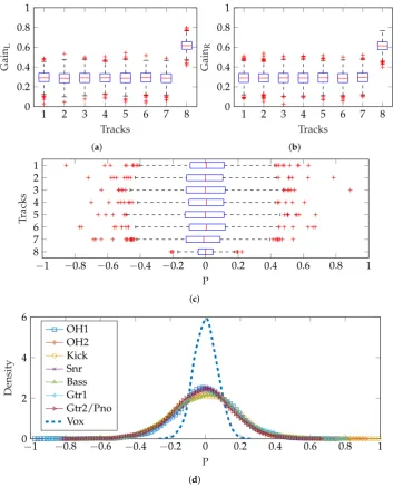
zero, the panning of the vocals is much less wide than the other tracks. Additionally, sinceκ =200 was chosen to prevent any negative gains, there are few zero-gain instances; therefore, there is a lack of hard-panning. Figure8a,b show the gain settings produced and a boxplot of the resulting pan positions is shown in Figure8c, where the inter-quartile range extends to±0.4 for the seven instrument tracks and about±0.2 for the vocals. The estimated density of pan positions for each track is shown, illustrating the relatively narrow vocal panning. As expected, these estimated density functions are Gaussian, to a good approximation.

Appl. Sci. 2017,7, x 11 of 24

1 2 3 4 5 6 7 8

0 0.2 0.4 0.6 0.8 1

Tracks

Gain

L

(a)

1 2 3 4 5 6 7 8

0 0.2 0.4 0.6 0.8 1

Tracks

Gain

R

(b)

−1 −0.8 −0.6 −0.4 −0.2 0 0.2 0.4 0.6 0.8 1 1

2 3 4 5 6 7 8

P

Tracks

(c)

−1 −0.8 −0.6 −0.4 −0.2 0 0.2 0.4 0.6 0.8 1 0

2 4 6

P

Density

OH1 OH2 Kick Snr Bass Gtr1 Gtr2/Pno Vox

[image:11.595.119.474.198.636.2]

(d)

Figure 8.Panning method 1—separate vMF distributions for gain_Land gain_R, both using Equation (7). (a) Boxplot of track gains for left channel, using Equation (7); (b) Boxplot of track gains for right channel, using Equation (7); (c) Boxplot of pan positions for each track; (d) Probability density of pan positions for each track.

Rather than using the sameµfor both left and right channels, a unique choice ofµLandµRcan

be made, as described in Section2.2.2. The vectors used are shown in Equations (10) and (11). When summed to mono, this is equivalent to Equation (8).

µL= [0.2741 0.1354 0.3361 0.2657 0.4401 0.3796 0.2566 0.5651] (10)

µR= [0.1189 0.2597 0.3162 0.2612 0.4683 0.2935 0.3727 0.5531] (11)

Figure9shows the difference in gains produced for left and right channels. There were some negative track gains produced: when generating audio mixes, the absolute magnitude of the gain was used to avoid phase inversions which would alter spatial perception of the stereo overhead pair. It is Figure 8.Panning method 1—separate vMF distributions for gain_Land gain_R, both using Equation (7). (a) Boxplot of track gains for left channel, using Equation (7); (b) Boxplot of track gains for right channel, using Equation (7); (c) Boxplot of pan positions for each track; (d) Probability density of pan positions for each track.

(12)

µL= [0.2741 0.1354 0.3361 0.2657 0.4401 0.3796 0.2566 0.5651] (10)

µR= [0.1189 0.2597 0.3162 0.2612 0.4683 0.2935 0.3727 0.5531] (11)

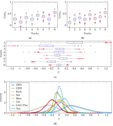
Figure9shows the difference in gains produced for left and right channels. There were some negative track gains produced: when generating audio mixes, the absolute magnitude of the gain was used to avoid phase inversions which would alter spatial perception of the stereo overhead pair. It is clear that the similarity of vocals gains in left and right channels produces a limited variety of pan positions close to the central position, as shown in Figure9c,d. Other instruments are panned with mean position and variance in accordance with the experimental results [15].

Appl. Sci. 2017,7, x 12 of 24

1 2 3 4 5 6 7 8

0 0.5 1

Tracks

Gain

L

(a)

1 2 3 4 5 6 7 8

0 0.5 1

Tracks

Gain

R

(b)

−1.2 −1 −0.8 −0.6 ₋0.4 −0.2 0 0.2 0.4 0.6 0.8 1 1.2 1

2 3 4 5 6 7 8

P

Tracks

(c)

−1.2 −1 −0.8 −0.6 ₋0.4 −0.2 0 0.2 0.4 0.6 0.8 1 1.2 0

2 4 6

P

Density

OH1 OH2 Kick Snr Bass Gtr Gtr2/Pno Vox

[image:12.595.110.486.238.655.2]

(d)

Figure 9.Panning method 1b—separate vMF distributions for left and right channels but using unique µvectors, shown in Equations (10) and (11). (a) Boxplot of track gains for left channel, using Equation (10); (b) Boxplot of track gains for right channel, using Equation (11); (c) Boxplot of pan positions for each track. Where|P|>1, this is caused by negative track gains; (d) Probability density of pan positions for each track.

2.3.2. Method 2—Separate Gain and Panning

This method involved generating random mono mixes as Section2.2(using Equation (7) and then generating pan positions separately. Aµpanwas created for a vMF distribution. This vector was based

on experimental results reported in [15], which showed that, generally, overheads and guitars were widely panned while kick, snare, bass and vocals were positioned centrally.

µpan= [−0.5 0.5 0 0 0 −0.4 0.4 0] (12)

This then needs to be a unit vector for it to be used in creating vMF-distributed points. Consequently, the precise values are not critically important, as it is the relative pan positions that

Figure 9. Panning method 1b—separate vMF distributions for left and right channels but using uniqueµvectors, shown in Equations (10) and (11). (a) Boxplot of track gains for left channel, using

(13)

Appl. Sci. 2017,7, 1329 12 of 21

This method involved generating random mono mixes as Section2.2(using Equation (7) and then generating pan positions separately. Aµpanwas created for a vMF distribution. This vector was based on experimental results reported in [15], which showed that, generally, overheads and guitars were widely panned while kick, snare, bass and vocals were positioned centrally.

µpan = [−0.5 0.5 0 0 0 −0.4 0.4 0] (12)

This then needs to be a unit vector for it to be used in creating vMF-distributed points. Consequently, the precise values are not critically important, as it is the relative pan positions that are reflected in the normalised vector andrpanwhich would be used to adjust the scaling of these relative positions.

µpan= [−0.5522 0.5522 0 0 0 −0.4417 0.4417 0] (13)

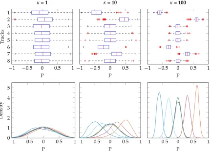
Three different values for κ were used, which illustrates how this parameter controls the

distribution of panning. The results are shown in Figure 10, where the influence of κ is clear.

When κ → 0, the distribution of pan positions approaches uniform over the sphere, and so the median pan positions are close to 0 (central position in the stereo field) for all tracks, regardless ofµpan. Asκ increases, the distribution of pan positions is narrower, more concentrated on the specific pan

positions specified inµpan.

Appl. Sci. 2017,7, x 12 of 23

This method involved generating random mono mixes as Section2.2(using Equation (7) and then generating pan positions separately. Aµpanwas created for a vMF distribution. This vector was based

on experimental results reported in [15], which showed that, generally, overheads and guitars were widely panned while kick, snare, bass and vocals were positioned centrally.

µpan

= [

−

0.5 0.5 0 0 0

−

0.4 0.4 0

]

(12)

This then needs to be a unit vector for it to be used in creating vMF-distributed points. Consequently, the precise values are not critically important, as it is the relative pan positions that are reflected in the normalised vector andrpanwhich would be used to adjust the scaling of these relative positions.

µpan

= [

−

0.5522 0.5522 0 0 0

−

0.4417 0.4417 0

]

(13)

Three different values for κ were used, which illustrates how this parameter controls the

distribution of panning. The results are shown in Figure 10, where the influence of κ is clear.

When κ

→

0, the distribution of pan positions approaches uniform over the sphere, and so the

median pan positions are close to 0 (central position in the stereo field) for all tracks, regardless ofµpan.

0.5 0 0.5 1

1 2 3 4 5 6 7 8

P

Tracks

κ= 1

−

1

−

0.5 0 0.5 1

0 1 2 3 4 5

P

[image:13.595.81.514.368.678.2]

Density

Figure 10.Panning method 2—generating vMF distributions in panning space. As expected, increasing

κ(concentration parameter) results in a narrower range of pan positions for each track, around the

target vector Equation (13).

Figure11shows an example of two mixes created using this method. The gains and pan positions of each track are displayed. It is clear that the instruments are typically panned close to the positions

Figure 10.Panning method 2—generating vMF distributions in panning space. As expected, increasing

κ(concentration parameter) results in a narrower range of pan positions for each track, around the

(14)

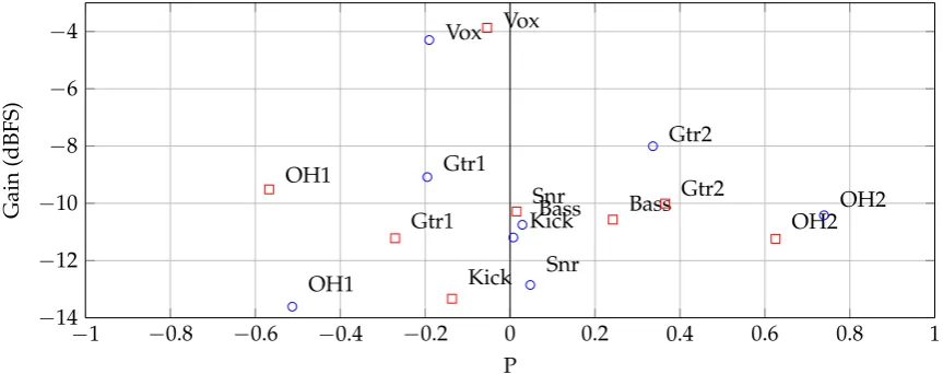
Figure11shows an example of two mixes created using this method. The gains and pan positions of each track are displayed. It is clear that the instruments are typically panned close to the positions specified in the pan vector (Equation (13). In this example,rpan=1; increasing this parameter would produce wider mixes, while a decrease would produce a less wide mix.

Appl. Sci. 2017,7, x 13 of 23

specified in the pan vector (Equation (13). In this example,rpan =1; increasing this parameter would produce wider mixes, while a decrease would produce a less wide mix.

−1 −0.8 −0.6 ₋0.4 −0.2 0 0.2 0.4 0.6 0.8 1

[image:14.595.83.515.158.329.2]

−14 −12 −10 −8 −6 −4 OH1 OH2 Kick Snr Bass Gtr1 Gtr2 Vox OH1 OH2 Kick Snr _Bass Gtr1 Gtr2 Vox P Gain (dBFS)

Figure 11.Two random mixes generated using panning method 2, shown as squares and circles. Each mix has a different gain vector (based on Equation (7) and different pan vector (based on Equation (13).

2.4. Track Equalisation

Similarly to how the mix can be considered as a series ofinter-channelgain ratios, when the frequency-response of a single audio track is split into a fixed number of bands, theinter-bandgain ratios can be used to construct atone-spaceusing the same formulae. For three bands, with gain of low, middle and high bands in the filter beingglow,gmidandghighrespectively, the problem is comparable to the 3-track mixing problem shown in Figure2a. Again, one can convert this to spherical coordinates (by Equations (5) and obtain[rEQ,ψ1,ψ2], yet, in this case, the values ofψncontrol the EQ filter applied, andrEQis the total amplitude change produced by equalisation (to avoid confusion,ψis used in place ofφwhen referring to equalisation). As before, if all three bands are increased or decreased by the

same proportion, then the tone of the instrument does not change apart from an overall change in presented amplitude,rEQ. Analogous to its use in track gains, the value ofψ2adjusts the balance betweengmidandghigh, whileψ1adjusts the balance ofglowto the previous balance.

g1,g2,g3, . . . ,gnbands

| {z }

gains of filter bands

= rEQ

|{z}

scaling

,ψ1,ψ2, . . . ,ψn−1

| {z }

tone-space

(14)

In Figure12, five points are randomly chosen in thetone-space. These co-ordinates are converted to three band gains as before, except that, in order to centre on a gain vector of[1, 1, 1],rEQ =√nbands, which is√3 in this example. Of course, this method can be used for any number of bands.

With this method, one must assume that an audio track has equal amplitude in each band, which is rarely the case. WhengLis increased on a hi-hat track, there may be little effect, compared to a bass guitar. Therefore, the loudness change is a function ofrEQand the spectral envelope of the track, prior to equalisation. This is not considered here and is left to further work.

Figure 11.Two random mixes generated using panning method 2, shown as squares and circles. Each mix has a different gain vector (based on Equation (7) and different pan vector (based on Equation (13).

2.4. Track Equalisation

Similarly to how the mix can be considered as a series ofinter-channel gain ratios, when the frequency-response of a single audio track is split into a fixed number of bands, theinter-bandgain ratios can be used to construct atone-spaceusing the same formulae. For three bands, with gain of low, middle and high bands in the filter beingglow,gmidandghighrespectively, the problem is comparable to the 3-track mixing problem shown in Figure2a. Again, one can convert this to spherical coordinates (by Equations (5) and obtain[rEQ,ψ1,ψ2], yet, in this case, the values ofψncontrol the EQ filter applied, andrEQis the total amplitude change produced by equalisation (to avoid confusion,ψis used in place ofφwhen referring to equalisation). As before, if all three bands are increased or decreased by the

same proportion, then the tone of the instrument does not change apart from an overall change in presented amplitude,rEQ. Analogous to its use in track gains, the value ofψ2adjusts the balance betweengmidandghigh, whileψ1adjusts the balance ofglowto the previous balance.

g1,g2,g3, . . . ,gnbands

| {z }

gains of filter bands

= rEQ

|{z}

scaling

,ψ1,ψ2, . . . ,ψn−1

| {z }

tone-space

(14)

In Figure12, five points are randomly chosen in thetone-space. These co-ordinates are converted to three band gains as before, except that, in order to centre on a gain vector of[1, 1, 1],rEQ =√nbands, which is√3 in this example. Of course, this method can be used for any number of bands.

(15)

[image:15.595.78.514.94.536.2]

Appl. Sci. 2017,7, 1329 14 of 21

Figure 12. Five randomly-chosen examples of 3-band equalisation, chosen from the tone-space. As ψ2 → 0, the gain of the high band decreases. As ψ1 → 0, the gain of the low band increases

at the expense of the other two bands; their balance is determined byψ2.

3. Applications

Being able to generate artificial datasets of audio mixtures in the mix-space has a variety of applications. Two such applications are described here. The procedure is similar for both experiments: an audio mix is created using a generated gain vector and raw multitrack audio, resulting in a generated mix from which audio signal features may be determined. Feature extraction used the MIRtoolbox [19], version 1.6.1. Equations (7) and (8) were used to create two sets of mixes. These experiments use sets of 500 mixes, rather than 1000 as outlined in earlier sections. It can be shown that the distributions of audio signal features do not change much beyond 500 mixes [15]. The reduced computation time is advantageous in these examples.

(16)

audio was reduced to the required eight tracks and each track was normalised in perceived loudness according to a modified form of ITU BS.1770 [20]. The songs “I’m Alright” and “What I Want” feature a track of piano as track #7, in place of ‘Gtr 2’.

3.1. Testing the Robustness of Tempo Estimation Algorithms to Changes in the Mix

In the absence of any time-stretching processes, the tempo of each mix should be identical for a given song. As a result, if the tempo of alternate mixes is estimated and any disagreement is found, this suggests limitations in the tempo-estimation algorithm. In this section, the process of estimating tempo across a large set of artificial mixes is presented as a means of assessing the performance of tempo-estimation algorithms. Two such algorithms are tested herein: the classic and metre-based [21] implementations of mirtempo in the MIRtoolbox. In short, the classic tempo estimation algorithm performs onset detection based on the amplitude envelope of the audio. Periodicities in the detected onsets are determined by finding peaks in the autocorrelation function. The metre method additionally takes into account the metrical hierarchy of the audio, allowing for a more consistent tempo-tracking. Whichever tempo-estimation is used, the resultant tempo is the mean value over the 30-second audio segment. Panning and equalisation were not considered here as tempo was estimated from a mono signal.

Figures13a and14a show the results for “Burning Bridges”, where it is clear that the classic method performs poorly. The correct tempo of 100 bpm is estimated for only a small percentage of the mixes while all others are estimated close to 133 bpm (see Figure14a). This leads to a high mean squared error (MSE) as shown in Table1. A similar flaw is evident for “I’m Alright” where the tempo is again overestimated by roughly 33% for both mix distributions (see Figures13b and14b). This indicates a consistent error in the tempo-estimation routine, which is being revealed by these mix distributions. The metre-based method performs much better, estimating the correct tempo in almost all cases and exhibiting a lower MSE, with only a small amount of absolute error (0.1–0.2 bpm). The performance of the classic tempo-estimation method is improved for “What I Want”, where both methods are found to have a high level of accuracy, as shown in Figures13c and14c. For both distributions, the metre-based version produces clusters of solutions for “What I Want”, although the tempo represented by largest cluster is consistent.

[image:16.595.140.456.585.672.2]

It is conceivable that no tempo-estimation algorithm is able to obtain the correct result in all cases. What this experiment reveals is that there is also variation within the mixes of a given song, with some mixes providing the correct tempo and other mixes yielding error, with different estimation methods showing varying levels of robustness to mixing practice.

Table 1.Summary of tempo estimation accuracy results. Shown is the mean squared error (MSE) in each set of 500 mixes.

Audio BPM Mixes Mirtempo (Classic) Mirtempo (Metre)

Burning Bridges 100 Equation (_{Equation (}7₈)₎ 998.54₁₀₈₂ _0.014713.05

I’m Alright 96 Equation (_{Equation (}7₈)₎ 738.4297_742.37 16.4854_16.7442

(17)

Appl. Sci. 2017,7, 1329 16 of 21

Appl. Sci. 2017,7, x 16 of 23

100 110 120 130

0 200 400

Estimated tempo (bpm)

Count

Classic method

50 60 70 80 90 100

0 200 400

Metre-based method

(a)

126.6 126.8 127 127.2 127.4 0

10 20

Count

Classic method

95.8 96 96.2 96.4 96.6 0

10 20 30

(b)

100 102 104 106

0 50 100 150

Count

Classic method

99.1 99.2 99.3 99.4 99.5 99.6 99.7 0

20 40

[image:17.595.105.490.88.513.2]

(c)

Figure 13.Estimated tempo for three songs, 500 mixes each using Equation (7). In each histogram, the data is split into 100 bins. Overall, performance is better for the metre-based method, as it demonstrates greater accuracy and improved robustness to changes in the mix. (a) “Burning Bridges”—The correct tempo is≈100 bpm; (b) “I’m Alright”—The correct tempo is≈96 bpm; (c) “What I Want”—The correct tempo is≈99 bpm.

Figure 13. Estimated tempo for three songs, 500 mixes each using Equation (7). In each histogram, the data is split into 100 bins. Overall, performance is better for the metre-based method, as it demonstrates greater accuracy and improved robustness to changes in the mix. (a) “Burning Bridges”—The correct tempo is ≈100 bpm; (b) “I’m Alright”—The correct tempo is ≈96 bpm; (c) “What I Want”—The correct tempo isAppl. Sci. 2017,7, x ≈99 bpm. 17 of 23

100 110 120 130

0 100 200 300

Count

Classic method

99.6 99.8 100 100.2 100.4 0

10 20

(a)

126.6 126.8 127 127.2 127.4 0

10 20

Count

Classic method

95.6 95.8 96 96.2 96.4 0

10 20

(b)

98.8 99 99.2 99.4 99.6 0

20 40

Count

Classic method

98.8 99 99.2 99.4 99.6 0

20 40

[image:17.595.110.489.602.732.2]

(c)

Figure 14. Estimated tempo for three songs, 500 mixes each using Equation (8). In each histogram, the data is split into 100 bins. Overall, performance is better for the metre-based method, as it demonstrates greater accuracy and improved robustness to changes in the mix; (a) “Burning Bridges”—The correct tempo is≈100 bpm; (b) “I’m Alright”—The correct tempo is≈96 bpm; (c) “What I Want”—The correct tempo is≈99 bpm.

3.2. Estimation of Spectral Centroid in Sets of Mixes

It is common to use the spectral centroid as a feature to describe the timbre of an audio signal, specifically as an approximation to perceptual brightness [22–24]. However, where the spectral centroid of a mixed recording is evaluated, it is not clear that the value obtained is typical of the recording as a whole, or if it simply relates to that specific mix of the recording. This is especially problematic in an object-based audio broadcast, where no reference mix exists. This applies to any signal feature, not just the spectral centroid. As studies of features across multiple alternate mixes are still rare in the literature [8,25,26], this issue has not been adequately investigated.

(18)

Appl. Sci. 2017,7, 1329 17 of 21

100 110 120 130 0

100 200 300

Count

Classic method

99.6 99.8 100 100.2 100.4 0

10 20

(a)

126.6 126.8 127 127.2 127.4 0

10 20

Count

Classic method

95.6 95.8 96 96.2 96.4 0

10 20

(b)

98.8 99 99.2 99.4 99.6 0

20 40

Count

Classic method

98.8 99 99.2 99.4 99.6 0

20 40

[image:18.595.111.481.87.359.2]

(c)

Figure 14. Estimated tempo for three songs, 500 mixes each using Equation (8). In each histogram, the data is split into 100 bins. Overall, performance is better for the metre-based method, as it demonstrates greater accuracy and improved robustness to changes in the mix; (a) “Burning Bridges”—The correct tempo is≈100 bpm; (b) “I’m Alright”—The correct tempo is≈96 bpm; (c) “What I Want”—The correct tempo is≈99 bpm.

Figure 14. Estimated tempo for three songs, 500 mixes each using Equation (8). In each histogram, the data is split into 100 bins. Overall, performance is better for the metre-based method, as it demonstrates greater accuracy and improved robustness to changes in the mix; (a) “Burning Bridges”—The correct tempo is ≈100 bpm; (b) “I’m Alright”—The correct tempo is ≈96 bpm; (c) “What I Want”—The correct tempo is≈99 bpm.

A previous work by the authors [8] reports on the spectral centroid of 1501 user-generated mixes of 10 songs. The number of mixes per song ranges from 97 to 373. The estimated probability distributions of spectral centroid are shown (among other signal features relating to amplitude, timbre and spatial properties), indicating that the median spectral centroid can vary by song, although it is still possible for significant overlap in distributions to exist.

The work in this section investigates the distributions of the spectral centroid that occur for artificial mixes drawn from different mix-space distributions. Equation (7) describes a simple model for mixes while Equation (8) shows the result of a perceptual level-balancing experiment. What is it about the mix that changes when these levels are adjusted? In this section, an estimation of the median spectral centroid produced by these two sets of mixes is made using Monte Carlo methods.

(19)

Appl. Sci. 2017,7, 1329 18 of 21

[image:19.595.130.469.143.644.2]

Figure15. These distributions were compared using a Wilcoxon rank sum test, which tests the null hypothesis that the distributions of both samples are equal. This null hypothesis was rejected in each case, as shown by thep-values in each subplot of Figure15(p<0.05 in each case).

Figure 15. Probability distribution of spectral centroid as a function of mix-space parameters; (a) “Burning Bridges”; (b) “I’m Alright”; (c) “What I Want”.

The significant difference between the medians of the two groups illustrates that there is a coarse perceptual difference in timbre, generally, between mixes drawn from the two distributions. This is true for all three songs considered. Of course, whether or not there is a significant difference between the medians of the two groups depends on the chosen parameters: theµvectors must be perceptually

different but ifκis low enough, then the distributions will overlap, regardless of the choice ofµ(recall that

(20)

The higher spectral centroid in the simple equal-gain-with-vocal-boost approach (Equation (7)) is caused by an overestimation in the level of the drum overheads and vocal, and an underestimation of the level of bass and kick drum, when compared to the results of the perceptual test (Equation (8)). The distributions of the spectral centroid for these artificially-generated mixes were compared to the distributions of the spectral centroid for user-generated mixes, as were reported in previous work by the authors [8]. For “Burning Bridges” and “What I Want”, the peak of theµinformeddistribution compares well to the user-generated mixes (approx 3.8 kHz and 3.2 kHz respectively). In the case of “I’m Alright”,µ =Equation (7) yields a better match to real mixes (approx 4.2 kHz); however, the 373 user-generated mixes of this song from [8] did contain a large proportion of highly amateur, potentially low-quality, mixes. For further comparison of artificial mixes and user-generated mixes, see [15].

This experiment shows that a set of mixes can be obtained by sampling the mix-space but that perceptually-relevant mixes are more likely to be obtained if some level of human guidance is fed into the system. The parametric mixing model for this experiment did not feature panning or equalisation. It has been shown that the addition of equalisation broadens the distribution of spectral centroid values, as would be expected given the wider variety of instrument tone [15].

4. Discussion

4.1. Artificial Datasets for Testing of Processes

The theoretical framework presented in this paper provides for a space of mixes that can be explored, using evolutionary computing, machine learning or similar computational methods. Applications of this include the creation of an initial population of solutions to be used in the search of balance-mixes [9] and electric guitar tones [10], both using interactive genetic algorithms. These approaches have yielded positive results, as the user is able to search the space effectively and find the desired solution.

For subjective testing, the methods presented in this paper have the advantage that each mix is generated at a constant perceived loudness, as the magnitude of the gain vector can be set to a constant (such asr=1 in Equation (4). In both [9,10], which used aninteractivegenetic algorithm, test participants were asked to rate subjectively the solutions presented. Being generated at a consistent loudness level allowed for fair evaluations, while avoiding the additional computational time required for specific loudness-normalisation to be applied to each generated mix. This allows a more free exploration of the solution space, since audio stimuli can be generated in real-time using this method.

Currently, newly-developed algorithms for tempo estimation, key estimation etc., are evaluated during specific challenges, such as the MIREX audio tempo estimation challenge ( http://www.music-ir.org/mirex/wiki/2017:Audio_Tempo_Estimation), using standard datasets of audio recordings. We propose that sets of artificially generated mixes be considered as a standard test, in order to examine the level of robustness to mixing practice, as in Section3.1.

4.2. Signal Analysis of Audio Mixing Practices

Of course, more conventional experiments can be analysed in this framework. In a level-balancing task, where participants were asked to set track gains to their desired levels, the resulting gains can be converted to the mix-space and analysed therein [7]. This allows differences in cohorts to be investigated: thus far, the different mixes produced by headphone or loudspeaker users has been investigated [15] in addition to checking if changing the initially presented rough mix influences the mixing-decisions [7], a hypothesis also supported by later work [6].