Operational matrix based on Genocchi polynomials for solution of delay differential equations

Operational matrix based on Genocchi polynomials for solution of delay

differential equations

Abdulnasir Isah, Chang Phang

⇑

Department of Mathematics and Statistics, Faculty of Science, Technology and Human Development, Universiti Tun Hussein Onn Malaysia, 86400 Batu Pahat, Johor, Malaysia

a r t i c l e i n f o

Article history: Received 15 July 2016 Revised 2 September 2016 Accepted 9 September 2016 Available online xxxx Keywords:

Genocchi polynomials

Operational matrix of derivatives Generalized pantograph equations Delay differential equations Collocation points

a b s t r a c t

In this paper, we present a new simple and effective algorithm for solving generalized Pantograph equa-tions, delay differential equations with neutral terms and delay differential system with constant and variable coefficients.The new method is based on one of the Appell polynomials, namely Genocchi poly-nomials. We first introduce the properties of Genocchi polynomials and employed them to construct the operational matrices of derivative. Collocation method based on this operational matrix is used. Error estimate for this scheme based on the Generalized pantograph equations is reproduced. Only few terms of Genocchi polynomials are needed to obtain very good results. Numerical examples with comparison show the simplicity, efficiency and accuracy of the method.

Ó2017 Ain Shams University. Production and hosting by Elsevier B.V. This is an open access article under the CC BY-NC-ND license (http://creativecommons.org/licenses/by-nc-nd/4.0/).

1. Introduction

Delay differential equations play an important role in explain-ing different phenomena in many different fields of study such as biology, physics, economics, electrodynamics, control theory etc. [1–3]. According to[2], the name pantograph refers to the device that collect electric current from overhead lines for electric trains or trams. The clear picture of this device is shown in[2]. The pan-tograph equations was originated from the work of Ockendon and Tayler[4]in which the system of collecting overhead electricity for trains is redesigned and modeled to ensure the contact is maintain throughout. Pantograph equations are fundamental when a phe-nomena or a process fail to be modeled by the ordinary differential equations. In recent years many researchers have focus in the numerical treatment of pantograph equations. Tohidi et al. in[5] proposed a new collocation scheme based on Bernoulli operational matrix for numerical solution of generalized pantograph equation. Yusufog˘lu[6]proposed an efficient algorithm for solving general-ized pantograph equations with linear functional argument. In [7]Yang and Huang presented a spectral-collocation method for fractional pantograph delay-integrodifferential equations and in [8], Yüzbasßi and Mehmet presented an exponential approximation for solutions of generalized pantograph delay differential

equations. Multiquadric approximation scheme was used in [9] for the numerical solution of delay differential systems of neutral type, Taylor method was used in [10] for numerical solution of generalized pantograph equations with linear functional argument. Chebyshev polynomials and Bessel polynomials are respectively used in[11,12]to obtain the solutions of generalized pantograph equations, while Adomian decomposition method and Variational iteration method are applied in [13,14] respec-tively for the solution of delay differential equations. In this paper, an important member of Appell polynomials called the Genocchi polynomials is used. Though Genocchi polynomials are not based on orthogonal functions but they possesses operational matrix of derivative and when it comes to function approximation, this poly-nomials share with other members of the Appell family, such as Bernoulli polynomials, some sound and advantageous properties over other classical orthogonal polynomials such as Legendre poly-nomials, Chebyshev polypoly-nomials, Laguerre polynomials and etc. These advantages are stated in[5].

Motivated by these advantages, we used Genocchi polynomials operational matrix of derivative through collocation method to approximate the solution of delay differential equation of pan-tograph type and those with neutral term together with its differ-ential systems. We based all our arguments on generalized form of pantograph equations given by[5]:

yðmÞ_{ðtÞ ¼}XI

i¼0 X m1

k¼0

pi;kðtÞyðkÞð

a

i;ktþbi;kÞ þgðtÞ; 06t61 ð1Þ

http://dx.doi.org/10.1016/j.asej.2016.09.015

2090-4479/Ó2017 Ain Shams University. Production and hosting by Elsevier B.V.

This is an open access article under the CC BY-NC-ND license (http://creativecommons.org/licenses/by-nc-nd/4.0/). Peer review under responsibility of Ain Shams University.

⇑ Corresponding author.

E-mail addresses:[email protected] (A. Isah),[email protected] (C. Phang).

Contents lists available atScienceDirect

Ain Shams Engineering Journal

subject to the following conditions

yj_{ð0Þ ¼d}

j; j¼0;1;. . .;m1: ð2Þ where

a

i;kandbi;kare real or complex coefficients, whilepi;kðtÞand

gðtÞare given continuous functions in the interval½0;1.

The rest of the paper is organized as follows: Section2, intro-duce some mathematical preliminaries of Genocchi polynomials. In Section 3, we apply the collocation method for solving pan-tograph Eq.(1)using the Genocchi operational matrix. Section4, we show the error analysis of the proposed method. In Section5, the proposed method is applied to several examples. Conclusion is given in Section6.

2. Some properties of Genocchi polynomials

Genocchi numbers and polynomials have been extensively studied in many different context in branches of mathematics such as elementary number theory and complex analytic number the-ory, in which this polynomials are highly developed and applied, like the so calledq-Genocchi polynomials are developed in[15– 17], their interpolation functions are also dicussed in [16,18]. Genocchi polynomials are also studied in homotopy theory (stable homotopy groups of spheres), differential topology (differential structures on spheres), theory of modular forms (Eisenstein series), and quantum physics (quantum groups). The classical Genocchi polynomialsGnðxÞis usually defined by means of the exponential generating functions[19–22].

2text

et_þ1¼ X1

n¼0

GnðxÞ

tn

n!; ðjtj<

p

Þ ð3Þ

whereGnðxÞis the Genocchi polynomials of degreenand is given by

GnðxÞ ¼ Xn

k¼0

n k Gkx

nk _ð4Þ

The first few Genocchi polynomials are;

G1ðxÞ ¼1

G2ðxÞ ¼2x1

G3ðxÞ ¼3x23x

G4ðxÞ ¼4x36x2þ1

G5ðxÞ ¼5x410x3þ5x

Differentiating both sides of(4), with respect tox, then we have the following as[21,23]

dGnðxÞ

dx ¼nGn1ðxÞ; nP1 ð5Þ

We prove one of the important property in the following Lemma

Lemma 2.1.

Gnð1Þ þGnð0Þ ¼0; n>1 ð6Þ

Proof.

From(3)we have that

ext_¼1

2t

2teðxþ1Þt

et_þ1 þ

2text

et_þ1

¼1 2t

X1

n¼0

Gnðxþ1Þ þGnðxÞ

ð Þtn

n!; ðjtj<

p

Þ

i.e. X1

n¼0

xn_tn

n! ¼

1 2t

X1

n¼0

Gnðxþ1Þ þGnðxÞ

ð Þtn

n!; ðjtj<

p

Þ ð7Þ

from(7)we have

Gnðxþ1Þ þGnðxÞ ¼2nxn1; n>1: ð8Þ Hence, the result follows obviously.h

If we introduce the Genocchi vector GðxÞ in the form

GðxÞ ¼ ½G1ðxÞ;G2ðxÞ;. . .;GNðxÞ, then the derivative of theGðxÞwith the aid of(5), can be expressed in the matrix form by

G0ðxÞT_¼

MGTðxÞ

where

G0ðxÞT_¼

G0₁ðxÞ

G02ðxÞ

G0₃ðxÞ

G0₄ðxÞ

... G0_N1ðxÞ

G0NðxÞ 0 B B B B B B B B B @ 1 C C C C C C C C C A

; M¼

0 0 0 0 0 0

2 0 0 0 0 0

0 3 0 0 0 0

0 0 4 0 0 0

... ... ... ... ... ...

0 0 0 N1 0 0

0 0 0 0 N 0

0 B B B B B B B B @ 1 C C C C C C C C A and

GðxÞT_¼

G1ðxÞ

G2ðxÞ

G3ðxÞ

G4ðxÞ

... GN1ðxÞ

GNðxÞ 0 B B B B B B B B B @ 1 C C C C C C C C C A

Thus,MisNNoperational matrix of derivative. Accordingly, thekth derivative ofGðxÞcan be given by

G0ðxÞT_¼

MGTðxÞ )Gð1ÞðxÞ ¼GðxÞMT

Gð2ÞðxÞ ¼Gð1ÞðxÞMT¼GðxÞðMTÞ2

Gð3ÞðxÞ ¼Gð1ÞðxÞðMTÞ2¼GðxÞðMTÞ3

... ... ...

GðkÞðxÞ ¼GðxÞðMTÞk

We refer to the work of E. Tohidi et al.[5]for the advantages of Appell family polynomials for approximating an arbitrary unknown function over some classical orthogonal polynomials.

3. Collocation method based on Genocchi operational matrix

In this section, we use the collocation method based on Genoc-chi operational matrix of derivatives to solve numerically the gen-eralized pantograph equation. We now derive an algorithm for solving(1). To do this, let the solution of(1)be approximated by the firstNterms Genocchi polynomials. Thus, we write

yNðxÞ XN

n¼1

cnGnðxÞ ¼GðxÞC ð9Þ

where the Genocchi coefficient vectorCand the Genocchi vector

GðxÞare given by

CT¼ ½c1;c2;. . .;cN; GðxÞ ¼ ½G1ðxÞ;G2ðxÞ;. . .;GNðxÞ

then, thekth derivative ofy_NðxÞcan be expressed as follows

yðNkÞðxÞ ¼G

ðkÞ_{ðxÞC¼GðxÞðM}T_Þk

C ð10Þ

Substituting(9) and (10)in(1)we have

GðtÞðMTÞmC¼X

I

i¼0 X m1

k¼0

pi;kðtÞGð

a

i;ktþbi;kÞðM T_Þk

CþgðtÞ ð11Þ

whereGð

_a

i;ktþbi;kÞ ¼ ½G1ð

a

i;ktþbi;kÞ;G2ð

a

i;ktþbi;kÞ;. . .GNð

a

i;ktþbi;kÞ. Also the initial condition will producemother equations

Gð0ÞðMT_Þj_C¼d

j j¼0;1;. . .;m1 ð12Þ To find the solutionyNðxÞ, we collocate(11)at the collocation pointstj¼_Njm,j¼1;2;. . .;Nmto obtain

GðtjÞðMTÞ m

C¼X

I

i¼0 X m1

k¼0

pi;kðtjÞGð

a

i;ktjþbi;kÞðM

T_Þk_Cþgðt

jÞ ð13Þ

for j¼1;2;. . .;Nm. (13) are Nm non-linear algebraic equa-tions. These equations together with(12)makeNalgebraic equa-tions which can be solved using Newton’s iterative method. ConsequentlyyNðxÞgiven in(9)can be calculated.

4. Error analysis

Suppose thatH¼L2_{½0;1and G}

1ðtÞ;G2ðtÞ;. . .;GNðtÞ

f g Hbe the

set of Genocchi polynomials andY¼Span Gf 1ðtÞ;G2ðtÞ;. . .;GNðtÞg. Also letfðtÞbe arbitrary element ofH, sinceYis a finite dimen-sional subspace,fðtÞhas a unique best approximation in Y, say

fðtÞsuch that8yðtÞ 2Y;kfðtÞ fðtÞk26kfðtÞ yðtÞk2.

Since fðtÞ 2Y, then there exist the unique coefficients

c1;c2;. . .;cNsuch that

fðtÞ fðtÞ ¼X

N

n¼1

cnGnðtÞ ¼CGðtÞ

whereC¼ ½c1;c2;. . .;cN; GðtÞ ¼ ½G1ðtÞ;G2ðtÞ;. . .;GNðtÞ

In the following Lemma we prove a new way that shows how the coefficientscncan be obtained.

Lemma 4.1.Assume that f2H¼L2½0;1, is an arbitrary function approximated by the truncated Genocchi seriesPNn¼1cnGnðxÞ, then the

coefficients cnfor n¼1;2;. . .;N can be calculated from the following

relation

cn¼

1 2n!ðf

ðn1Þ_{ð1Þ þf}ðn1Þ_ð0ÞÞ:

Note that the power inðn1Þinfðn1ÞðxÞdenotes theðn1Þth derivative off

Proof.SupposefðxÞ PN

n¼1cnGnðxÞ, then, using(6)one has

fð1Þ þfð0Þ ¼c1ðG1ð1Þ þG1ð0ÞÞ þc2ðG2ð1Þ þG2ð0ÞÞ þ þcN ðGNð1Þ þGNð0ÞÞ ¼2c1

)c1¼ 1

2ðfð1Þ þfð0ÞÞ

fð1Þð1Þ þfð1Þð0Þ ¼2c2ðG1ð1Þ þG1ð0ÞÞ þ3c3ðG2ð1ÞþG2ð0ÞÞ þ þNcN ðGN1ð1Þ þGN1ð0ÞÞ ¼2c2ð2Þ

)c2¼ 1 2ð2!Þðf

ð1Þ_{ð1Þ þf}ð1Þ_ð0ÞÞ

fð2Þð1Þ þfð2Þð0Þ ¼3ð2Þc3ðG1ð1Þ þG1ð0ÞÞ þ þNðN1ÞcNðGN2ð1Þþ

GN2ð0ÞÞ ¼3ð2Þc3ð2Þ

)c3¼ 1 2ð3!Þðf

ð2Þ_{ð1Þ þ}

fð2Þð0ÞÞ

Repeating this procedureitimes fori¼1;2;. . .;N, we have

ci¼

1 2i!ðf

ði1Þ_{ð1Þ þf}ði1Þ_ð0ÞÞ;

this complete the proof.h

Theorem 4.2. Suppose that fðxÞ 2C1½0;1and fðtÞis the approxi-mated fðtÞby using Genocchi polynomials, then the error bound would be obtained as follows;

kerrorðfðtÞÞk₁6 1 N!GNFN

where GN and FN denotes the maximum value of GNðtÞ and

fðN1ÞðtÞ 8t2 ½0;1respectively.

Proof. The proof is obvious, one should considerLemma 4.1.h In the following we reproduced the theorem given in[5]which gives an upper bound for the error of the considered problem(1)

Theorem 4.3. Let yðxÞ and yNðxÞ be the exact and approximate solutions of (1) respectively. Consider (1) when m¼1 so that piðtÞ ¼pi;kðtÞ. Also assume that 8t2 ½0;1;kyðtÞk16

q

;kKiðtÞ k₁¼ kpið

tbi

aiÞk16Ki; i¼1;2;. . .;I and

PI

i¼1ðKiþEKiÞ–1, then

kyðtÞ yNðtÞk16

Ef þ

q

PI

i¼1EKi 1PIi¼1ð

K

iþEKiÞ

;

whereEKi¼ kKiðtÞ Ki;NðtÞk1,i¼1;2;. . .;IandEf ¼ kfðtÞ fNðtÞk1, withfðtÞ ¼yð0Þ þRt

0gð

s

Þd

s

.

Proof. According to the assumptions above(1)becomes:

y0ðtÞ ¼X

I

i¼0

piðtÞyð

a

itþbiÞ þgðtÞ

Integrating both sides in the interval ½0;t and imposing initial condition we have

yðtÞ ¼yð0Þ þ

Z t

0

gð

s

Þd

s

þX

I

i¼0 Z t

0

pið

s

Þyð

a

i

s

þbiÞd

s

yðtÞ ¼fðtÞ þX

I

i¼0 Z t

0

pið

s

Þyð

a

i

s

þbiÞd

s

puttingz¼

a

i

s

þbi, we get,

yðtÞ ¼fðtÞ þX

I

i¼0 Z _aitþbi

bi 1

a

i

pið

zbi

a

i

ÞyðzÞdz

If we assumeKiðzÞ ¼piðz

bi

aiÞthe above equation can be written as:

yðtÞ ¼fðtÞ þX

I

i¼0 Z _aitþbi

bi 1

a

i

KiðzÞyðzÞdz:

Now, suppose that the functionsKiðzÞandfðtÞare expanded in terms of Genocchi polynomials, then the obtained solutionyNðxÞis also in terms of Genocchi polynomials. Our aim here is to find an upper bound for the associated error between the exact solution

yðxÞand the approximated solutionyNðxÞfor Eq.(1). With consid-ered assumptions we have;

kyðtÞ yNðtÞk1¼ kfðtÞ fNðtÞ þ XI

i¼0 Z _aitþbi

bi 1

a

i

ðKiðzÞyðzÞ

Ki;NðzÞyNðzÞÞdzk1

6kfðtÞ fNðtÞk1þ

XI

i¼0 Z _aitþbi

bi j1

a

i

j kðKiðzÞyðzÞ

Ki;NðzÞyNðzÞÞk1dz

kKiðzÞyðzÞ Ki;NðzÞyNðzÞk1¼ kKiðzÞyðzÞ KiðzÞyNðzÞ þKiðzÞyNðzÞ

Ki;NðzÞyNðzÞk1

6kKiðzÞk1kyðzÞ yNðzÞk1þ kKiðzÞ

Ki;NðzÞkðkyðzÞ yNðzÞk1þ kyðzÞk1Þ

Thus, putting this in the last result we get

kyðtÞ yNðtÞk16Efþ XI

i¼0

ð

K

iþEKiÞkyðtÞ yNðtÞk1þ

q

XI

i¼0

EKi

Hence,

kyðtÞ yNðtÞk16

Efþ

q

PI

i¼0EKi 1PIi¼0ð

K

iþEKiÞ

:

This complete the proof.h

5. Numerical examples

In this section, some numerical examples are given to illustrate the applicability and accuracy of the proposed method. All the numerical computations have been done using Maple 18.

Example 5.1. Let us first consider the second order pantograph equation[5,6,13]

y00ðtÞ ¼3 4yðtÞ þy

t 2 t

2_{þ2; t2 ½0;1: ð14Þ}

subject to

yð0Þ ¼0; y0ð0Þ ¼0

The exact solutions of this problem is known to beyðtÞ ¼t2_{[6]. We} apply our technique withN¼3. Approximating(14)with Genocchi polynomials we have:

GðtÞðMTÞ2C¼3

4GðtÞCþG t 2 Ct

2_{þ2 ð15Þ}

Also from the initial conditions we have

Gð0ÞC¼0 and Gð0ÞðMTÞC¼0 ð16Þ

Thus, collocating(15)att¼3 4, we get

57 8 c3

7 4c1

1 8c2

23 16¼0

From the initial conditions we havec1c2¼0 and 2c23c3¼0. Solving this three equations we have

c1¼ 1 2; c2¼

1 2; c3¼

1 3

Thus,yðtÞ ¼GðxÞCis calculated and we havex2_{which is the exact} solution. This result is the same as in[5]We also compare the dif-ference between the exact solution and numerical solutions obtained by[6,13]and present method inTable 1

Example 5.2.We consider the following pantograph equation[10]

y0ðtÞ ¼1 2e

t 2y t

2 þ 1

2yðtÞ; t2 ½0;1: ð17Þ

subject to

yð0Þ ¼1

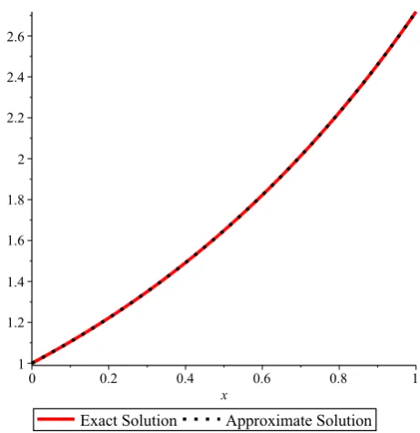
The exact solution of this problem is known to beyðtÞ ¼et_{. We} solve(17)using our technique withN¼15. The solution obtained by our method is in good agreement with the exact solution as shown inFig. 1. The absolute error obtained by our method is com-pared with that obtained in[10]as shown inTable 2.

Example 5.3. Consider the following non linear third order pantograph equation

y000ðtÞ ¼ 1þ2y2 t

2 t2 ½0;1: ð18Þ

subject to

yð0Þ ¼0; y0ð0Þ ¼1 y00ð0Þ ¼0

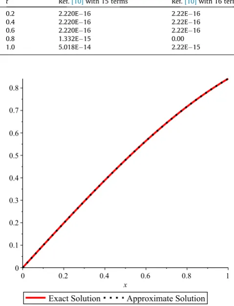
[image:4.595.310.541.393.631.2]

The exact solution of(18)is known to beyðtÞ ¼sinðtÞwhich we solve using our technique withN¼15. We compare our result with those obtained using HPM in[6], eight terms of the series have been used which means the terms are up tot15_{. Hence, in} our method we usedN¼15.Fig. 2, also confirm that our solution is in good agreement with the exact solution (seeTable 3).

Table 1

Comparison of approximate solution obtained by[6,13]and present method with exact solution forExample 5.1.

t Ref.[13], 13 terms Ref.[6], 8 terms Present method, 3 terms (N= 3) Exact solution

0.2 0.04 0.04 0.04 0.04

0.4 0.16 0.16 0.16 0.16

0.6 0.36 0.36 0.36 0.36

0.8 0.64 0.64 0.64 0.64

1.0 1.00 1.00 1.00 1.00

Fig. 1.Comparison of our solution with the exact solution forExample 5.2.

[image:4.595.31.553.694.757.2]

Example 5.4. Here we consider the delay equation with neutral term[14]

y0ðtÞ ¼ yðtÞ þ1 2y

t 2 þ

1 2y

0 t

2 t2 ½0;1: ð19Þ

subject to

yð0Þ ¼1

The exact solution of this problem is given byyðtÞ ¼et_{. We} used present method to solve (19)with N¼8;11. The absolute error obtained by our method is compared with that obtained in [14]as shown inTable 4.

Note that inTable 4,mandNstands for the number of terms of the polynomials used for evaluating the approximate solution of the problem

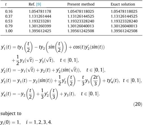
[image:5.595.48.559.86.149.2]

Example 5.5. Finally we consider the following neutral delay differential system[9]

Table 4

Comparison of absolute errors obtained by[14]and present method forExample 5.4

t Ref.[14],m= 8 Present method,N= 8 Present method,N= 11 Present method,N= 15

0.2 7.08E4 9.614E8 6.055E12 4.133E18

0.4 1.29E3 1.047E7 6.380E12 4.251E18

0.6 1.76E3 1.007E7 6.061E12 3.990E18

0.8 2.15E3 9.338E8 5.554E12 3.629E18

[image:5.595.45.285.92.405.2]

1.0 2.47E3 8.563E8 4.980E12 3.237E18

Table 2

Comparison of absolute errors obtained by[10]and present method forExample 5.2

t Ref.[10]with 15 terms Ref.[10]with 16 terms Present method, withN= 15 Present method withN= 16

0.2 2.220E16 2.22E16 3.318E18 7.7855E20

0.4 2.220E16 2.22E16 4.051E18 9.5066E20

0.6 2.220E16 2.22E16 4.948E18 1.1611E19

0.8 1.332E15 0.00 6.044E18 1.4181E19

[image:5.595.312.563.332.394.2]

1.0 5.018E14 2.22E15 7.339E18 1.7414E19

Fig. 2.Comparison of our solution with the exact solution for example5.3.

Table 3

Comparison of the Exact solution and approximate solution obtained by[6]and our method forExample 5.3.

t Ref.[6] Present method Exact solution

0.2 0.19866933079506122 0.19866933079506121678 0.19866933079506122 0.4 0.38941834230865050 0.38941834230865049281 0.38941834230865050 0.6 0.56464224733950355 0.56464247339503535809 0.56464224733950355 0.8 0.71735609089952280 0.71735609089952276216 0.71735609089952280 1.0 0.84147109848078965 0.84147098480789650670 0.84147109848078965

Table 6

Comparison of the Exact solution and approximate solutiony2ðtÞobtained by[9]and our method forExample 5.5

[image:5.595.291.562.465.527.2]

t Ref.[9] Present method Exact solution 0.16 1.173510870 1.17351087099 1.17351087099 0.37 1.447734613 1.44773461466 1.44773461466 0.53 1.698932307 1.69893230861 1.69893230861 0.79 2.203396425 2.20339642625 2.20339642625 1.00 2.718281828 2.71828182846 2.71828182846 Table 5

Comparison of the Exact solution and approximate solutiony1ðtÞobtained by[9]and our method forExample 5.5.

[image:5.595.111.491.575.637.2] [image:5.595.41.562.693.756.2]

y01ðtÞ ¼ty1

t

2 ty2 sin

t 2

þcosðtÞy02ðsinðtÞÞ

þ1 2y3ð

ffiffi

t p

Þ y03ð ffiffi

t p

Þ; t2 ½0;1;

y02ðtÞ ¼ y1ð ffiffi

t p

Þ þy2ðtÞ þy02ðsinð ffiffi

t p

ÞÞ; t2 ½0;1;

y03ðtÞ ¼y1ðtÞ y2ðsinðtÞÞ þ 1 2y

0

2

t 2

t 3y3

2t 3 þty

0

4ðtÞ; t2 ½0;1;

y04ðtÞ ¼ y2

t 2 þ

1 3y

0

2

t

3 þy3ðtÞ; t2 ½0;1:

ð20Þ

subject to

yið0Þ ¼1; i¼1;2;3;4:

The exact solution of this problem is given by y1ðtÞ ¼esinðtÞ;

y2ðtÞ ¼et; y3ðtÞ ¼e

t 2 and y

4ðtÞ ¼e

t

3 We solve this system using our technique withN¼15. The solution obtained by[9]and our method are compared with the exact solution inTables 5–8. This comparison indicates that our method gives more accurate results.

6. Conclusion

In this paper, a collocation method based on the Genocchi oper-ational matrix for solving generalized pantograph equations is pre-sented. The comparison of the results shows that the present method is an excellent mathematical tool for finding the numerical solutions delay equation. The advantage of the method over others is that it has less computational complexity because every operational matrix of differentiation involves more numbers of zeroes and thus, reduces the run time and provide the solution at high accuracy.

Acknowledgements

This work was supported in part by FRGS Grant Vot 1433. We also thank for financial support from UTHM through GIPS U060.

References

[1]Aiello WG, Freedman HI, Wu J. Analysis of a model representing stage-structured population growth with state-dependent time delay. SIAM J Appl Math 1992;52(3):855–69.

[2]Dehghan M, Shakeri F. The use of the decomposition procedure of Adomian for solving a delay differential equation arising in electrodynamics. Phys Scripta 2008;78(6):065004. Nov 19.

[3]Kuang Y, editor. Delay differential equations: with applications in population dynamics. Academic Press; 1993. Mar 5.

[4]Ockendon J, Tayler AB. The dynamics of a current collection system for an electric locomotive. Proc Roy Soc Lond A: Math Phys Eng Sci 1971;322(1551). The Royal Society, May 4.

[5]Tohidi E, Bhrawy AH, Erfani K. A collocation method based on Bernoulli operational matrix for numerical solution of generalized pantograph equation. Appl Math Model 2013;37(6):4283–94. Mar 15.

[6]Yusufog˘lu E. An efficient algorithm for solving generalized pantograph equations with linear functional argument. Appl Math Comput 2010;217 (7):3591–5. Dec 1.

[7]Yang Y, Huang Y. Spectral-collocation methods for fractional pantograph delay-integrodifferential equations. Adv Math Phys 2013;2013. Nov 20. [8]Yüzbasßi Sß, Sezer M. An exponential approximation for solutions of generalized

pantograph-delay differential equations. Appl Math Model 2013;37 (22):9160–73. Nov 15.

[9]Vanani SK, Aminataei A. Multiquadric approximation scheme on the numerical solution of delay differential systems of neutral type. Math Comput Model 2009;49(1):234–41. Jan 31.

[10]Sezer M, Akyüz-DasßcÄs´oglu A. A Taylor method for numerical solution of generalized pantograph equations with linear functional argument. J Comput Appl Math 2007;200(1):217–25. Mar 1.

[11]Sedaghat S, Ordokhani Y, Dehghan M. Numerical solution of the delay differential equations of pantograph type via Chebyshev polynomials. Commun Nonlinear Sci Numer Simul 2012;17(12):4815–30. Dec 31. [12]Yüzbasßi Sß, Sßahin N, Sezer M. A Bessel collocation method for numerical

solution of generalized pantograph equations. Numer Methods Partial Differ Eqs 2012;28(4):1105–23. Jul 1.

[13]Evans DJ, Raslan KR. The Adomian decomposition method for solving delay differential equation. Int J Comput Math 2005;82(1):49–54. Jan 1.

[14]Chen X, Wang L. The variational iteration method for solving a neutral functional-differential equation with proportional delays. Comput Math Appl 2010;59(8):2696–702. Apr 30.

[15]Kim T. On the q-extension of Euler and Genocchi numbers. J Math Anal Appl 2007;326(2):1458–65. Feb 15.

[16]Cangul IN, Ozden H, Simsek Y. A new approach to q-Genocchi numbers and their interpolation functions. Nonlinear Anal: Theory Methods Appl 2009;71 (12):e793–9. Dec 15.

[17]Cangul IN, Kurt V, Ozden H, Simsek Y. On the higher-order w-q-Genocchi numbers. Adv Stud Contemp Math 2009;19(1):39–57.

[18]Srivastava HM, Kurt B, Simsek Y. Some families of Genocchi type polynomials and their interpolation functions. Integral Transforms Special Funct 2012;23 (12):919–38. Dec 1.

[19]Araci S. Novel identities forq-Genocchi numbers and polynomials. J Function Spaces Appl 2012;2012. Jul 24.

[20]Araci S. Novel identities involving Genocchi numbers and polynomials arising from applications of umbral calculus. Appl Math Comput 2014;233:599–607. May 1.

[21]Horadam AF. Genocchi polynomials. In: Proceedings of the 4th international conference on Fibonacci numbers and their applications. Kluwer Academic; 1991. p. 145–66.

[22]Ozden H, Simsek Y, Srivastava HM. A unified presentation of the generating functions of the generalized Bernoulli, Euler and Genocchi polynomials. Comput Math Appl 2010;60(10):2779–87. Nov 30.

[23]Araci S, Sßen E, Acikgoz M. Theorems on Genocchi polynomials of higher order arising from Genocchi basis. Taiwanese J Math 2014;18(2):473. Mar 21.

[image:6.595.33.283.95.157.2]

Abdulnasir Isah obtained his PhD in 2017 from University Tun Hussein Onn Malaysia. He recieved his Bs.c in Mathematics from Bayero University Kano Nigeria with first class honor. He teaches Mathematics at the department of mathematics Ahmadu Bello University zaria, Nigeria. His research interests are in the areas of fractional differential equations and their application.

Table 7

Comparison of the Exact solution and approximate solutiony3ðtÞobtained by[9]and our method forExample 5.5

[image:6.595.32.285.205.425.2]

t Ref.[9] Present method Exact solution 0.16 1.083287066 1.08328706767 1.08328706767 0.37 1.203218439 1.20321844012 1.20321844012 0.53 1.303430975 1.30343097577 1.30343097577 0.79 1.484384190 1.48438419092 1.48438419092 1.00 1.648721270 1.64872127070 1.64872127070

Table 8

Comparison of the Exact solution and approximate solutiony4ðtÞobtained by[9]and our method forExample 5.5

t Ref.[9] Present method Exact solution 0.16 1.054781178 1.05478118025 1.05478118025 0.37 1.131261444 1.13126144525 1.13126144525 0.53 1.193233281 1.19323328240 1.19323328240 0.79 1.301260399 1.30126040013 1.30126040013 1.00 1.395612425 1.39561242508 1.39561242508

Chang Phangis senior lecturer at Universiti Tun Hussein Onn Malaysia. He received the PhD degree in Mathe-matics and Statistics at Curtin University, Australia. His research interests are in the areas of differential equa-tions, specifically in fractional differential equations and application in some mathematical biology.