Should the Neoclassical growth model include the saving flow in the Utility function?

Munich Personal RePEc Archive

Should the Neoclassical growth model

include the saving flow in the Utility

function?

Khelifi, Atef

ECONETRIX Consulting

15 November 2014

Online at

https://mpra.ub.uni-muenchen.de/59751/

Should the Neoclassical growth model include the saving

flow in the Utility function?

Atef Khelifi*

Abstract

Despite ‘joy of giving models’ have been extensively examined in the literature, the Ramsey growth model has never been explored under the assumption of a direct

preference for bequeathing savings that are reinvested. This assumption implies a

Utility function depending on both consumption and savings, which may also be

motivated as one that captures a direct preference for thriftiness or wealth

accumulation arguably involved. The resulting growth model generalizes those

accounting for the capitalist spirit as Zou (1994), and shows that the restrictive

standard one is perhaps not the actual optimized version of the Solow model.

JEL O41, E21, D91

Keywords: Bequest; Status; Anticipatory feelings; Ramsey growth model

* _{ECONETRIX Consulting, Paris, France, [email protected], Tel: +33 (0)1.85.06.77.98}

“The difficulty lies not in the new ideas, but in escaping the old ones, which ramify, for those brought up as most of us have been, into every corner of our minds.”

J.M.Keynes, New York 1987.

1.Introduction

It goes to our mind almost systematically, that the flow of saving should never be included in

the Utility function along with consumption, to solve the inter-temporal maximization problem of

the consumer. Two reasons can be stated precisely and may sound a bit obvious only at first

glance. The first one which is to consider savings as having no intrinsic value for the individual,

can arguably be contested in some cases. The second, a technical redundancy deduced from

standard conceptions, can be shown to be misleading, especially in models of accumulation. The

goal of this paper is to criticize the systematic neutrality of a Utility effect of savings in the

literature, and to report the relevant implications in the Ramsey growth model where specifically,

such neutrality is perhaps inappropriate.

To contest the first reason for excluding savings from Utility in the Ramsey context, it might

not be necessary to recall the capitalist spirit literature motivating that individuals derive direct

Utility from wealth accumulation for the status; see for example Weber (1930), Zou (1994),

Bakshi and Chen (1996), or Carroll (2000). Indeed, by introducing the saving flow in the Utility

function, not only is the continual seek for a higher capital and status captured, but also a direct

preference for thriftiness which could be involved if the individual worries about the necessity to

renovate the depreciated capital, or to accumulate sufficient wealth for the growing household.1

In life-cycle (LC) or overlapping generations (OLG) models, the neutrality of this direct

preference for thriftiness or wealth accumulation is systematically constrained every period, such

that the individual saves only to defer own consumption in the future when ‘profitable’. Because

of this particularity, alternative models accounting for the bequest motive have been proposed in

the literature. One type includes for example Barro (1974) or Laitner (1992), where successive

generations working for only one period value the level of Utility of their children. Another

consists in “joy of giving models” like for example Andreoni (1990), or more recently Dynan,

Skinner and Zeldes (2002), where individuals gain satisfaction from bequeathing a part their

1 _{This idea can be related to the modern literature of anticipatory feelings, like for example Kuznitz, Kandel and Fos (2008). The individual is} supposed conscious and can be affected in the present by future situations, even under a deterministic context. In our case, the thrifty individual

lifetime income to the children. Although the second type has been extensively examined in the

literature, the altruistic Ramsey model has never been explored under the assumption of a direct

preference for bequeathing savings that are reinvested. It could be supposed for example, that

each generation working at period t cares about saving for renovating or increasing the capital left

to the children at t+1, before retiring or eventually dying. From this conceptual viewpoint, a

direct preference for saving finds a very strong motivation in that framework, aside from a

plausible preference for thriftiness or wealth accumulation.

Technically, it may have seemed redundant at first glance to introduce explicitly this preference

in the model, because the time preference rate already measures the relative preference for

current consumption, and the dynamics is already such that savings and accumulation occur when

the interest rate exceeds this time preference rate. However, the time discounter is precisely

defined by Samuelson (1937) as a degree of impatience that reflects the relative preference for

current well-being2, and the standard dynamics is specific to the lifetime utility function which corresponds by construction to one of a LC model in an infinite-horizon case. Assuming a direct

preference for saving or accumulating generates a more general dynamics, which also extends

those of models accounting for the capitalist spirit as Zou (1994). Furthermore, it allows to

recover logically the basic static properties of the exogenous Solow version.

Similarly to growth models involving absolute wealth in Utility as Zou (1994), or relative

wealth as Corneo and Jeanne (2001), the presented model allows to invest more than in the

standard version by modulating the preference for wealth accumulation. This property is known

as a plausible way to contrast with the contested lower boundary condition and convergence

theorem of the traditional theory. It implies for instance that necessary and sufficient conditions

required to meet the golden rule of accumulation can be specified. Another similarity that might

also be important to report, is that the effect of the natural growth rate of workers on the

steady-state level of capital per capita appears confirmed. Those common results could eventually be

interpreted as two steps already made towards a reconciliation with Solow’s static properties of

the steady-state.

In contrast with this previous literature however, the proposed preference function generates a

slower transition, and offers the possibility to reach also lower steady-state levels of capital per

2

capita than in the standard model by investing less. Aside from allowing to recover a total

coherence with the basic exogenous version, this second property might complement

explanations of cross-country differences, and for instance, reconcile more empirical growth facts

of developing countries with optimal growth theory.

The proposed Ramsey model is not presented as an augmented version of the standard one

only, or as a generalization of capitalist spirit growth models, but as being perhaps an appropriate

formulation that could have been missed because of an eventual misunderstanding of the

preference for saving. Given such properties of the results indeed, nothing really precludes the

possibility that the standard model assumes an unsuitable Utility function to optimize the Solow

version. Precisely, it could for example be necessary to clarify first the goal of the individual in

the exogenous model, before deciding which preferences would be more appropriate. Does this

individual want to consume or to accumulate wealth, when choosing a constant saving rate 𝑠 ∈

(0,1)? If the answer is ‘both’, which of those two alternatives is most preferred by this ‘saver’?

The remainder is organized as follows. Section 2 presents conditions under which it might be

relevant to introduce savings in Utility. Section 3 shows that applying this type of preferences in

the Ramsey model appears to generate more consistent results than in the standard case. Section 4

concentrates on a discussion of the transition through a comparative analysis, and Section 5

concludes.

2. A Further Formulation of Preferences

It is highly important to justify in details why individuals could derive direct Utility from

saving. The first section presents what is meant by a direct preference for thriftiness and wealth

accumulation. The second concerns ‘joy of bequeathing’.

A. Preference for Thriftiness and Wealth

According to its generic definition, the concept of Utility which measures satisfaction or

welfare is of course not limited to consumption and leisure; examples in the literature are indeed

gifts, cash-holding or wealth. As soon as a particular individual endowed of personal preferences

gains satisfaction from actions decided among a set of alternatives, then such actions could

eventually be arguments of a Utility function of this individual. For example, an individual could

individual appreciates to be thrifty, is out of the microeconomic field and relies completely on

personal reasons it takes as given. Perhaps, it is not necessarily a Utility function including a

saving effect that needs to be justified, but eventually the assumption that all individuals can

never feel (instantaneously) better by saving instead of consuming; one evidence that indeed

contradicts this assumption is at least miserliness (under an extreme case.)

More particularly, some reasons could be exposed to defend the relevance of controlling a

saving (or investment) utility effect in neoclassical growth models.

The conceptual logic of the Solow model is to involve a thrifty agent who saves each time a

part of income to accumulate or renovate capital in the long run. It could be plausible to consider

that saving (or investing) causes this individual to feel immediately better because, (i) it removes

bad anticipatory feelings like anxiety or sadness if future wealth appears insufficient for some

reasons (welfare of children, renovation of capital, job loss, illness, retirement, bequests, etc.); (ii)

enhancing wealth is a way to achieve a higher social status, as argued for example by Weber

(1930) who defines this desire as the spirit of capitalism.

In real life indeed, reasons why individuals decide to save or invest are not necessarily

economic. Admittedly, some of the reasons are either psychological or sociological. It may not be

surprising therefore if the traditional theory involving an agent who derives Utility from the act of

consuming only, appears limited when applied to real data. For instance, Kenneth Arrow also

said in 1988:

“The dominant paradigm was that people essentially saved to spend in their lifetime.

But today the evidence seems to be accumulating that this hypothesis is not true, and

everybody seems to agree that you cannot explain savings solely on a life cycle basis

[…] So to conclude, I think that the key thing when it comes to the relationship between

economics and sociology is the willingness to look at new kinds of data, like in savings. I

think that once you do that, you are automatically going to be forced to consider social

elements. Just ask different questions, and I think you are going to be forced into

considering and drawing upon sociology.”

(Stanford University, April 1988).

Many research works in various fields of the literature have incorporated factors affecting

bequests, gifts, and more recently, social status and anticipatory feelings. Notable works follow

respectively Yaari (1965), Barro (1974), Andreoni (1990), Zou (1994), and Kuznitz, Kandel and

Fos (2008).

In the neoclassical growth framework, a direct preference for the stock of capital has been

introduced by Zou (1994) to formalize the spirit of capitalism of Max Weber3_{, and proved to be}

relevant for the explanation of several empirical growth facts. In contrast, Corneo and Jeanne

(2001) have proposed to account for the relative amount of wealth instead, by suggesting that

individuals care about their relative position in a society. In the presented paper, an alternative

way to formalize the continual seek for a higher status is proposed through a saving (or

investment) effect in the flow of Utility, meaning that individuals value the growing of wealth (or

capital) each time, rather than the absolute or relative stock itself.

Aside from the status motive or anticipatory feelings, earlier literatures have already considered

the possibility for individuals to derive Utility from gifts or bequests. It might be worth

discussing implications of ways to characterize the intergenerational altruism in the Ramsey

growth model.

B. Joy of Bequeathing

Traditional inter-temporal maximization problems of the consumer might be separated into two

major categories. The first one includes LC or OLG models as developed by Modigliani and

Brumberg (1954), Modigliani (1986), Diamond (1965), etc. The second is constituted of altruistic

or inter-dependent generations’ models as in Barro (1974), Laitner (1992), Yaari (1965), etc.

In the first case, each generation derives utility only from own lifetime consumption and

dissaves, or ‘plans’ to dissave, entirely during retirement. The second case mainly includes

models where life-cycle utility can also, either be affected by the welfare of children, or by the

act of giving or bequeathing (which gave the name of ‘joy-of-giving’ or ‘warm glow’ to this

literature).

Recall now the conceptual approach of the altruistic Utility proposed by Barro (1974) that

serves as a basis to the standard Ramsey model. Assuming each generation lives for only two

periods, utility of individuals born at time t is expressed as:

3

(1) 𝑉_𝑡= 𝑈_𝑡+ 𝛾𝑉_𝑡+1,

where 𝑉_𝑡 denotes total Utility of parents, 𝑈_𝑡 is the Utility from life-cycle consumption (of both

periods), 𝑉_𝑡+1 is the total Utility of children, and 𝛾 is the discounting factor that measures the

degree of altruism. Substituting recursively all Utilities up to generation T, gives the following

dynastic function:

(2) 𝑉_𝑡 = ∑𝑇−1_𝑗=𝑡 𝛾𝑗−𝑡𝑈_𝑡+ 𝛾𝑇−𝑡𝑉_𝑇,

where the term 𝛾𝑇−𝑡𝑉_𝑇 vanishes as T tends to infinity. In other words, the resulting specification

simplifies by construction to one of a LC model in the infinite horizon case. Under this

assumption, the optimal rule which governs saving decisions is such that individuals save to defer

consumption only when profitable; ie. only when interest opportunities are more valuable than

current consumption. In the standard Ramsey model particularly, properties of the production

technology are such that the agent finds optimal to save and to accumulate up to an equilibrium

level when starting from below, and to disaccumulate when departing from above. Recalling that

the time discounting factor is technically bounded downward by the natural growth rate in that

framework, the inevitable consequence is that the household is ‘condemned to poverty’ if

marginal productivity of capital, as the unique driving force of the accumulation process, happens

unfortunately to be low. Many research works in endogenous growth theory have tried to escape

this constraining rule or ‘lower boundary condition’ by assuming different production

technologies, but as suggested by Zou (1994), it seems reasonable to revise preferences as well,

and to admit that individuals could still decide to invest more and grow under such unfavorable

conditions.

An alternative conceptual approach to the lifetime Utility of an altruistic household, is one

which separates Utility from giving, and Utility from the well-being of children which depends

on their own total income at time t+1. For instance, the previous Utility of a generation born at

time t could be expressed as:

where 𝑐_𝑡 is consumption and 𝑠_𝑡 is the bequest. This intergenerational ‘transfer’ of income might

be a convenient way to measure the degree of altruism in the Ramsey framework, alternatively to

the time discounting factor only. In that case, the bequest reflects the desire to renovate or to

increase the capital stock left to the children at time t+1, before retiring or eventually dying.

Interestingly, this idea may apply to various examples in real life. Aside from business or private

concerns indeed, the natural environment could also be assimilated as a productive capital for

which (insufficient) investments and efforts are made today, in order to preserve it for the

children and future generations.

3. A Further Formulation of the Ramsey Growth Model

The first section presents the model which involves an interesting application of the

Pontryagin’s Maximum Principle. The second discusses the steady-state and Golden Rule.

A. The Optimal Control Program

At time t, a representative generation composed of L workers cares about consuming and

reinvesting a part of income produced. The instantaneous preference function is defined by

𝑈𝑡(𝑐𝑡, 𝑠𝑡), where 𝑐𝑡 denotes per capita consumption at t, 𝑠𝑡 denotes per capita savings (or

bequests), and 𝜃 ∈ (0,1) is a proportion which measures the degree of preference for

consumption over savings. The budget constraint of this representative agent is given by 𝑐_𝑡+

𝑠𝑡 = 𝑦𝑡, where 𝑦𝑡 denotes income per worker. The production function is supposed of the

Cobb-Douglas form with constant returns to scale, such that 𝑦_𝑡 = 𝑓(𝑘_𝑡) = 𝑘_𝑡𝛼, where 𝑘_𝑡 denotes capital

per worker, and 𝛼 ∈ (0,1). The dynastic Utility function (after substitution of 𝑠_𝑡) is denoted by

𝑉{𝑐𝑡, 𝑘𝑡}. It is maximized over an infinite horizon subject to a dynamic constraint of capital

accumulation (by the social planner):

(4) Max

𝑐𝑡 𝑉{𝑐𝑡, 𝑘𝑡} = ∫ 𝑈𝑡(𝑐𝑡, 𝑘𝑡) 𝑒

(𝑛−𝛽)𝑡_𝑑𝑡 ∞

𝑡0 ,

where 𝑛 is the natural growth rate of workers, 𝛽 is the usual degree of impatience and 𝛿 is the

rate of depreciation of capital. We impose the usual restriction 𝛽 > 𝑛 to ensure a feasible interior

solution to the problem.

Some interesting steps of the resolution are worth presenting. For the sake of concreteness, we

assume a Cobb-Douglas Utility function 𝑈_𝑡(𝑐_𝑡, 𝑠_𝑡) = 𝑐_𝑡𝜃𝑠_𝑡1−𝜃 and its log-transformation

𝑈𝑡(𝑐𝑡, 𝑠𝑡) = 𝜃ln(𝑐𝑡) + (1 − 𝜃)ln(𝑠𝑡).

Considering the first specification for example, the Hamiltonian is given by:

(6) 𝐻_𝑡(𝑐_𝑡, 𝑠_𝑡) = 𝑐_𝑡𝜃[𝑓(𝑘_𝑡) − 𝑐_𝑡]1−𝜃𝑒(𝑛−𝛽)𝑡+ 𝜆_𝑡𝑒(𝑛−𝛽)𝑡[𝑓(𝑘_𝑡) − 𝑐_𝑡− (𝑛 + 𝛿)𝑘_𝑡],

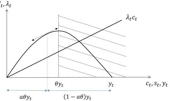
Following the Pontryagin’s Maximum principle, the first order condition implies 𝜕𝑈𝑡⁄𝜕𝑐𝑡 =𝑈𝑐𝑡 = 𝜆𝑡, which means that the static maximization of 𝐻𝑡 is satisfied under the following conditions:

𝑐𝑡 = 𝜃𝑓(𝑘𝑡) 𝑖𝑓 𝜆𝑡 = 0

𝑐𝑡 ∈ [0; 𝜃𝑓(𝑘𝑡)[ 𝑖𝑓 𝜆𝑡 > 0

The Pontryagin’s method requires to substitute a maximizing condition in the expressions that

serve to derive the dynamic equation of the control. In our case, the homothetic property of the

instantaneous Utility function allows us to define a convenient maximizing condition by letting

𝑎 ∈ (0,1) such that4_:

𝜆𝑡 = (𝑐_𝑠𝑡_𝑡) 𝜃

(1−𝑎_𝑎 ) ≥ 0 and 𝑐𝑡 𝑠𝑡=

𝑎𝜃 1−𝑎𝜃

Letting 𝑓_𝑘=𝜕𝑓(𝑘𝑡)

𝜕𝑘𝑡 , the second condition implies:

(7) (1 − 𝜃)𝑐_𝑡𝜃𝑠_𝑡−𝜃𝑓_𝑘+ 𝜆_𝑡(𝑓_𝑘− 𝛽 − 𝛿) = −𝜆̇_𝑡,

4_{An excellent reference explaining substitutions of Pontryagin’s maximizers is H.Schättler and U.Ledzewicz (2012), p.96. Techn}

A standard resolution that involves the substitution of equation (5) and static equilibrium values

of the co-state and ratio defined above, leads to the dynamic equation of consumption

𝑐𝑡̇ (𝑐𝑡, 𝑘𝑡, 𝑎). To simplify notations, we will omit the arguments.

The resulting differential system is:

(8) 𝑐̇_𝑡 =1−𝑎𝜃

1−𝜃 [(2 − 𝑎𝜃 − 𝜃)𝑓𝑘− (1 − 𝑎)(𝛿 + 𝛽)]𝑐𝑡− 𝑎𝜃(𝑛 + 𝛿)𝑓𝑘𝑘𝑡,

𝑘̇_𝑡 = 𝑓(𝑘_𝑡) − 𝑐_𝑡− (𝑛 + 𝛿)𝑘_𝑡.

In clear, there can be multiple dynamical systems depending on the value of 𝑎 ∈ (0,1), which

satisfy the first necessary conditions. This means that among all admissible values of 𝑎, or 𝜆_𝑡 as

explained by Schättler and Ledzewicz (2012), it remains to determine which one(s) maximize(s)

𝑉𝑡{𝑐𝑡∗, 𝑘𝑡∗}. In that sense, we may now define 𝑎 as being a choice parameter associated to a set of

controlled trajectories, and 𝑎∗ as being the rational choice associated to the optimal one which

maximizes total welfare.

Contrary to the differential equation of consumption (8), the one of the log-transformed Utility

can admit the value of 𝜃 = 1, in which case it simplifies to the standard Ramsey equation. Its

expression is given by:

(9) 𝑐𝑡̇

𝑐𝑡=

1−𝑎𝜃

1+𝑎𝜃(𝑎−2)[2𝑎(1 − 𝜃)𝑓𝑘+ (1 − 𝑎)(𝑓𝑘− 𝛽 − 𝛿)] −

𝑎(1−𝜃)

1+𝑎𝜃(𝑎−2)(𝑛 + 𝛿)𝛼,

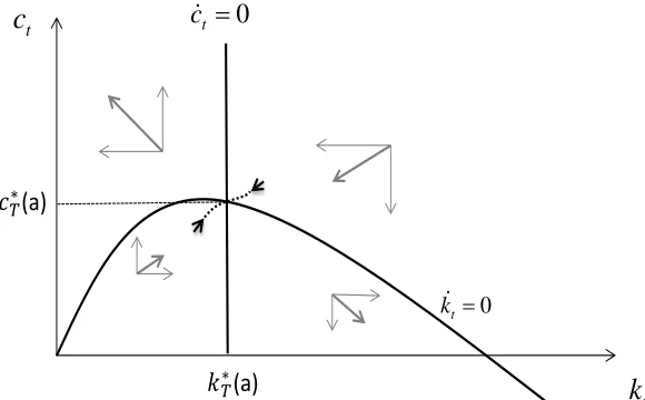
The graphical resolution of the dynamical systems shows that for any 𝑎 ∈ (0,1), there exists a unique saddle path in each case leading to a steady state equilibrium denoted by {𝑐_𝑇∗(𝑎), 𝑘_𝑇∗(𝑎)}. The phase diagram corresponding to the multiplicative Cobb Douglas case (figure 1), shows that

the parameter a affects only the convexity of the ‘𝑐_𝑡̇ = 0 locus’5. The level of consumption increases to the left of this locus, and decreases to the right. For the case of the log-Utility (figure

2), the phase diagram is identical to the standard one except that the vertical ‘𝑐𝑡̇ = 0 locus’

depends now on the parameter 𝑎.

5

Figure 1. Phase Diagram for the Multiplicative Cobb-Douglas Case

Figure 2. Phase Diagram for the Additive Cobb-Douglas Case

Let {𝑐_𝑡∗(𝑎), 𝑘_𝑡∗(𝑎)} denote any equilibrium (or saddle path) solution that leads to the steady-state at 𝑡 = 𝑇. It can easily be noticed that the transversality condition lim

𝑡→∞𝜆𝑡(𝑎)𝑘𝑡

∗_(𝑎)𝑒(𝑛−𝛽)𝑡_{= 0, is}

fulfilled at equilibrium if 𝛽 > 𝑛 because:

lim

𝑡→∞𝜆𝑡(𝑎) = 𝑈𝑐𝑇∗(𝑎), from the first necessary condition,

lim

𝑡→∞𝑘𝑡∗(𝑎)𝑒(𝑛−𝛽)𝑡= 𝑘𝑇∗(𝑎). lim𝑡→∞𝑒(𝑛−𝛽)𝑡= 0, if 𝛽 > 𝑛. t

c

t

k



t

k

(a)

if a < 1 0



t

c

0 

t

c if

t

c

t

k



t

k

(a) (a)

0



t

Let the control set be defined by:

𝑍 = {𝑐𝑡∗(𝑎) ∈ ℝ++ / 𝑐𝑡∗(𝑎) < 𝑦𝑡∗(𝑎) ∀ 𝑎 ∈ (0,1)},

such that total welfare 𝑉_𝑡{𝑐_𝑡∗(𝑎), 𝑘_𝑡∗(𝑎)} is restricted to the set of real numbers. We can now

proceed to a formal definition of a feasible optimal solution to the problem.

PROPERTY 1: An admissible controlled trajectory {𝑐_𝑡∗(𝑎∗), 𝑘_𝑡∗(𝑎∗)} satisfying the necessary

Pontryagin’s conditions ∀ 𝑎∗ ∈ (0,1), 𝑐_𝑡∗(𝑎∗) ∈ 𝑍 and 𝑘_𝑡∗(𝑎∗) ∈ ℝ++, is an optimal controlled trajectory if and only if 𝑉_𝑡{𝑐_𝑡∗(𝑎), 𝑘_𝑡∗(𝑎)} ≤ 𝑉_𝑡{𝑐_𝑡∗(𝑎∗), 𝑘_𝑡∗(𝑎∗)} ∀ 𝑎 ∈ (0,1) / 𝑎 ≠ 𝑎∗, 𝑐_𝑡∗(𝑎) ∈

𝑍, 𝑘_𝑡∗(𝑎) ∈ ℝ++.

An important result to keep in mind, is that the rational choice of the optimal trajectory is

determinant for the terminal steady-state {𝑐_𝑇∗(𝑎∗), 𝑘_𝑇∗(𝑎∗)} reached in the long run.

B. Steady-states and Golden Rule

Contrary to the multiplicative Cobb Douglas Utility function, the log form allows to derive a

steady-state solution analytically, which is:

(10) 𝑘_𝑇∗(𝑎) = [ (1−𝑎𝜃)(1−2𝑎𝜃+𝑎)𝛼

𝑎(1−𝜃)(𝑛+𝛿)𝛼+(1−𝑎𝜃)(1−𝑎)(𝛽+𝛿)] 1 (1−𝛼)

.

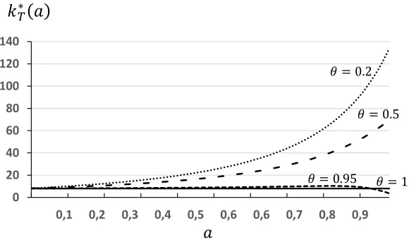
For any non-corner point (𝜃, 𝑎) ∈ (0,1) × (0,1), the steady-state level of capital (or income) per worker is a decreasing function of the natural growth rate. Hence, as soon as individuals are

assumed to gain some Utility from accumulating or saving, the negative impact of population

growth known from the basic exogenous Solow model is recovered.

There might be two reasons why this result should actually be defended. First, it seems

reasonable to expect that an optimized version of the Solow model, which goal focuses only on

producing an endogenous saving or investment rate along the transition, should preferably

Second, it is well known that ‘wealth-dilution’ is one effect of population growth that has been widely admitted and confirmed empirically; for example, Mankiw, Romer and Weil (1992) might

be one of the most influential contribution in that sense. It seems therefore counterfactual to

admit that the negative impact of high fertility is entirely compensated by an increase in the

investment-output ratio, as predicted by the standard Ramsey model.

Another important static property that plays a crucial role for the dynamics is the one of the

golden rule from Phelps (1961). The Ramsey growth model, as it is used in most macroeconomic

studies, is characterized by a steady-state level of capital per worker that remains always lower

than the consumption maximizing level (and hence, than the over-accumulation one as well). As

explained previously, this constitutes one of the reasons why alternative capitalist spirit models

have been proposed in the literature, following for example Zou (1994) and Corneo and Jeanne

(2001). Before presenting necessary and sufficient conditions for a golden rule steady-state, it

may be preferable to present first a more general property that concerns any ‘terminal’ or

constrained steady-state.

PROPERTY 2: Among all feasible controlled trajectories {𝑐_𝑡∗(𝜃, 𝑎), 𝑘_𝑡∗(𝜃, 𝑎)} ∈ 𝑍 × ℝ++, converging to a particular steady-state solution { 𝑐̅̅̅̅ , 𝑘_𝑇∗ ̅̅̅̅ }_𝑇∗ , there exists a preference-choice couple (𝜃∗, 𝑎∗) ∈ (0,1) × (0,1) compatible with an optimizing behavior; ie. which satisfies:

𝑉𝑡{𝑐𝑡∗(𝜃, 𝑎), 𝑘𝑡∗(𝜃, 𝑎)} ≤ 𝑉𝑡{𝑐𝑡∗(𝜃∗, 𝑎∗), 𝑘𝑡∗(𝜃∗, 𝑎∗)}, ∀ (𝜃, 𝑎) ∈ (0,1) × (0,1) / (𝜃, 𝑎) ≠ (𝜃∗, 𝑎∗)

This property resulting directly from the resolution might be viewed as a reciprocal of the first

one. Indeed, a steady-state dynamics is an optimal controlled trajectory as soon as there is no

other ways to reach the same dynamics with a higher total welfare. Suppose for example that the

constrained terminal state corresponds to the solution of the Solow model:

𝑘_𝑇∗

̅̅̅̅ = (𝑠̅̅̅𝑇∗

𝑛+𝛿)

1 1−𝛼

where 𝑓_𝑘̅̅̅̅_𝑇∗ =(𝑛+𝛿)𝛼_𝑠 𝑇∗

̅̅̅ and 𝑠̅̅̅ ∈ (0,1)𝑇∗

steady-states. Under cases where both sets offer potential candidates however, the terminal state

assumed can possibly be generated by two different optimal trajectories (or two different rational

behaviors). In such a multiple equilibrium context, the goodness of fit to real data may lastly

decide.

The golden rule steady-state which maximizes consumption is reached if 𝑠̅̅̅_𝑇∗ = 𝛼. For the multiplicative Cobb-Douglas form, the following condition must hold:

(11) [1 + 1−𝜃

(1−𝑎𝜃)𝑋𝑎𝜃(𝑛 + 𝛿)] −1

= 𝛼,

where 𝑋 = (2 − 𝑎𝜃 − 𝜃)(𝑛 + 𝛿) − (1 − 𝑎)(𝛿 + 𝛽), and for the log-Utility case,

(12) 1−𝑎𝜃

𝑎(1−𝜃)[1 + 𝑎(1 − 2𝜃) − (1 − 𝑎) 𝛽+𝛿 𝑛+𝛿] = 𝛼.

4. Numerical Analysis of the Dynamics

This section presents results of numerical simulations. The analysis focuses on the additive log

Utility function with no loss of generality concerning the Cobb Douglas form. Following the first

property, the first part analyzes the dynamics of the optimal path. The second addresses the

question of recovering this path starting from a given steady-state. It also compares the dynamics

with those of standard growth models and the one proposed by Zou (1994).

A. General Properties of the Dynamics

The question that comes first is to know how total welfare changes with respect to the

parameter a, which has been defined previously as reflecting the choice of an admissible

trajectory made by the individual. The next interesting step is to understand how the variables

behave along the optimal path6_.

Numerical simulations show that for a preference parameter 𝜃 that tends to one, the optimal

value of 𝑎 decreases and the maximum total welfare tends to stabilize for 𝑎 < 𝑎∗. In figure 3 for

example, when 𝜃 = 0.95, the maximum total welfare attains 𝑉∗ = 241.62 at 𝑎∗= 0.71, and

remains almost constant for 𝑎 ≤ 0.71 (precisely, it decreases slowly until 𝑉 = 241.36 at 𝑎 =

6 _{Numerical computations of saddle paths are made according to the shooting method. A solution 𝑎}∗ _{is considered sufficiently accurate if in its}

neighborhood, changes in total welfare become relatively negligible. In this part, parameters kept constant are assigned the following values: 𝛼 =

0.01). As 𝜃 decreases, the value of 𝑎∗ increases but at a much lower rate; for instance 𝑎∗ = 0.76 when 𝜃 = 0.85 and 𝑎∗= 0.78 when 𝜃 = 0.2. This figure shows also that the choice of the right

equilibrium co-state (or value of a) matters much more for lower values of 𝜃. For example, the

size of the welfare gain from an admissible path to the optimal one can exceed 26% in the case

where 𝜃 = 0.2.

Figure 3. Total Welfare by Admissible Path

Figure 4. Steady-state Per Capita Capital by Admissible Path

Another result that figure 3 illustrates, is that individuals with different degrees of preference

for saving (or bequeathing) face different levels of total welfare. When 𝜃 remains relatively high,

total welfare is lower than in the standard case where individuals value consumption only. As 𝜃

200 210 220 230 240 250 260

0,1 0,2 0,3 0,4 0,5 0,6 0,6 0,7 0,8 0,9

0 20 40 60 80 100 120 140

decreases below a certain cutoff value, total welfare tends to increase back until reaching higher

values than in the standard model. Besides the fact that the steady-state saving rate for such

values of 𝜃 seems unreasonable, as indicated by figure 6, this parameter describing fixed

preferences is conceptually not to be ‘selected’ so that total welfare or even consumption is

maximized7.

In figure 4, it is interesting to notice that accounting for supplementary (social) motives for

saving, does not always mean a higher steady-state capital per capita than in the standard model.

For values of 𝜃 that are close to one (0.95 in our example), there are some admissible trajectories

(for high values of a) which lead to lower steady-state capital per capita than in the standard case.

This interesting remark will be developed later.

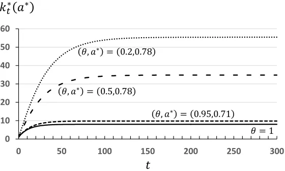
Concerning transitions towards higher-steady-states, figure 5 shows that (unconstrained)

optimal trajectories exhibit a faster growth when preferences for saving for social reasons become

more intense. Interestingly, although the speed of growth increases with such intense preferences,

thrifty individuals appear less sensitive to variations of the interest rate compared to those who

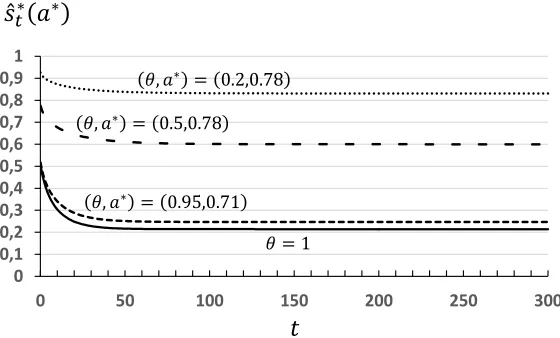
care about consumption only. For instance, figure 6 shows that the magnitude of the variation of

the saving rate along the optimal path increases with 𝜃.

Figure 5. Equilibrium Path of Capital Per Capita

7

The golden rule of capital accumulation is indeed not necessarily what individuals prefer. 0

10 20 30 40 50 60

Figure 6. Equilibrium Path of the Saving Rate

B. Dynamics in Constrained Optimization Cases

Suppose for example that individuals are endowed of preferences for consuming and

bequeathing such that future generations benefit from the golden rule steady-state at time T,

where consumption is maximized.

It is well known that for this steady-state to be possible under the standard altruistic case, the

flow of Utility must be augmented to include a direct preference for wealth (or status) as for

example in Zou (1994). A general specification widespread in this literature is:

(13) 𝑊{𝑐_𝑡, 𝑘_𝑡} = ∫ [𝑢_𝑡∞ _𝑡(𝑐_𝑡) + 𝑣_𝑡(𝑘_𝑡)] 𝑒(𝑛−𝛽)𝑡𝑑𝑡

0 ,

where 𝑣_𝑡(𝑘_𝑡) represents the part of utility derived from the capital stock, with 𝑣_𝑘 > 0 and 𝑣_𝑘𝑘< 0. Preserving same notations as in the presented paper, the resolution of the program under this

assumption leads to the following rule:

(14) 𝑓_𝑘𝑇 = 𝛿 + 𝛽 −𝑣𝑘

𝑢𝑐,

0 0,1 0,2 0,3 0,4 0,5 0,6 0,7 0,8 0,9 1

Hence, given the ratio 𝑣𝑘⁄_𝑢𝑐 is always positive, the steady-state capital per capita in such models

will always be greater than in the standard one. The alternative Utility function proposed in this

paper generates a more general version of the neoclassical growth model by contrasting this

result.

For a convenient comparative analysis, suppose the flow of Utility of the capitalist spirit model

of Zou (1994) is given by:

(15) 𝑢_𝑡(𝑐_𝑡) + 𝑣_𝑡(𝑘_𝑡) = 𝑙𝑛(𝑐_𝑡) + 𝛾𝑙𝑛(𝑘_𝑡), where 𝛾 ∈ [0, ∞).

For 𝑛 = 0, it can be shown that the steady-state capital per capita is given by:

(16) 𝑘_𝑇 = ( 𝛼+𝛾

(𝛾+1)𝛿+𝛽) 1 1−𝛼

,

and is increasing in γ. The value of this parameter can be easily deduced such as to meet the

golden rule steady-state.

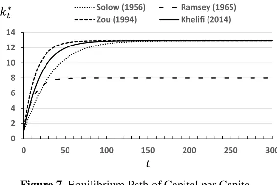
Figure 7. Equilibrium Path of Capital per Capita

Notes: Common parameters in each model are assigned the following values:𝛼 = 0.3, 𝛽 = 0.02, 𝑛 = 0, 𝛿 = 0.05, 𝑘₀= 1. The steady-state saving rate associated to the golden rule is therefore 0.3. In the presented model, the optimal pair (𝜃, 𝑎∗) is deduced accordingly and equals (0.901,0.85) and in the model of Zou (1994), 𝛾 = 0.171. The standard Ramsey results have been included in each figure to compare the dynamics; the steady-state level of the saving rate 𝑠̂_𝑇∗ equals 0.21 in that model.

0 2 4 6 8 10 12 14

0 50 100 150 200 250 300

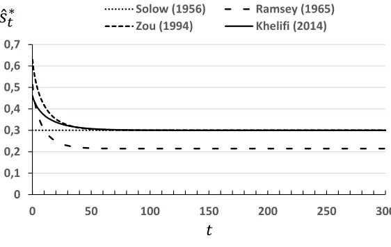
Figure 8. Equilibrium Path of the Saving Rate

Notes: Common parameters in each model are assigned the following values:𝛼 = 0.3, 𝛽 = 0.02, 𝑛 = 0, 𝛿 = 0.05, 𝑘₀= 1. The steady-state saving rate associated to the golden rule is therefore 0.3

The slowest transition towards the golden rule steady-state in figure 7 and 8, is unsurprisingly

the Solow one where individuals do not benefit from highest returns initially. In all other cases,

an optimal decision implies a faster speed of growth which differs depending on the type of

preferences assumed. It appears clearly that the model of Zou (1994) generates the faster

transition. In other words, the stock of capital in the Utility function, compared to the

unconsumed part of income, affects more intensively the willingness to accumulate.

Clearly, it is not possible a priori, or theoretically, to determine which one of those augmented

versions of the Ramsey model ensures a superior fit to empirical data. However, every common

parameters equal, the proposed model offers the possibility to adjust a slower dynamics towards

the same steady-state.

An additional particularity of the proposed model shown by figure 4, is to allow for some

admissible controlled trajectories towards lower steady-states as well. Departing from the

standard model, this figure indicates that the steady-state level of capital per capita increases with

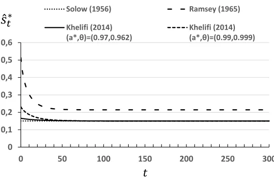
the degree of preference for saving (1 − 𝜃)and with the choice parameter 𝑎, except for few cases where (1 − 𝜃) is relatively low. Figures 9 and 10 present an example of transition towards a lower steady-state. For a ‘terminal’ saving rate 𝑠̂_𝑇∗ of 0.15 (versus 0.21 in the standard model), two different optimal trajectories are possible. In both cases, the speed of growth remains

logically greater than in the Solow model. For the case where the value of 𝜃 is higher, the

corresponding value of ‘𝑎’ leading to the specified steady-state with the maximum welfare is also

0 0,1 0,2 0,3 0,4 0,5 0,6 0,7

0 50 100 150 200 250 300

higher and very close to one. Interestingly, the difference between the values of 𝑎 in each case is such that the trajectory of the individual endowed of the higher preference for consumption 𝜃, appears faster than the one who values wealth accumulation more intensively. In that case, the

thriftiest individual is again less sensitive to variations of capital returns.

Figure 9. Equilibrium Path of Capital Per Capita

Notes: Common parameters in each model are assigned the following values:𝛼 = 0.3, 𝛽 = 0.02, 𝑛 = 0, 𝛿 = 0.05, 𝑘₀= 1. The steady-state saving rate in the Solow model and in the presented one equals 0.15. Two solutions (𝜃_𝑖, 𝑎_𝑖∗) are compatible with an optimizing behavior towards this steady-state, (0.999,0.99) and (0.962,0.97). The standard Ramsey results are reported for comparisons (in this model, 𝑠̂_𝑇∗= 0.21).

Figure 10. Equilibrium Path of the Saving Rate

Notes: Common parameters in each model are assigned the follow values:𝛼 = 0.3, 𝛽 = 0.02, 𝑛 = 0, 𝛿 = 0.05, 𝑘₀= 1. The steady-state saving rate in the Solow model and in the presented one equals 0.15

0 2 4 6 8 10

0 50 100 150 200 250 300

Solow (1956) Ramsey (1965)

Khelifi (2014) (a*,θ)=(0.97,0.962)

Khelifi (2014) (a*,θ)=(0.99,0.999)

0 0,1 0,2 0,3 0,4 0,5 0,6

0 50 100 150 200 250 300

Solow (1956) Ramsey (1965)

Khelifi (2014) (a*,θ)=(0.97,0.962)

The constrained optimization case should perhaps not be interpreted as one where the

representative household targets the terminal steady-state to reach. Instead, it should simply be

considered as a convenient way to recover the utility function under the assumption of rationality

from the observed empirical data. It might eventually be more useful in cases of relatively low

steady-states like in developing countries, where households can be exposed to constraints

regarding their saving or investment capacities.

5. Conclusion

Is the individual in the Solow model a ‘consumption-lover’ with a saving rate of 50%? Is the preference for accumulating implicitly involved in growth models, and should it be taken into

account independently from personal motives (power, influence, thriftiness, miserliness, gifts,

bequests, etc.)?

No matter what answers are, the standard model generates a steady-state level of capital per

capita bounded by the golden rule level, where the resulting equilibrium saving rate reaches a

maximum value of ‘𝛼’ (roughly estimated at 30%), when the time preference rate tends to its lower bound level n. Another apparent weakness of this model, is that it predicts the

counterfactual result of a wealth-dilution effect totally absorbed by a reduction in the

consumption share.

Capitalist spirit growth models as proposed for example by Zou (1994), offer a reasonable way

to contrast these constraining and counterfactual properties. However, the love of wealth

accumulation as formalized in such models, allows to extend the set of possible dynamics to

efficient and over-accumulation ones only, so that explanations of low GDP levels remain limited

to the time preference rate essentially. If adjusting the time preference rate in the standard model

has been inappropriate to explain differences among ‘rich countries’, and if controlling some additional willingness to invest has proved necessary, then it seems reasonable to admit that same

extensions are required for low GDP countries. The proposed model offers the possibility to

expand the set of steady-states on both sides of the standard version, so that eventual poverty

traps characterized by insufficient investment can also be reconciled in a same way with optimal

growth theory.

Several issues that have been investigated in the literature on the basis of the standard Ramsey

arguably more realistic. An additional advantage that might motivate the use of this model

particularly, concerns the context of an open-economy. Indeed, it is well-known that the standard

dynamics presents the counterfactual result of a consumption and wealth that tend to zero in an

open-economy where the time preference rate exceeds the world interest rate; see for example

Barro and Sala-i-Martin (1995, chapter 3). A recent suggestion from Hof and Wirl (2008) to

overcome this problem, is to augment the Utility function by including absolute or relative wealth

as an argument. Besides the fact that this type of preferences might still be restrictive, as

explained in this paper, the initial level of capital must be greater than a lower bound level to

ensure a possible accumulation towards a steady-state where both capital and consumption are

greater than zero. Such a condition is not required in the proposed model which offers a simpler

framework.

REFERENCES

Andreoni, James. “Impure Altruism and Donations to Public Goods: A Theory of Warm-Glow

Giving.” Economic Journal, June 1990, 100, pp.464-477.

Bakshi, Gurdip; Chen Zhiwu. “The Spirit of Capitalism and Stock-Market Prices.” American Economic Review, March 1996, 86 (1), 133-57.

Barro, Robert. “Are Government Bonds Net Wealth?” Journal of Political Economy, December

1974, 82(6), pp. 1095-1117.

Barro & Sala-i-Martin. “Economic Growth.” Mc Graw Hill, 1995.

Caroll, Christopher. “Why do the Rich Save so Much?” Does Atlas Shrug? The Economic

Consequences of Taxing the Rich, Ed. by Joel B. Slemrod, Harvard University Press, 2000, pp.

465-484

Cornero, Giacomo; Jeanne, Olivier. “Status, the Distribution of Wealth, and Growth.” The

Scandinavian Journal of Economics, June 2001, 103(2), pp. 283-293.

Diamond, Peter. (1965) “National Debt in a Neoclassical Growth Model.” American Economic

Review, December 1965, 55, pp. 1126-1150.

Dynan K., Skinner J. & Zeldes S. “The importance of Bequests and Life-Cycle Saving in Capital

Accumulation: A New Answer.” American Economic Review, May 2002, 92 (2), 274-278.

of the Ramsey Model.” Homo Oeconomicus, 2008, 25(1), pp. 107-128.

Kurz, Mordecai. “Optimal Economic Growth and Wealth Effects.” International Economic

Review, October 1968, 9(3), pp. 348-357

Kuznitz, Arik; Kandel, Shmuel; Fos; Vyacheslav. “A Portfolio Choice Model with Utility from

Anticipation of Future Consumption and Stock Mean Reversion.” European Economic Review,

November 2008, 52(8), pp.1338-1352.

Laitner, John. “Random Earnings Differences, Lifetime Liquidity Constraints, and Altruistic Intergenerational Transfers.” Journal of Economic Theory, December 1992, 58(2), pp. 135-170

Mankiw, Gregory; Romer, David; Weil, David. “A Contribution to the Empirics of Economic Growth.” The Quarterly Journal of Economics, May 1992, 107(2), pp. 407-437.

Modigliani, Franco. “Life Cycle, Individual Thrift, and the Wealth of Nations.” American

Economic Review, June 1986, 76(3), pp.297-313

Modigliani, Franco; Brumberg, Richard. “Utility Analysis and the Consumption Function: An

Interpretation of Cross-Section Data.” In K. Kurihara, Ed., Post-Keynesian Economics. New

Brunswick, New Jersey: Rutgers University Press, 1954.

Phelps, Edmund. "The Golden Rule of Capital Accumulation." American Economic Review,

September 1961, vol. 51, pp 638-643.

Ramsey, Franck. “A Mathematical Theory of the Saving.” Economic Newspaper, December 1928, 38 (152), pp. 543-559

Samuelson, Paul. “A Note on Measurement of Utility.” Review of Economic Studies, February

1937, 4(2), pp. 155-161.

Schättler, Heinz; Ledzewicz, Urszula, “Geometric Optimal Control: Theory, Methods and

Example.” Springer Verlag, 2012.

Solow, Robert. “A Contribution to the Economic Theory of Growth”, Quarterly Newspaper of

Economics, February 1956, 70(1), pp. 65-94.

Weber, Max. “The Protestant Ethic and the Spirit of Capitalism”; Unwin Hyman, London &

Boston, 1930.

Yaari, Menahem. “Uncertain Lifetime, Life Insurance and the Theory of the Consumer.” Review

of Economic Studies, April 1965, 32(2), pp. 137-150.

Zou, Heng-Fu. “'The Spirit of Capitalism and Long-Run Growth”, European Journal of Political

APPENDIX 1: RESOLUTION

For online publication. The social planner solves:

Max_𝑐

𝑡 𝑉{𝑐𝑡, 𝑘𝑡} = ∫ 𝑈𝑡(𝑐𝑡, 𝑘𝑡) 𝑒

(𝑛−𝛽)𝑡_𝑑𝑡 ∞

𝑡0

s.t. 𝑘_𝑡̇ = 𝑓(𝑘_𝑡) − 𝑐_𝑡− (𝑛 + 𝛿)𝑘_𝑡

Resolution for the multiplicative Cobb Douglas case:

𝐻𝑡(𝑐𝑡, 𝑠𝑡) = 𝑐𝑡𝜃[𝑓(𝑘𝑡− 𝑐𝑡)]1−𝜃𝑒(𝑛−𝛽)𝑡+ 𝜆𝑡𝑒(𝑛−𝛽)𝑡[𝑓(𝑘𝑡) − 𝑐𝑡− (𝑛 + 𝛿)𝑘𝑡]

The necessary conditions:

𝑖) 𝐻(𝑡, 𝜆0, 𝜆𝑡, 𝑘𝑡, 𝑐𝑡) = max_{𝜈𝜖(0;𝜃𝑦}

𝑡)𝐻(𝑡, 𝜆0, 𝜆𝑡, 𝑘𝑡, 𝜈)

𝑖𝑖) 𝜕𝐻_𝜕𝑘(𝑡, 𝜆0, 𝜆𝑡, 𝑘𝑡, 𝑐𝑡) =𝜕[𝜆𝑡𝑒 (𝑛−𝛽)𝑡_]

𝜕𝑡

𝑖𝑖𝑖) 𝜕𝐻_𝜕𝜆 (𝑡, 𝜆0, 𝜆𝑡, 𝑘𝑡, 𝑐𝑡) =𝑑𝑘_{𝑑𝑡 = 𝑘}𝑡 𝑡̇

𝑖𝑣) lim_𝑡→∞𝜆𝑡𝑒(𝑛−𝛽)𝑡𝑘𝑡 = 0

The first order condition implies: 𝜕𝑈_𝑡⁄𝜕𝑐_𝑡 =𝑈_𝑐𝑡 = 𝜆_𝑡. This static maximizing condition is to be substituted in the dynamical expressions that serve to derive the differential equation of the

control. With 𝜆_𝑡≥ 0 and 𝑈_𝑡 homothetic, we can express an explicit condition in a convenient way

by letting 𝑎 ∈ (0,1) such that: 𝜆_𝑡= (𝑐𝑡

𝑠𝑡)

𝜃

(1−𝑎_𝑎 ) ≥ 0 and 𝑐𝑡

𝑠𝑡=

Figure A1. Static Equilibrium Condition in the Multiplicative Cobb-Douglas Case

As explained by Schättler and Ledzewicz (2012) p.96, the substitution of the necessary condition

for a static maximization corresponds to a weak formulation of the Pontryagin’s Maximum

Principle. Just like in the standard Ramsey model, it is the necessary condition that is substituted

in our case (for instance, the equilibrium co-state and ratio). This same resolution allows a direct

confrontation of both versions.

ii) (1 − 𝜃) (𝑐𝑡

𝑠𝑡)

𝜃

𝑓′_+𝜆

𝑡[𝑓′− 𝛿 − 𝛽] = −𝜆𝑡̇

(1 − 𝜃) (𝑐_𝑠𝑡

𝑡) 𝜃

𝑓′_{+ (}1 − 𝑎

𝑎 ) ( 𝑐𝑡

𝑠𝑡) 𝜃

[𝑓′_{− 𝛿 − 𝛽] = −𝜆} 𝑡̇

(𝑐𝑡 𝑠𝑡)

𝜃

[((1 − 𝜃) +1 − 𝑎_{𝑎 ) 𝑓}′₋1 − 𝑎

𝑎 (𝛿 + 𝛽)] = −𝜆𝑡̇

Differentiating totally condition (i):

𝜕𝑈𝑐

𝜕𝑐𝑡 𝑐𝑡̇ +

𝜕𝑈𝑐

𝜕𝑘𝑡𝑘𝑡̇ = 𝜆𝑡̇

𝜃(1 − 𝜃) (𝑐_𝑠𝑡

𝑡) 𝜃₁

𝑐𝑡[(−

𝑠𝑡

𝑐𝑡−

𝑐𝑡

𝑠𝑡− 2) 𝑐𝑡̇ + 𝑓′ (1 +

𝑐𝑡

𝑠𝑡) 𝑘𝑡̇ ] = 𝜆𝑡

Constraining the static maximizing condition by substituting 𝜆_𝑡 means that the associated

equilibrium ratio 𝑐𝑡

𝑠𝑡 defined above can be constrained as well. The expression simplifies to:

𝜃(1 − 𝜃) (𝑐_𝑠𝑡

𝑡) 𝜃₁

𝑐𝑡[(−

1

𝑎𝜃(1 − 𝑎𝜃)) 𝑐𝑡̇ + 𝑓′ 1

1 − 𝑎𝜃 𝑘𝑡̇ ] = 𝜆𝑡̇

Combining this expression with condition (ii) leads to:

𝜃(1 − 𝜃) 𝑎𝜃(1 − 𝑎𝜃)

𝑐𝑡̇

𝑐𝑡= 𝑓′

𝜃(1 − 𝜃)

1 − 𝑎𝜃 𝑘𝑡̇ 1𝑐𝑡+ [

1 − 𝑎𝜃 𝑎 𝑓′−

1 − 𝑎

𝑎 (𝛽 + 𝛿)]

−_{𝑎𝜃(1 − 𝑎𝜃)}𝜃(1 − 𝜃) 𝑐𝑡̇ +𝜃(1 − 𝜃)_{(1 − 𝑎𝜃) 𝑓}′𝑘𝑡̇ = − [1 − 𝑎𝜃_𝑎 𝑓′−1 − 𝑎_𝑎 (𝛽 + 𝛿)] 𝑐𝑡

𝑓′ [1 − 𝑎𝜃_{𝑎 𝑐}𝑡+𝜃(1 − 𝜃)_{1 − 𝑎𝜃 𝑘}𝑡̇ ] − 1 − 𝑎_{𝑎 (𝛿 + 𝛽)𝑐}𝑡 =_{𝑎(1 − 𝑎𝜃) 𝑐}(1 − 𝜃) 𝑡̇

Introducing condition (iii):

𝑓′ [(1 − 𝑎𝜃)𝑐𝑡+(1 − 𝜃)𝑎𝜃_{1 − 𝑎𝜃 𝑦}𝑡−(1 − 𝜃)𝑎𝜃_{1 − 𝑎𝜃 𝑐}𝑡−(1 − 𝜃)𝑎𝜃_{1 − 𝑎𝜃} (𝑛 + 𝛿)𝑘𝑡] − (1 − 𝑎)(𝛿 + 𝛽)𝑐𝑡=_{(1 − 𝑎𝜃) 𝑐}(1 − 𝜃) 𝑡̇

𝑓′ [𝑐𝑡[(1 − 𝑎𝜃) +(1 − 𝜃)(1 − 𝑎𝜃)_{1 − 𝑎𝜃} ] −(1 − 𝜃)𝑎𝜃_{1 − 𝑎𝜃} (𝑛 + 𝛿)𝑘𝑡] − (1 − 𝑎)(𝛿 + 𝛽)𝑐𝑡=_{(1 − 𝑎𝜃) 𝑐}(1 − 𝜃) 𝑡̇

The resulting dynamical system is:

𝑐𝑡̇ (𝑐𝑡, 𝑘𝑡) =1−𝑎𝜃_1−𝜃 [(2 − 𝑎𝜃 − 𝜃)𝑓′− (1 − 𝑎)(𝛿 + 𝛽)]𝑐𝑡− 𝑎𝜃(𝑛 + 𝛿)𝑓′𝑘𝑡

𝑘𝑡̇ (𝑐𝑡, 𝑘𝑡) = 𝑓(𝑘𝑡) − 𝑐𝑡− (𝑛 + 𝛿)𝑘𝑡

Resolution for the additive Cobb Douglas case:

𝜕𝑈𝑡⁄𝜕𝑐𝑡 = 0 implies:

𝜃 𝑐𝑡−

1 − 𝜃 𝑦𝑡− 𝑐𝑡 = 𝜆𝑡

𝜃𝑦𝑡

𝑐𝑡(𝑦𝑡− 𝑐𝑡) −

𝑐𝑡

𝑐𝑡(𝑦𝑡− 𝑐𝑡) = 𝜆𝑡

Defining 𝑐𝑡

𝑠𝑡=

𝑎𝜃

𝑎𝜃𝑦𝑡

𝑎𝑐𝑡(𝑦𝑡− 𝑐𝑡) −

𝑎𝜃

𝑐𝑡(1 − 𝑎𝜃) = 𝜆𝑡

1

𝑎(1 − 𝑎𝜃)𝑦𝑡−

1

(1 − 𝑎𝜃)𝑦𝑡 = 𝜆𝑡

𝜆𝑡 =_{𝑎(1 − 𝑎𝜃)𝑦}1 − 𝑎 𝑡

Differentiating totally the first order condition gives:

[−_𝑐𝜃

𝑡2−

1 − 𝜃 (𝑦𝑡− 𝑐𝑡)2] 𝑐̇𝑡+

(1 − 𝜃)𝑓′(𝑘𝑡)

(𝑦𝑡− 𝑐𝑡)2 𝑘̇𝑡= 𝜆̇𝑡 ,

The first term in brackets can for example be expressed more conveniently :

[−𝜃 𝑐𝑡2−

1 − 𝜃 (𝑦𝑡− 𝑐𝑡)2] = −

𝜃(𝑎𝜃𝑦𝑡)2

𝑐𝑡2(𝑎𝜃𝑦𝑡)2−

(1 − 𝜃)[(1 − 𝑎𝜃)𝑦𝑡]2

(𝑦𝑡− 𝑐𝑡)2[(1 − 𝑎𝜃)𝑦𝑡]2= −

𝜃 (𝑎𝜃𝑦𝑡)2−

(1 − 𝜃) [(1 − 𝑎𝜃)𝑦𝑡]2

Following same simplifying tricks, the differentiated condition can be expressed as:

−𝜃(𝑎2_{𝜃 − 2𝑎𝜃 + 1)}

(𝑎𝜃)2_{(1 − 𝑎𝜃)}2_𝑦 𝑡2 𝑐̇𝑡+

(1 − 𝜃)𝑓′ (1 − 𝑎𝜃)2_𝑦

𝑡2𝑘̇𝑡=

−(1 − 𝜃)𝑓′ (1 − 𝑎𝜃)𝑦𝑡−

(1 − 𝑎) 𝑎(1 − 𝑎𝜃)𝑦𝑡(𝑓

′_{− 𝛿 − 𝛽)}

−(𝑎2_{𝜃 − 2𝑎𝜃 + 1)}

𝑎(1 − 𝑎𝜃) 𝑐̇𝑡

𝑐𝑡+ (1 − 𝜃)𝑓′ [1 −

(𝑛 + 𝛿)𝑘𝑡

(1 − 𝑎𝜃)𝑦𝑡] = −(1 − 𝜃)𝑓′ −

1 − 𝑎

𝑎 (𝑓′− 𝛿 − 𝛽)

−(𝑎2_{𝜃 − 2𝑎𝜃 + 1)}

𝑎(1 − 𝑎𝜃) 𝑐̇𝑡

𝑐𝑡= 𝑓′ [−2(1 − 𝜃) −

1 − 𝑎 𝑎 +

(1 − 𝜃)(𝑛 + 𝛿)𝑘𝑡

(1 − 𝑎𝜃)𝑦𝑡 ] +

1 − 𝑎

𝑎 (𝛽 + 𝛿)

The resulting system is therefore:

𝑐𝑡̇

𝑐𝑡 =

1 − 𝑎𝜃

1 + 𝑎𝜃(𝑎 − 2) [2𝑎(1 − 𝜃)𝑓𝑘+ (1 − 𝑎)(𝑓𝑘− 𝛽 − 𝛿)] −

𝑎(1 − 𝜃)

1 + 𝑎𝜃(𝑎 − 2)(𝑛 + 𝛿)𝛼

APPENDIX 2: SIMULATION (Not for Publication)

Coded on R

The main functions that have been used for the numerical experiments are available in two

separate word files:“Generalized Ramsey (2014)-Constrained-Log Utility” and “Generalized

Ramsey (2014)-Direct-Log Utility”. In each file, two main functions are designed for the

calculation of the optimal path. Given it could take time to iterate on values of the parameter 𝑎 ∈

(0,1), calculations have been separated into two steps.

Concerning the computation of the saddle path, the number of iterations and the length of the

vectors (variable “len”) should be increased for more precision (it becomes necessary when 𝜃 is low, like for example 0.2). Indeed, when the steady-state is very high, the quality of the

convergence is affected. The shooting method is based on the fact that divergence occurs in two

possible ways; if c(0) is too low, the dynamics diverges in the South-East, and if c(0) is too high,

in the North-West.

i) The first function called “localize(𝛼, 𝛿, 𝑛, 𝛽, 𝑠̂∗_{, 𝑘}

0)” gives a good idea of the solution quickly

(< 2 minutes). It calculates the total welfare (from t = 0 to 300) produced by saddle path solutions

for 10 values of the parameter a (from a=1 to 0.1). It selects the solution that maximizes welfare

and exports the dynamics in a CSV file (per default on “My Documents”). In the constrained

case, the saving rate enters as an argument. For example executing the following lines:

localize1 <- localize(0.3,0.05,0,0.02,0.3,1) localize1

displays:

Given the solution lies betwwen a = 0.9 and a = 0.7, the second function takes a last argument

“max_a” to iterate more precisely starting from the upper bound selected (0.9 in this example).

For example typing:

calcul1 <- calcul(0.3,0.05,0,0.02,0.3,1,0.9) calcul1

displays:

param_a root_teta1 tot_welfare1 root_teta2 tot_welfare2 [1,] 0.89 1.030502 0 0.8998355 239.4675 [2,] 0.88 1.037585 0 0.9010512 239.5501 [3,] 0.87 1.045428 0 0.9016989 239.6059 [4,] 0.86 1.053988 0 0.9018263 239.6380 [5,] 0.85 1.063222 0 0.9014840 239.6491 [6,] 0.84 1.073089 0 0.9007205 239.6422 [7,] 0.83 1.083552 0 0.8995809 239.6195 [8,] 0.82 1.094578 0 0.8981045 239.5832 [9,] 0.81 1.106144 0 0.8963253 239.5351 [10,] 0.80 1.118228 0 0.8942720 239.4766 [11,] 0.79 1.130817 0 0.8919682 239.4088 [12,] 0.78 1.143900 0 0.8894332 239.3328 [13,] 0.77 1.157473 0 0.8866825 239.2494 [14,] 0.76 1.171535 0 0.8837285 239.1590 [15,] 0.75 1.186086 0 0.8805808 239.0622 [16,] 0.74 1.201132 0 0.8772468 238.9594 [17,] 0.73 1.216679 0 0.8737317 238.8509 [18,] 0.72 1.232739 0 0.8700391 238.7367 [19,] 0.71 1.249322 0 0.8661713 238.6172

Each function outputs a file containing the dynamics for the maximum welfare. The

unconstrained solution on the other file works exactly the same. It is the preference parameter