The application of thin wall shell model in plate problem of syntactic foams

Journal of Chemical and Pharmaceutical Research, 2014, 6(6):1748-1755

Research Article

ISSN : 0975-7384

CODEN(USA) : JCPRC5

The application of thin-wall shell model in plate problem of

syntactic foams

You Liwen

1

and Zheng Zijun

2* 1

University of Science and Technology Liaoning, Anshan

2

Department of Mechanics and Engineering Science, Pecking University, Beijing

_____________________________________________________________________________________________

ABSTRACT

The composite materials with vacuole inclusions are modeled by meshing matrix materials into entity units and inclusions into thin-shell units. The element stiffness of the smooth closed thin-wall in plain-strain condition is formulated by Kirchhoff-Love theory. And corresponding to the model, the multi-point constraint conditions of the material interface are obtained. A representative volume of composite materials with vacuoles inclusion is taken for example; the effective modulus variance during the interfacial debonding procedure is simulated. The result shows that the meshing scheme and the assembling scheme proposed are valid and the number of freedoms is reduced.

Keywords: composite materials; vacuole inclusion; effective modulus; multi-point constraint; debonding

CLC No.: O343.7

_____________________________________________________________________________________________

INTRODUCTION

[image:1.595.236.378.574.697.2]

Composite material is a kind of common compound material. Through embedding glass hollow inclusions in the matrix, it achieves [1]，presented by

Figure 1. Embedding hollow inclusions can make materials lighter and softer [2][3], enhance materials’ thermal expansion effect [4] and absorbing capacity [5], and promote cushion performance [6]. Nowadays, it has been applied to aerospace, navigation, and logistics [6].

Figure 1，hollow microspheres syntactic foam

model of thin-wall shell, not only solid modeling, but also thin-wall theorem can be applied to [9]. In such problems, both inclusion and matrix are always segmented into entitative unites because of the special connection between matrix and inclusion thin-wall shell. Now, in order to describe the curve of thin-wall shell, set more unites along with thickness whose dimension is small in thickness direction. And in order to avoid ill-conditioned stiffness matrix, the corresponding scale of unites in shell has better lessen, and simultaneously the scale of gridding is in smooth transition along with the distance to interface while degrees of freedom increase much [7][8].

To reduce cost of calculations, the paper tries to de-dimension inclusions in according to classic Kirchhoff-Love thin-wall shell theorem, deducing the expression of strain and stiffness of inclusion under plate strain situation, discussing multi-points constraint relationship between inclusion and matrix, and then taking the equivalent modulus problem that at the time syntactic foams debond partly from interface as an example for checking.

2. The stiffness inference of inclusion shell

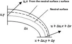
[image:2.595.229.379.326.418.2]

Because one side of inclusion thin-wall is air, it is almost considered as the prerequisite of only tangential normal stress. If we assume that thin-wall curve is smooth and its slope is not that steep, we can adopt the shell model of Kirchhoff-Love. This model equals to an arch that meets plane’s assumption in the case of strain plane, and only has positive strain along with the direction of tangent (shown in Figure 2). The normal commercial software does never fulfill this plane strain unit [9]. In order to make programming convenient, this article will make inferences of its corresponding expression under rectangular coordinate system，and then achieve element stiffness matrix.

Figure 2, microelement of the inclusion

We can know easily from microelement shown in Figure 2 that the original distance of tangential section away from z point to neutral surface is:

0 0

(1

0

)

l

= ∆

s

+

κ

z

(1)

0

κ

is the original curvature, expressed as follows:

0

y x

'' '

x y

'' '

κ

=

−

(2)

The derivative is differentiation of arc length. Pay attention to the requirements of Kirchhoff-Love that need

κ

₀

h

to be small. If thin-wall microelements have micro displacement

(

u s v s

( ), ( )

)

，the change of surface within thin

wall is

(

x s

( )

+

u s y s

( ), ( )

+

v s

( )

)

，each variable in formula (1) should be:

2 2

0 0

1 2 ' ' 2 ' '

'

'

(1

' '

' ')

s

s

u x

v y

u

v

s

u x

v y

∆ = ∆

+

+

+

+

= ∆

+

+

(3)

(

)(

) (

)

(

)

(

)

0

''

''

'

'

''

'' ( '

')

' ''

' ''

( ' ''

'' ')

s

y

v

x

u

x

u

y

v

s

x y

y x

x v

u y

κ

=

+

+

−

+

+

∆

∆

=

−

+

−

(

1

)

l

= ∆

s

κ

z

+

(5)

The above derivative uses the prerequisite that

(

∆ ∆ ∆ ∆

u

/

s

,

v

/

s

)

is a small value.

Therefore, the positive strain of each point with the direction of tangentiality can be presented as:

(

) (

)

(

) (

)

(

)

0 0 0

0

0 0

0

' '

' '

' ''

'' '

' '

' '

s

s

z

s

s

l l

l

s

u x

y v

z x v

u y

z

u x

y v

κ

κ

ε

κ

∆ − ∆ + ∆ − ∆

−

=

=

∆

=

+

+

−

+

+

(6)

Obviously, the first term in formula (6) stands for tensile strain mode similar to pole. The second term stands for curving strain mode similar to girder. The third term describes that fact that the bend of thin wall will absolutely lead to the curving strain simultaneously while stretching. And we can realize that when the neutral surface of thin wall is straight line, the strain mode expressed in formula (6) will degrade completely to be the combination of pole and girder.

The above formulae has second derivative of displacement

(

u s v s

( ), ( )

)

. While using finite element discretization, shape function should be second derivative. In order to make bending moment conveyed, the first derivative of connection point should be continuous. Therefore, the paper adopts the classic beam element of shape function called ‘two nodes and four parameters’ to insert value, that is:

( ) ( )

(

)

(

)

( )

2 3 2 3 2 3 3 2

1 3

2

2

'

'

'

'

,

3

2

'

'

'

'

T

i i i i

i i T i i

j j j j

j j j j

u

v

u

v

s

u

v

u

v

u

v

N

u

v

u

v

u

v

u

v

s

ξ

ξ

ξ

ξ

ξ

ξ

ξ

ξ

ξ

ξ

ξ ξ



₋

₊



_

_

_

_



_{ }

_

_

_

∆

−

+



_{ }

_

_

_





₌

_

_

₌





₋

_

_

_

_



_{ }

_

_

_



_∆

₋

_{ }

_

_

_













(7)

To especially point out that the term that is degree of freedom of junction angle

(

u v

', '

)

is the arc length’s derivative of translational movement without corresponding physical angle. The angle of linear neutral plane can be expressed as:

θ

= ⋅

(

n u

'

)

, and the strain field can be expressed as:

( )

[

]

[

]

2 2 2 ₂ 2

1

', '

', '

T T e e T T e e

d

d

d

d

z

z

x y

y x

s

_d

s

_d

d

_d

ξ

ξ

κ

ε ξ

ξ

ξ

















 

 

+









=

_

_

 

+

−

_

_

 

∆

 

∆

_

_

 





















N

N

u

u

v

v

N

N

(8)

In brief: ：

ε ξ

( )

( )

ξ

 

=

 

 

e e

u

B

v

, thereby the potential energy function and element stiffness within units are able to

be calculated as follows:

1 2 0 2

,

h e

T T T

h e e

e

s

J

dzd

ξ

−

 





Φ = ∆

_

_

 

 

∫ ∫

u v

B EB

u

v

(9)

and so element stiffness matrix can be gained as:

1 2 0 2 h T h

e

= ∆

s

∫ ∫

₋

J

dzd

ξ

K

B EB

(10)

3. The assembling of inclusion and matrix

degrees of freedom of inclusions and degrees of freedom of matrixes. The infliction of this constrainable relationship can refer to [11].

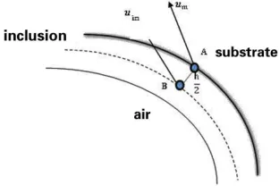
[image:4.595.224.380.138.246.2]

For each junction A of corresponding matrixes on interface, set junction B on neutral surface of inclusion in order to make the normal direction of AB along with curve on neutral surface seem like Figure 3.

Figure 3, interfacial points assignment

According to continuous model of interfacial displacement, AB is always perpendicular to neutral surface and has the fixed length no matter before or after transformation.

n

= −

(

y x

', ' ,

)

τ

=

(

x y

', '

)

_{, respectively is unit normal}

vector of inclusionary neutral surface and unit tangential vector before transformation:

2

m in

h

−

=

x

x

n

(11)

After transformation:

(

) (

)

(

)

(

)

0 0

0 0

,

2

'

2

m m in in

ds

ds

h

dy

dv

dx

du

ds

ds

ds

ds

h

+

−

+



₊

₊



=



−







=

−

⋅

x

u

x

u

n

u n

τ

(12)

get the difference between these two formula:

(

'

)

2

m in

h

−

= −

⋅

u

u

u n

τ

(13)

The above multi-points constraint makes the displacement on interfacial junction between matrix and inclusion equal. In order to these two fit better on the interface, we can add constrain conditions that tangent equals between inclusion and matrix. And, usually, plane unit junctions in commercial software does not have degrees of freedom of angle [10], matrix’s tangent on interfacial points can be calculated in accordance with isoperimetric element interpolation. Assume that the side of unit matrix on interface corresponds to the side of isoperimetric quadrilateral

1

η = −

:

(

)

(

)

(

1 1

)

//

|

,

|

m ξ η ξ η

v

τ

N

=−

x u N

+

=−

y

+

(14)

The tangent of interfacial junctions between these two units is calculated by weighted average of results gained from these two units. The weight in weighted average can be considered like that: before transformation, the tangent of matrix and inclusion on interface equals:

(

β

τ

0, 1m

+

α

τ

0, 2m

)

×

τ

0,in

=

0

(15)

(

β

τ

m1

+

α

τ

m2

)

×

τ

in

=

0

(16) To fulfill conveniently, this article uses multi-points constraint (13) to press conditions of border of interface.

4. Examples

For given foam with certain type included large a mount of compound materials distributing randomly in the matrix, its macroscopical attribute is determined by volume fraction of bubble and thickness of inclusion wall. By adjusting these two parameters, it is flexible to customize physical attributes of composite materials [19][20]. If we ignore the interacting influences of inclusions, we can establish a reference same as bubble’s volume fraction of macroscopical composite materials and thickness of wall. And then through the analysis we can estimate effective modulus of macroscopical composite materials [8].

In order to assure the correctness of this model, we first calculate the volume fraction of various inclusions and effective modulus under various thickness of wall, and then contrast it with traditional model. The traditional model uses Ansys 10.0 and PLANE42 as unit; so this article still uses Ansys basically as the model and then educes stiffness. And also the inclusion assembles and connects stiffness in the way that Section 2 and 3 perform, and then uses optimizer called HSL-MA57 to calculate.

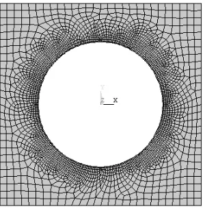
[image:5.595.233.378.349.498.2]

Example 1: as indicated in Figure 4, the size of section of compound materials is

100 100

×

, including round vacuoles with volume ratio equaling

µ

. The thickness of inclusion wall is h. The Young modulus of matrix materials and inclusion materials are respectively 1Mpa and 150Mpa, and Poisson’s ratios are respectively 0.4 and 0.3.

Figure 4，meshing plan of the proposed model (

µ =

0.3,

h

=

1

)

As the contrast of this article’s case, using Ansys traditional programs needs to adopt a more dense mesh to properly express inclusion of deformation. As indicated in Figure 5:

Figure 5，meshing plan of the solid model (

µ =

0.3,

h

=

1

)

[image:5.595.233.383.570.724.2]

modulus of composite materials can also be achieved. Under this condition, the modulus should be:

(

2

)

1

E

ν σ

ε

−

=

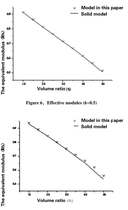
(17)

[image:6.595.199.422.157.522.2]

The result that achieved from equivalent modulus with the change of cavity volume fraction is shown in the following figure:

[image:6.595.199.399.168.325.2]

Figure 6，Effective modules (h=0.5)

Figure 7，Effective modules (h=1.0)

From Figure 6 and Figure 7, we can see that both of these two calculating results are very close. It matches the expectation that the equivalent modulus increases while the thickness of inclusions increases and the equivalent modulus decreases while volume fraction of vacuole increases. From the figure we can also find that the results of the two models fit better when mixed thickness is small, which also matches the assumption of Kirchhoff-Love’s thin-wall theorem. Therefore, the calculation scheme this paper proposes is valid.

We can also find that, under comparatively larger volume ratio of cavum, the result of equivalent modulus this paper calculates is a little bit larger than result plane unit calculates. There are three reasons: first, the gridding of Ansys entitative model is kind of thin; Second, thin-wall model ignores transformation in the direction of thickness; Third, connection of multi-points constraints has stiff effect on interface. And we know that the phenomenon is more obvious under bigger volume ratio of cavum through analysis, which also matches the analyses of Figure 6 and Figure 7.

[image:7.595.250.350.77.170.2]

Figure 8, debonding while under uniaxial stretch

Example 2: The former example uses

µ =

20%,

h

=

0.5

and two cases to calculate different equivalent modules under different size of destroyed interface.

The result is shown in Figure 9:

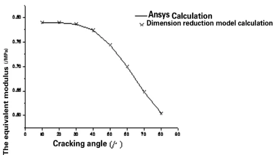
Figure 9, effective modules versus debonding angles

We can see that these two results are extremely close to each other, both showing that the value of equivalent modulus decreases suddenly when its dehiscent angle reaches a certain point (about 40 degree)； this phenomenon

shows that this kind of composite foam is probable to lose stableness because of the partial drop of interface while stretching, which matches the results of references [16][18]. The model this paper describes can be applied to the intimation of drop-off procedure of interface.

CONCLUSION

This paper tries to use combination of shell model on the basis of thin-wall theorem and practical model to solve plate problem of syntactic foams. Adopting shell model, in order to avoid the problem that the shell wall is too thin, the paper adopts very tiny gridding while establishing the model. The advantages of this approach are few degrees of freedom and low cost. The article uses the format of Kirchhoff-Love’s shell model in plane strain, and infers strain expression and stiffness matrix of inclusion, which makes programming easier by using whole rectangular coordinate system; And the article uses continuous displacement model of inclusion and matrix on interface, gaining the connecting constrainable relationship between plate shell and entity points, which was pressed by direct method; Take advantage of the above approach to research equivalent model of syntactic foams while the volume ratio and thickness of shell wall are changing; Simulate condition of partial drop-off on interface. Examples indicate that the calculating results of this paper and the traditional way are very close to each other, which proves to be effective.

In addition, we can find that thinner the thickness of wall is, so bigger the volume fraction of vacuole is, larger the modulus ration of inclusion and matrix is, and closer the two calculation results of these two models. And this is precisely the most common configuration parameter [1][2][3][6] in practical application, so this paper can be applied to statics calculations of composite foam and simulation of quasi-static degumming process.

REFERENCES

[image:7.595.171.443.252.405.2]

[3]Gupta N, Kishore, Woldesenbet E, Sankaran S. Journal of Materials Science, 2001, 36(18):4485–4491. [4]Rohatgi PK, Gupta N, Alaraj S. Journal of Composite Materials, 2006, 40 (13):1163–1174.

[5]Gupta N, Woldesenbet E. Composite Structures, 2003, 61(4):311–320. [6]Lu Zixing. Advances in mechanics 2004 , 34 (3) : 341 - 348.

[7]Bardella L , Genna F. Inter. J. Solids and Struct , 2001 , 38 (40-41) :7235- 7260.

[8]Tagliavia G, Porfiri M, Gupta N. International Journal of Solids and Structures, 2010, 47(16):2164-2177. [9]Carrera E. Archives of Computational Methods in Engineering, 2002, 9:87–140.

[10]Ansys Inc. Release 10.0 Documentation for Ansys[M/EB]. 2005:Chapter 4. [11]Felippa CA. Introduction to finite element method [EB/OL].

http://www.colorado.edu/engineering/cas/courses.d/IFEM.d, [2011-10-25]: Ch.08- Ch.09 [12]Jasiuk I, Tsuchida E, Mura T . Int J Solids Struct, 1987, 23 (10) : 1373- 1385. [13]Hashin Z. J App l Mech, 1991, 58 (2): 444- 449.

[14]Zhong Z, Meguid S A. J Appl Mech, 1999, 66 (4) : 839-846.

[15]Shen H, Schiavone P, Ru CQ, et al. Math Mech Solids, 2000, 5 (4) : 501- 510. [16]Needleman A. ASME J Appl Mech, 1987, 54 ( 3) :525- 553.

[17]Huang ZP, Wang J. Acta Mechanica, 2006, 182:195-210

[18]Tan H, Liu C. Journal of the Mechanics and Physics of Solids, 2005, 53: 1892-1917 [19]Gupta N, Ricci W. Materials Science and Engineering A. 2006, 427(1-2):331–342.