An image classification algorithm using fuzzy support vector machine

Journal of Chemical and Pharmaceutical Research, 2014, 6(5):1854-1861

Research Article

_{CODEN(USA) : JCPRC5}

ISSN : 0975-7384

An image classification algorithm using fuzzy support vector machine

Cao Jianfang

1,2

,

Chen Junjie

2

and Chen Lichao

3

1_{Department of Computer Science & Technology, Xinzhou Teachers University, Xinzhou City, China} 2_{College of Computer & Software, Taiyuan University of Technology, Taiyuan City, China}

3_{College of Computer Science & Technology, Taiyuan University of Science and Technology, Taiyuan City, China}

_____________________________________________________________________________________________

ABSTRACT

The development of electronic technology and imaging technology has resulted in the rapid growth of digital images. It has become an urgent problem to rely on advanced technology to identify images. An image recognition algorithm based on fuzzy support vector machine is proposed. The algorithm makes up for the lack of traditional support vector machine in multi-classification problems and solves the problem of semantic ambiguity in image classification by defining fuzzy membership function. Using 6 types of natural images to test, the experimental results show that classification performance improves significantly compared with the traditional support vector machine method.

Key words: fuzzy support vector machine, fuzzy membership function, features extraction, image semantics, image

classification

_____________________________________________________________________________________________

INTRODUCTION

With the development of electronic technology and the Internet technology, and the rapid popularization of image acquisition devices such as digital cameras, camera device and electronic camera etc. in recent years, the digital image has a rapid expansion of the scale and there will be GB even TB of digital images to be generated, published and shared every day. Images play a very important role in people's life. People can perceive rich information containing in the image when they observe an image: the target, the spatial layout, function and scene semantic, even the emotion semantic image brings to people [1, 2]. However, the massive image data brings people not only convenience, but also a lot of problems: People are difficult to find the information of their real needs in the voluminous data and information. Faced with such a large-scale image resources, how to make the organization and classification effectively for them has become an urgent problem to be solved at present.

Currently, there are many algorithms to be used for image classification, such as the Bayes classifier, K-nearest neighbor classification, neural network, genetic algorithm, clustering etc. But only under the condition of adequate samples, can the performance of these classification methods have the theoretical guarantee, and in fact, the number of samples is often limited. Therefore the classification effect of the above algorithms in practical application is not just as one wish.

This paper is organised as follows. In Section 2 we first discuss the fuzzy support vector machine algorithm. Then, in Section 3, we propose an algorithm for image classification based on fuzzy support vector machine in detail. Then, experimental results are presented in Section 4. Finally, Section 5 presents our conclusions and future work.

II. FUZZY SUPPORT VECTOR MACHINE

A. Standard support vector machine

The core idea of the standard support vector machine is to create a low VC dimension optimal classification hyperplane in high dimensional kernel space by putting learning samples mapping into a high dimensional kernel space nonlinear. The classification function of which the upper bound of risk is minimized is obtained, considering the size of experience risk and confidence interval, according to the principle of structural risk minimization for its eclectic.

Supposing separable sample set is

(

x

i

,

y

i

),

i

=

1

,

L

,

n

,

x

∈

R

n

,

y

∈

{

+

1

,

−

1

}

, the main purpose of SVM is to

construct a hyperplane to split the two kinds of different samples, which makes the classification interval maximum. Thus we have the following quadratic optimization problem:

2

1

1

min(

)

2

n

i i

C

ω

ε

=

+

∑

s. .

t y

_i

[

ω

x

_i

+ − + ≥

b

] 1

ε

_i

0

(1)

i

0

ε

≥

Introducing Lagrange multipliers, we get its dual form:

1 , 1

1

max

( ,

)

2

n n

i i j i j i j

i i j

y y K x x

α

α α

= =

−

∑

∑

s. .

t

0

≤

α

i

≤

C

(2)

1

0

n

i i i

y

α

=

=

∑

Among them,

ε

_i is the slack variables, C is the penalty coefficient,

K x x

( ,

i j

)

is the kernel function. Thus the

decision function is:

1

( )

(

( , )

)

n

i i i

i

f x

sign

α

y K x x

b

=

=

_∑

+

(3)

B. Multi-class support vector machine

SVM applied to multi-class classification problem can be roughly divided into two categories [3].

(1) One-to-one. The method is to train a SVM classifier in each of the two classes of samples, which can obtain

k(k-1) /2 classifiers, and the number of classifier associated with each category is k-1. When predicting the unknown

sample, each classifier judges its category and the corresponding category wins a vote. The category of unknown sample is the final category having the most votes.

(2) One-to-many. The method is to use a SVM classifier to distinguish each class separately from other types of class, resulting in the k classifiers. When predicting the unknown sample, the sample is classified in that category with the greatest decision function values.

For the above two methods, when the number of classes is more, training speed and classification speed is slower and they have no-identifiable areas. Then there are several improved algorithm, including ECOC, DAG etc. For ECOC method, it’s different to select appropriate samples; For DAG method, its shortcomings are: (i) When the category number for the classification is much, the training speed is low; (ii) the selection of root node may directly affect the result of classification.

C. Fuzzy support vector machine

(1) Introduction of fuzzy support vector machine

different contributions when the objective function is constructed. And samples with noise or wild values get less weight so as to achieve the purpose of eliminating noise and affection of outliers in the sample [10].

When using fuzzy support vector machine for classification, it’s different from the conventional SVM for the representation of the training sample that fuzzy support vector machine adds membership in addition to the characteristics of the sample and generic identification. Supposing the training sample set is expressed as:

( ,

x y

_{i i}

, ( )),

µ

x

_i

i

=

1, 2,

_L

, ,

n x

∈

R

n

,

y

∈ + −

{ 1, 1}

Among them,

µ

( )

x

_i is a membership,

0

p

µ

( ) 1

x

_i

≤

. Since the membership

µ

( )

x

_i indicates the degree that the sample belongs to a certain class and

ε

_i is classification error term in the objective function of SVM,

µ

( )

x

_i

ε

_i is the error term with the weight, and the optimal classification plane we get is the the optimal solution of the following objective function:













+

∑

=

n

i

i i

x

C

w

1 2

)

(

2

1

min

µ

ε

s.t.

y

_i

[

wx

_i

+

b

]

−

1

+

ε

_i

≥

0

(4)

ε

_i

≥

0

Adding Lagrange multipliers

α

_i

(

i

=

1, 2,

L

, )

n

, we get its dual form:

∑

∑

= =

−

n

j i

j i j i i i n

i

i

y

y

K

x

x

1 , 1

)

,

(

2

1

max

α

α

α

s.t.

0

≤

α

_i

≤

C

µ

(

x

_i

)

(5)

0

1

=

∑

=

n

i i i

y

α

The decision function is:













+

=

∑

=

n

i

i i

i

y

K

x

x

b

sign

x

f

1

)

,

(

)

(

α

(6)

By comparing the formula (5) with (2), we can see that fuzzy support vector machine (FSVM) is different from support vector machine (SVM) on the constraint conditions. The parameter C in SVM is a custom penalty factor and controls the degree of punishment for wrong classified samples. The larger C is, the greater the punishment is and the degree of constraint for wrong classified samples, the smaller the interval of the classification is. With the loss of

C, support vector machine algorithm would ignore more samples and get a classification surface with a larger edge

interval. For fuzzy support vector machine, if we set the value of C larger and take the membership degree

( )

x

i

µ

with 1, fuzzy support vector machine degrades general support vector machine, which allows smaller classification error rate and gets classification surface with narrower edge. The fuzzy support vector machine algorithm can reach the effect of different degree of punishment with different samples through giving different membership degree for different samples. The smaller the membership degree is, the smaller role in training sample is. As a result, the fuzzy support vector machine has stronger anti-interference ability than support vector machine.

(2) The determination of fuzzy membership degree

This paper will use the measure method of fuzzy membership degree to determine the fuzzy membership

µ

( )

x

i . It regards the membership as a function of the distance between the samples in feature space and its class center. Let

0

x

be the class center, r be class radius, r is determined by the following formula.

o i i

x

x

r

=

_max

−

(7)

Then the membership of each sample is:

δ

µ

=

−

−

+

r

x

x

x

_i

)

1

i o

(

(8)

Wherein,

δ

is a small preset constant (

δ

>

0

) to avoid the situation

µ

( )

x

_i

=

0

.

III.IMAGE CLASSIFICATION USING FUZZY SUPPORT VECTOR MACHINE

A. The general process of image classification

The general process of image classification is: image capture, image preprocessing, image feature extraction, classifier decision, etc. The classification process is as follows in figure 1.

B. Image preprocessing

Because the actual image data are always incomplete, have noises and are inconsistent, preprocessing becomes more and more important. There are two kinds of data preprocessing technique for data mining of image data [4-5]: data cleaning and data transformation. The first step of image preprocessing is to use the denoising technology to process images. The denoising of images may remove most of the background information and noise. Classification effect also depends on the features extracted from the image to a large extent. The second step is image enhancement in image preprocessing. In the process of image generation, transmission or transformation, image quality always reduces due to the influence of various factors. The purpose of image enhancement is to adopt a series of technology to improve the effect of the image or transform the image into a more suitable form for processing. We can use the widespreadly used histogram equalization technology to realize the image enhancement.

C. Feature Extraction

Feature extraction is a crucial step in the process of image classification. The quality of feature extraction will directly affect the performance of the classifier [6-8]. This paper uses three kinds of characteristics (color, texture, edge direction) to express image content for an image.

(1) Color feature

The colors of image carry a wealth of semantic information; color feature is most commonly used visual features in image classification. RGB color, being composed of R, G, B components, is the most common color space. Now a variety of images use RGB space to store and transport, and RGB color gets direct support of various physical devices. However, the studies find that the RGB components are not independent of each other, and exist some correlation. But HSV color space has a better independence property of visual perception, and it can feel continuously change from all kinds of color components. In the other word, the color change that the human eye can perceive can be measured by the Euclidean distance of the color components. Therefore this paper adopts HSV color space. Calculation process is as follows: given color point (r, g, b) of the RGB color space, the color point (h, s, v) of the HSV color space is：

Assume:

v

'

=

max( , , )

r g b

， define：

r

'

，

g

'

，

b

'

=

∑∑

G

i G

j

d

j

i

P

ENG

2

(

,

|

,

θ

)

Figure 1. The process of image classification

original images

image

[

]

∑∑

= =

−

+

=

G i G j

j

i

d

j

i

P

IDM

1 1 2

)

(

1

/

)

,

|

,

(

θ





















−

=

=

+

≠

=

−

=

=

+

≠

=

−

=

=

+

=

otherwise

r

b

g

r

r

b

g

r

b

if

g

b

g

r

b

b

g

r

g

if

b

b

g

r

b

b

g

r

g

if

r

b

g

r

g

b

g

r

r

if

g

b

g

r

g

b

g

r

r

if

b

h

　

，

　

　

，

　

　

，

　

　

，

　

　

，

　

　

'

5

)

,

,

min(

)

,

,

max(

'

3

)

,

,

min(

)

,

,

max(

'

3

)

,

,

min(

)

,

,

max(

'

1

)

,

,

min(

)

,

,

max(

'

1

)

,

,

min(

)

,

,

max(

'

5

'

min(

,

,

)

'

b

g

r

v

r

v

r

−

−

=

)

,

,

min(

'

b

g

r

v

g

v

g

−

−

=

(9)

)

,

,

min(

'

b

g

r

v

b

v

b

−

−

=

255

'

)

,

,

min(

'

60

v

v

v

b

g

r

v

s

h

h

=

×

　

=

−

　

=

Among them,

, ,

[0, 255]

[0, 360]

r g b

∈

，

h

∈

,

s

∈

[0,1]

,

s

∈

[0,1]

.

For HSV color space, the distance between

c

₁

=

( , , )

h s v

_{1 1 1} and

c

₂

=

( ,

h s v

_{2 2}

,

₂

)

can be calculated using the following formula:

[

2 2

1 2 1 2 1 1 2 2

( ,

)

(

)

( cosh

cosh )

d c c

=

v

−

v

+

s

−

s

+

( sinh

s

_{1 1}

−

s

₂

sinh )

₂ 2



_

1/2 (10) The similarity between two colors is:

1 2 1 2

1

( ,

)

1

( ,

)

5

s c c

= −

d c c

(11)

(2) Texture feature

Texture reflects local structure feature of the image, specifically say, it is change of the pixel grayscale or color in the image of a pixel neighborhood. The change is related in the spatial statistics, which consists of texton and arrangement of primitive. This paper proposes texture feature extraction method based on proposed GLCM combining the definition of texture. GLCM reflects comprehensive information of image gray on direction, interval and magnitude of changes based on second-order joint conditional probability density function between image gray degrees [11,12]. Supposing

P i j d

( , | , )

θ

is the probability of occurrence of each pixel having a gray level i and j giving space distance d and direction

θ

, which is usually expressed in matrix form, called GLCM. If the gray level of an image is G, the co-occurrence matrix is a G×G square matrix. Image texture features can be described by calculating secondary statistic of GLCM. This method defines 14 texture features, only four of which are not relevant: energy, homogeneity, contrast and correlation. The computing methods are as follows.

Energy: (12) Homogeneity: (13) Contrast: (14)

∑∑

=

G i G j

d

j

i

P

ENG

2

(

,

|

,

θ

)

Correlation:

(15)

∑

∑

= =

=

G

j G

i

d

j

i

P

i

1 1

1

(

,

|

,

θ

)

µ

∑

∑

= =

=

G

i G

j

d

j

i

P

j

1 1

2

(

,

|

,

θ

)

µ

∑

∑

= =

−

=

G

i

G

j

d

j

i

P

i

1 1

2 1 2

1

(

µ

)

(

,

|

,

θ

)

σ

∑

∑

= =

−

=

G

j

G

i

d

j

i

P

j

1 1

2 2 2

2

(

µ

)

(

,

|

,

θ

)

σ

Energy is local homogeneity measure of images. For the homogeneous regions, the particular pixel pairs are more and few element values of GLCM are larger, which result in that the energy values are larger. Homogeneity reflects the degree of texture thickness and gray uniformity, high-value array elements which concentrate near the main diagonal and the values are larger. Contrast measures the amount of local change and reflects the degree of the

groove depth of the texture. In formula (14),

i

−

j

indicates gray-scale difference of the pixel pairs. The more the pixel pairs with large gray-scale difference are, the greater the contrast value is. Correlation measures the degree of similarity of GLCM elements in direction of row or column and reflects the correlation between pixel gray values of images.

(3) Edge feature

Edge feature is the most basic characteristics because the edge includes the boundary information of valuable target which can be used for image analysis, image filtering, and object recognition. Canny operator is used to test the edge in this paper and we can get a binary image retaining only the edge, and then calculate the following characteristics for the edge image.

(i) Edge length. That is the number of the non-zero pixels in the image. The value indicates the total length of the inner edge of the image.

(ii) Minkowski dimension, namely Minkowski fractal dimension of edge. This feature can effectively describe the extent of the sparse of image edges. Calculation of the fractal dimension needs use a series of structural elements of different sizes to expand the edge image. With the increase of the size of the structural elements, the total number of non-zero pixes (edge points) is also increasing. The more intensive image edge is, the faster speed of the increasing of total number N of edge points with the enlargement of size S of structure element is. We make linear fitting for logarithm of N and S, and get the slope G of the fitted line. The fractal dimension of the image is defined D=2-G.

D. Classification method

According to the classification process shown in the above figure 1, input the original image, the first step is to make pretreatments, such as noise reduction, enhancement etc. This step has the ability of reducing speckle noise in flat areas and keeps details with obvious changes. Then, extract color, texture and edge features. RGB color space is converted into HSV color space when extracting color feature. Texture features includes energy, homogeneity, contrast and correlation. Edge feature includes edge length and Minkowski dimension. Finally, the extracted feature vector is input to the FSVM classifier and we can obtain classification results.

RESULTSANDDISCUSSION

Experimental data come from ordinary natural images from Internet. These images are divided into six classes: architecture, animal, landscape, plant, people, interior decorating. We use support vector machine and fuzzy support vector machine for classification respectively. Sample images used in the experiment are shown in Table 1.

TABLE 1: IMAGE SAMPLES USED IN THE EXPERIMENT

sample classification architecture animal landscape plant people interior decorating

Train sample 200 200 160 180 160 120

Test sample 170 180 160 150 150 100

The number of unclassified samples USS: the number of samples in test set being not classified (ie. The sample is neither properly classified nor misclassified).

Unclassified rate USR: the proportion of unclassified samples in total samples in the test set.

t

USS

USR

N

=

(16)

t

N

is total number of samples in test set.

The number of classified samples CSS: the number of samples which are not properly classified by SVM, but are properly classified by FSVM.

Classified sample rate CSR: the proportion of classified samples in unclassified samples.

CSS

CSR

USS

=

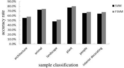
(17)

[image:7.595.178.413.280.410.2]

The classification results of the two methods are shown in Figure 2 and Table 2.

TABLE 2 : COMPARISON OF CLASSIFICATION PERFORMANCE BETWEEN SVM AND FSVM

sample classification the number of test samples USS USR CSS CSR

architecture 170 8 4.3% 4 52.0%

animal 180 12 7.1% 5 42.1%

landscape 160 5 2.9% 0 0.0%

plant 150 7 5.0% 3 43.4%

people 150 4 2.8% 0 0.0%

interior decorating 100 6 6.2% 2 34.1%

We can clearly see from the above experimental data that classification performance of fuzzy support vector machine is superior to that of support vector machine. The degree of superior depends on the number of not classified samples. The more the number of not classified samples, the better the performance of fuzzy support vector machine is. If not having not classified samples, fuzzy support vector machine has the same performance as support vector machine.

CONCLUSION

This paper uses fuzzy support vector machine to make the classification research on natural images. Aiming at the problem of no-identifiable areas existing in the support vector machine when dealing with multi-class classification problem, we introduce fuzzy membership function to solve the problem. In order to evaluate the effect and performance of classification methods, we have done experiments using different types of image. The experimental results show that image classification method based on fuzzy support vector machine is superior to that based on support vector machine.

ACKNOWLEDGMENT

This work was supported by National Natural Science Foundation of China under Grant No. 61202163 and by the Natural Science Foundation of Shanxi Province under Grant No.2012011011-5 and No. 2013011017-2 and by the Technology Innovation Project of Shanxi Province under Grant No. 2013150 and by the Key disciplines supported

sample classification

ac

cu

ra

cy

r

at

e

by Xinzhou Teachers University under Grant No. XK201308. The authors are grateful for the constructive and valuable comments made by the many expert reviewers.

REFERENCES

[1]Jen sen J R. Introductory Digital Image Processing: A Remote Sensing Perspective. Third Edition. Beijing:

China Machine Press, 2007.

[2]J. Li, Allison N M. Neurocomputing, vol.71, no. 10-12, 2008, pp.1771-1787. [3]W. Ying, Z. G. Wang, J. L. An. Computer Engineering, no.16, 2006, pp. 74-76.

[4]Marin F, Nozha B. IEEE Transactions on Geoscience and Remote Sensing, vol. 45, no.4, 2007, pp. 818-826. [5]X. Sun, Y. D. Xie, D. C. Ren, Computer Engineering and Design, vol. 31, no. 21, 2010, pp.4653-4654. [6]G. Y. Wang, J. F. Kang. Computer Engineering and Design, vol. 32, no. 1, 2011, pp. 236-239.

[7]Rachel LO T W, Paul Siebert J. Computer Vision and Image Understanding, vol. 113, no. 12, 2009, pp. 1235-1250.

[8]Chow T W S, Rahman M K M． Neurocomputing, vol. 70, no. 4-6, 2007, pp. 1040-1050．

[9]Hall M, Frank E, Holmes G, et al. The WEKA data mining software: an update// Sigkdd Explorations. New York,

NY, USA: ACM, 2009, pp.10-18．

[10]TOMMASI T, ORABONA F, CAPUTO B. An SVM confidence-based approach to medical image annotation // Proc of Cross-Language Evaluation Forum. Berlin: Springer-Verlag, 2008, pp.696-703．