Fight or Flight?

Munich Personal RePEc Archive

Fight or Flight?

Deck, Cary and Sheremeta, Roman

2012

Online at

https://mpra.ub.uni-muenchen.de/52130/

Fight or Flight? Defending Against Sequential

Attacks in the Game of Siege

*

Cary Deck

_{and Roman M. Sheremeta}

a _{Department of Economics, University of Arkansas}

Fayetteville, AR 72701, USA

phone: +1-147-575-6226, fax: +1-479-575-3241 email: cdeck@walton.uark.edu

and Economic Science Institute, Chapman University

b _{Argyros School of Business and Economics, Chapman University,}

One University Drive, Orange, CA 92866, USA

November 8, 2011

Abstract

This paper examines theory and behavior in a two-player game of siege, sequential attack and defense. The attacker’s objective is to successfully win at least one battle while the defender’s objective is to win every battle. Theoretically, the defender either folds immediately or, if his valuation is sufficiently high and the number of battles is sufficiently small, then he has a constant incentive to fight in each battle. Attackers respond to defense with diminishing assaults over time. Consistent with theoretical predictions, our experimental results indicate that the probability of successful defense increases in the defenders valuation and it decreases in the overall number of battles in the contest. However, the defender engages in the contest significantly more often than predicted and the aggregate expenditures by both parties exceed predicted levels. Moreover, both defenders and attackers actually increase the intensity of the fight as they approach the end of the contest.

Keywords: Colonel Blotto, conflict resolution, weakest-link, game of siege, multi-period resource allocation, experiments.

Word Count: 8554

Acknowledgments: We thank Subhasish M. Chowdhury, Amy Farmer, Kjell Hausken, Dan Kovenock, Brian Roberson, Steven Tucker, and seminar participants at Chapman University for helpful comments. We also gratefully acknowledge comments from an associate editor and two anonymous referees. We retain responsibility for any errors. The data analyzed in this paper are

1. Introduction

Environments, such as cyber-security (Moore et al., 2009), pipeline systems (Hirshleifer,

1983), complex production processes (Kremer, 1993), and anti-terrorism defense (Sandler and

Enders, 2004) can be characterized as weakest-link systems. In each of these cases an attacker

only needs to disrupt one component of the system to create a total failure. Defenders are forced

to constantly protect the entire system while attackers are encouraged to seek the weakest point.

Recently, a number of theoretical papers emerged trying to model the optimal strategies

of those who wish to protect weakest-link systems and those who wish to destroy them. Most of

the theoretical work has been focused on the case where the attacker and the defender

simultaneously decide how much to invest in each potential target, a variation of the Colonel

Blotto game.1 For example, Clark and Konrad (2007) and Kovenock and Roberson (2010) both

provide a theoretical analysis of a multi-battle two-player game where the attacker and the

defender simultaneously commit resources to concurrent multiple battles in order to win a prize.2

To receive the prize, the attacker needs to win at least one battle, while the defender must win all

battles. Another class of attack and defense games, distinct from the simultaneous multi-battle

game, assumes that battles proceed sequentially. Most of such models originated with the

seminal R&D paper of Fudenberg et al. (1983).3 _{The theoretical model studied in our paper,}

however, is most closely related to Levitin and Hausken (2010). Both papers consider a contest

in which a defender seeks to protect a network and an attacker seeks to destroy it through

multiple sequential attacks.4 Levitin and Hausken (2010) model the probability of winning a

given battle with a lottery contest success function. Due to complexity of their model, most of

the paper’s theoretical results are based on numerical simulations. In contrast, our paper uses an

theoretically. We also conduct a series of controlled laboratory experiments and compare

observed behavior to the theoretical benchmarks.

Sequential attacks in a weakest-link network can be viewed as a “game of siege” where

the defender attempts to hold an asset such as a fort or a landing strip against repeated assault.

Arguably, the most famous siege, whether it is true or not, was the battle of Troy in which the

Greeks finally ended a prolonged siege by hiding in a wooden horse according to Greek

mythology. In this type of game, the attacker and defender decide how much to invest in each

battle after learning the outcome of any previous battle. The side making the larger investment

wins that battle, creating a series of all-pay auctions. The attacker only needs to be successful

once, while the defender must repel each successive assault to win, and hence the game has a

weakest-link structure. Our theoretical model predicts that if the defender’s valuation is

sufficiently high and the number of battles is sufficiently small, then the defender has a constant

incentive to fight in each battle and otherwise he folds immediately. Thus, defenders exhibit a

response pattern of “fight or flight.” Attackers respond to defense with diminishing assaults over

time. Consistent with theoretical predictions, our experimental results indicate that the

probability of successful defense increases in the defender’s valuation and it decreases in the

overall number of battles in the contest. However, the defender engages in the contest

significantly more often than predicted and the aggregate expenditures by both parties exceed

predicted levels. Also, contrary to theoretical predictions, both the defender and attacker actually

increase the intensity of the fight as they approach the known end of the game.

Identifying the predictive success of contest models, such as the one described in the

current study, is of social value. However, the usual concerns about unobservable information

costly in this context, making laboratory experiments an ideal tool for empirical validation. Our

study adds to the experimental literature on multi-battle contests. To date there are only a few

experimental studies that investigate games of multiple contests. Avrahami and Kareev (2009)

and Chowdhury et al. (2011) test several basic predictions of the original Colonel Blotto game

and find support for the major theoretical predictions. Kovenock et al. (2010) study a

multi-battle contest with asymmetric objectives and find support for the theoretical model of Kovenock

and Roberson (2010) but not Clark and Konrad (2007). Our study contributes to this literature

by investigating both theoretically and experimentally the dynamic multi-battle contest which we

call the “game of siege.”

2. The Game of Siege

Before introducing the general model of sequential attack and defense (or game of siege),

it is useful to review the simple one shot contest, or all-pay auction, between two asymmetric

players as in Baye et al. (1996). Assume that two risk-neutral players compete for a prize in a

contest. The prize valuation for player 1 is 𝑣₁ and for player 2 it is 𝑣₂, where 𝑣₁ > 𝑣₂ > 0. Both

players expend resources 𝑥₁ and 𝑥₂, and the player with the highest expenditures wins. In case of

a tie, the winner is selected randomly. Irrespective of who wins the contest, both players forfeit

their expenditures. It is well known that there is no pure strategy equilibrium in such a game

(Hillman and Riley, 1989; Baye et al., 1996). The mixed strategy Nash equilibrium is

characterized by the following proposition due to Baye et al (1996).

Proposition 1. In the mixed strategy equilibrium of a contest between two asymmetric

(i) Players randomize over the interval 𝑥 ∈ [0, 𝑣₂], according to cumulative distribution

functions 𝐹₁∗(𝑥) =_𝑣𝑥

2 and 𝐹2

∗_{(𝑥) = 1 −}𝑣2

𝑣1+

𝑥 𝑣1.

(ii) Player 1’s expected expenditure is 𝐸(𝑥₁) =𝑣2

2 and player 2’s is 𝐸(𝑥2) = 𝑣₂2

2𝑣1.

(iii) Player 1’s expected payoff is 𝐸(𝜋₁) = 𝑣₁− 𝑣₂ and player 2’s is 𝐸(𝜋₂) = 0.

(iv) Player 1’s probability of winning is 𝑝₁ = 1 − 𝑣2

2𝑣1and player 2’s is 𝑝2 =

𝑣2

2𝑣1.

We now turn to the case of two players, attacker and defender, competing in multiple

sequential contests. The objective of the attacker 𝐴 is to win a single battle, in which case he

receives a valuation of 𝑣_𝐴. The objective of the defender 𝐷 is to win all 𝑛 battles, in which case

he receives a valuation of 𝑣_𝐷, where 𝑣_𝐷 > 𝑣_𝐴 > 0. As the battles occur sequentially, both players

first simultaneously allocate their respective resources 𝑥_𝐴1 and 𝑥_𝐷1 in battle 1. If 𝑥_𝐴1 > 𝑥_𝐷1, then the

contest stops and the attacker receives 𝑣_𝐴. However, if the defender is successful in battle 1, the

contest proceeds to battle 2. Again, if 𝑥_𝐴2 > 𝑥_𝐷2, then the contest stops and the attackers receives

𝑣𝐴. This process repeats until either the attacker wins one battle or the defender wins all 𝑛

battles. The net payoff of player 𝐴 if he wins is equal to the value of the prize minus the

expenditures spent during the competition in each battle up to that point, e.i. 𝜋_𝐴 = 𝑣_𝐴− ∑𝑙_𝑘=1𝑥_𝐴𝑘,

where l is the battle won by the attacker. If player 𝐴 is never successful, this payoff (loss) is the

negative sum of his expenditures, i.e. 𝜋_𝐴 = − ∑𝑛_𝑘=1𝑥_𝐴𝑘. The payoff to player 𝐷 is similar, i.e.

𝜋𝐷 = 𝑣𝐷− ∑𝑛𝑘=1𝑥𝐷𝑘 if player 𝐷 wins all the battles and 𝜋𝐷 = − ∑𝑙𝑘=1𝑥𝐷𝑘 if he loses battle l.

To analyze this game we apply backward induction and identify the subgame perfect

equilibrium. As will be shown, the expected contest winner depends on the size of 𝑛 for a given

𝑣𝐴 and 𝑣𝐷. Specifically, the expected outcome depends on whether 𝑣𝐷 ≥ 𝑛𝑣𝐴, 𝑛𝑣𝐴 > 𝑣𝐷 > (𝑛 −

winning the contest for player 𝐷 is 𝑣_𝐷 and the value for player 𝐴 is 𝑣_𝐴, with 𝑣_𝐷 > 𝑣_𝐴. Therefore,

this is a simple one-stage contest between two asymmetric players as characterized by

Proposition 1. In such a contest, the expected expenditure of player 𝐷 in battle 𝑛 is 𝐸(𝑥_𝐷𝑛) =𝑣𝐴 2

and the expenditures of player 𝐴 is 𝐸(𝑥_𝐴𝑛) = 𝑣𝐴2

2𝑣𝐷. According to Proposition 1, the expected

payoff of player 𝐷 in battle 𝑛 is 𝐸(𝜋_𝐷𝑛) = 𝑣_𝐷− 𝑣_𝐴 and the expected payoff of player 𝐴

is 𝐸(𝜋_𝐴𝑛) = 0.

Next, we consider the contest in the penultimate battle. The defender’s continuation

value of winning battle 𝑛 − 1 is 𝑣_𝐷− 𝑣_𝐴 (his expected payoff from competing in battle 𝑛) and

his value of losing is 0 (since the contest stops if the attacker wins even a single battle). On the

other hand, the value to the attacker of winning battle 𝑛 − 1 is 𝑣_𝐴 (since the attacker only needs a

single victory) and the value of losing is 0 (the expected payoff from competing in battle 𝑛).

Given, these expected payoffs, the contest in battle 𝑛 − 1 is again a simple single stage contest

between two asymmetric players as characterized by Proposition 1. However, this time the

continuation value of player 𝐷 is 𝑣_𝐷− 𝑣_𝐴 and the value of player 𝐴 is 𝑣_𝐴. If the defender’s

continuation value is sufficiently higher than the attackers value, i.e. 𝑣_𝐷− 𝑣_𝐴 > 𝑣_𝐴, then the

defender has the advantage and his expected payoff in battle 𝑛 − 1 is 𝑣_𝐷 − 2𝑣_𝐴, while the

attacker’s expected payoff is 0.

A similar exercise can be performed for battle 𝑛 − 𝑘, the results of which are reported in

Panel A of Table 1. Note that in generating Panel A of Table 1, we assume that 𝑣_𝐷 ≥ 𝑛𝑣_𝐴 (or

alternatively that 𝑛 ≤𝑣𝐷

𝑣𝐴), i.e. the defender’s valuation is sufficiently high relative to the number

of battles 𝑛and attacker’s valuation 𝑣_𝐴. In such a case, the defender always randomizes between

the other hand, the expenditure of the attacker 𝐸(𝑥_𝐴𝑛−𝑘) = (𝑣𝐴)2

2(𝑣𝐷−𝑘𝑣𝐴) is decreasing in 𝑛 − 𝑘,

which means that the attacker’s aggression decreases in number of battles won by the defender.5

We summarize these findings in the following proposition:

Proposition 2. In the subgame perfect equilibrium, if 𝑣_𝐷 ≥ 𝑛𝑣_𝐴, then in battle 𝑛 − 𝑘:

(i) Player 𝐷 randomizes over the interval 𝑥_𝐷 ∈ [0, 𝑣_𝐴], according to the cumulative

distribution function 𝐹(𝑥_𝐷) =𝑥𝐷

𝑣𝐴, and player 𝐴 randomizes according to the cumulative

distribution function 𝐹(𝑥_𝐴) = 1 − 𝑣𝐴 𝑣𝐷−𝑘𝑣𝐴+

𝑥𝐴

𝑣𝐷−𝑘𝑣𝐴.

(ii) Player 𝐷’s expected expenditure is 𝐸(𝑥_𝐷𝑛−𝑘) = 𝑣𝐴

2 and player 𝐴’s expected expenditure is

𝐸(𝑥𝐴𝑛−𝑘) = (𝑣𝐴)

2

2(𝑣𝐷−𝑘𝑣𝐴).

Proposition 2 is based on the assumption that the defender has a relatively high

valuation.6 Now consider the case that 𝑛𝑣_𝐴 > 𝑣_𝐷 > (𝑛 − 1)𝑣_𝐴 (or alternatively that 𝑣𝐷

𝑣𝐴 < 𝑛 <

𝑣𝐷

𝑣𝐴+ 1). As shown in Panel B of Table 1, in this special case, the disadvantaged defender in

battle 1 receives expected payoff of zero. The attacker, on the other hand, receives positive

expected payoff of 𝑛𝑣_𝐴 − 𝑣_𝐷 and should attack. Although the defender does not entirely give up

in this case, his expected expenditures in battle 1 are lower than the expenditures of the attacker.

Should the defender win this initial battle, he would have the advantageous position in battle 2

and all subsequent battles and the game would progress as in Proposition 2.

If the player 𝐷’s valuation 𝑣_𝐷 is sufficiently small or the number of battles is sufficiently

high, then the defender will give up, by expending 0 resources in the first battle.7 _{To demonstrate}

this, assume that in battle 2 the continuation value of the defender 𝑣_𝐷− (𝑛 − 2)𝑣_𝐴 is not enough

(𝑛 − 1)𝑣𝐴 ≥ 𝑣𝐷 or 𝑛 ≥𝑣_𝑣𝐷_𝐴+ 1). In such a case, the attacker has an advantage in battle 2 over the

defender. According to Proposition 1, the expected payoff to the attacker is (𝑛 − 1)𝑣_𝐴− 𝑣_𝐷,

which for now assume is strictly positive, and the expected value to the defender is 0. Therefore,

when making a decision in battle 1, the defender is expecting to receive 0 payoff in battle 2.

Obviously, in such a case, the defender has a strictly dominant strategy to make no expenditure

in battle 1 assuring a payoff of 0 rather than incurring a costly bid that will result either in a

defeat yielding a reward of 0 or a continuation of the game yielding an expected subsequent

payoff of 0.8On the other hand the attacker’s valuation of winning is _{still 𝑣}

𝐴. If ties are broken

randomly, then the attacker should make any minimal possible expenditure 𝜀 (0.1 francs in our

experiment) to guarantee the victory.9 _{We summarize these results in Panel C of Table 1 and in}

the following proposition:

Proposition 3. In the subgame equilibrium, if (𝑛 − 1)𝑣_𝐴 ≥ 𝑣_𝐷, then in battle 1:

(i) Player 𝐷 makes an expenditure of 0 and player 𝐴 makes a minimal expenditure of 𝜀.

(ii) Player 𝐷’s expected payoff is 0 and player 𝐴’s expected payoff is 𝑣_𝐴− 𝜀.

A straight forward implication of Proposition 3 is that for any values the two players

have, there is some critical number of battles, 𝑛∗, above which the defender should immediately

fold.10 _{This is formalized in the following corollary:}

Corollary 1: For any contest with at least 𝑛∗ =𝑣𝐷

𝑣𝐴+ 1 battles, player 𝐴 wins in battle 1

in equilibrium.

Another result that springs from Propositions 2 and 3 along with the intermediate case

discussed above is that attackers never give up. This is formalized in the following corollary:

Corollary 2: For any finite contest, in equilibrium, player 𝐴 attacks with positive

To summarize, the main prediction of our model is that the attacker always engages in

each battle. The defender engages in the battle only if 𝑣_𝐷 > (𝑛 − 1)𝑣_𝐴. However, if the number

of battles 𝑛 is sufficiently high or the defender’s valuation 𝑣_𝐷 is sufficiently small, i.e. (𝑛 −

1)𝑣𝐴 ≥ 𝑣𝐷, then the defender gives up with probability one, by expending zero resources in the

first battle. Stated another way, for a given set of values 𝑣_𝐷 > 𝑣_𝐴, if the horizon is sufficiently

short then the defender will fight while the attacks grow weaker, but if the horizon is long the

defender will simply give up. The number of battles the defender is willing to endure is

determined by the relative size of 𝑣_𝐷 and 𝑣_𝐴, with the defender’s endurance increasing in 𝑣_𝐷.

Our model is for a game with a finite horizon, but we now briefly consider the case of an

infinite horizon game. As it turns out, in an infinite horizon game the defender will surrender

immediately. While this result matches the finite story well, the reasoning is somewhat different.

The intuition is that winning a battle results in the defender being in the same value position as

he was prior to the battle and losing results in a negative payoff, since fighting is costly, while

surrender yields a certain profit of 0. The defender’s position is thus characterized by a Bellman

equation where the optimal choice is to surrender. The attacker’s behavior is characterized by a

similar Bellman equation and the attacker will find it optimal to attack in a battle if 𝑣_𝐴 > 0.11

Given that our model suggests that extended contests favor attackers, why don’t we

observe more attacks in naturally occurring settings? One possible explanation is that our

players face no resource constraint, nor are there any costs that are non-productive in the sense of

not increasing the likelihood of winning, nor are there any alterative targets for attack. It is

important to keep in mind that the parameters in our model can be interpreted as economic

𝑣𝐷may be quite small. Based on the expected bids shown in Panel A of Table 1, as 𝑣𝐴 → 0 the

expected bids of both players approach 0 so long as the defender finds it optimal to defend.

3. Experimental Design and Procedures

Our experimental design employs three treatments, by manipulating the number of battles

and the valuation of the defender. In all treatments, the valuation of the attacker is kept constant

at 𝑣_𝐴 =50 experimental francs, the experimental currency. In the baseline treatment N3-V150,

the number of battles is 𝑛 =3and the defender’s valuation is 𝑣_𝐷 = 150 francs. The subgame

perfect equilibrium prediction for this treatment is that the defender engages in the competition

with the attacker, and the defender wins the contest with probability 0.31, the joint probability of

winning all three battles.

The other two treatments are designed to increase the attacker’s advantage. In treatment

N4-V150, the number of battles is increased to 𝑛 = 4. The defender should not be willing to

fight four battles and thus should invest 0 in battle 1 and concede the contest. Should this not

occur, and the defender actually wins the first battle 1, then behavior in battle 1 + 𝑘 in N4-V150

should be identical to behavior in battle 𝑘 in N3-V150 for 𝑘 ∈ {1,2,3}. Obviously, in the

subgame perfect equilibrium the defender’s joint probability of winning all three battles is 0, but

should behavior not follow the subgame perfect equilibrium path during the first battle, it is

expected to follow the equilibrium path from that point forward creating the identical predictions

for the last three battles, should they occur. The third treatment is N3-V100, which is similar to

the baseline N3-V150 except that the defender’s value is reduced from 𝑣_𝐷 = 150 to 𝑣_𝐷 = 100

francs. This has the effect of reducing the continuation value of the defender in every battle just

unwilling to engage in three battles and give up in battle 1, but would have the upper hand and

fight should the contest reach battle 2. Our choice of a 50 franc reduction was so that the

strategic situation was the same in battle 𝑘 in N3-V100 as in battle 𝑘 − 1 in N3-V150, when it

exists, and battle 𝑘 in N4-150. The predicted average investment, expected payoff, and

probability of winning the contest are reported in Table 2 for all three treatments.

The experiment was conducted at the Economic Science Institute at Chapman University.

The computerized experimental sessions were run using z-Tree (Fischbacher, 2007). Six sessions

each involving 16 undergraduates were run, for a total of 96 unique participants. Some students

had participated in other economics experiments that were unrelated to this research.

Each experimental session involved subjects playing 20 contests each in one of the three

treatments, thus we have a between subjects design. This was done to give the subjects

maximum experience with a set of parameters during the sixty minute session given the

sophisticated backwards induction required to solve this game. Before the first contest in each

session subjects were randomly and anonymously assigned as attacker or defender, which we

called participant 1 and participant 2.12 _{All subjects remained in the same role assignment for the}

first 10 contests and then changed their assignment for the last 10 contests. Subjects of opposite

assignments were randomly and anonymously re-paired each contest to form a new two-player

group. In each contest, subjects were asked to choose how many francs to allocate in a given

battle, which we called a round. Subjects were not allowed to allocate more than the value of the

reward in any battle and were informed that regardless of who won the contest, both participants

would have to pay their allocations.13 At the end of each battle, the computer displayed one’s

own allocation, one’s opponent’s allocation, and the winner of that battle. The contest ended

At the end of the experiment, 2 out of the first 10 contests and 2 out of the last 10

contests were randomly selected for payment. The sum of the earnings for these 4 contests was

exchanged at rate of 25 francs = $1. Due to institutional constraints, actual losses cannot be

extracted from subjects. This creates the potential for loss of experimental control as a subject is

indifferent between small and large losses. We follow the standard procedure of endowing

subjects with money from which losses can be deducted, in this case $20.14 _{Subjects were paid}

privately in cash and the earnings varied from $13.25 to $27.5.

4. Results

4.1. Treatment Effects

Table 2 provides the aggregate results of the experiment. We start our analysis with the

general description of treatment effects. The model predicts the probability of the defender

winning the contest decreases with the defender’s value. Under the parameters used in our

experiment, the equilibrium probability the defender wins the contest is 0.31 in the N3-V150

treatment and it is 0 in the N3-V100 treatment. The observed probabilities in the experiment are

0.41 and 0.29, respectively. Although the observed probabilities are inconsistent with the

theoretical point predictions, they comply with comparative statics predictions. Specifically,

consistent with theoretical predictions, the probability of successful defense is higher in the

N3-V150 treatment than in the N3-V100 treatment. This difference is significant based on the

estimation of a random effect probit model where the dependent variable is the defender winning

the contest and the independent variables are a period trend and a treatment dummy-variable (p

Result 1: Consistent with theoretical predictions, the probability of successful defense

increases in the defender’s valuation.

The theory also predicts the probability of the defender winning the contest decreases in

the number of battles. The equilibrium probability of the defender winning the contest is 0.31 in

the N3-V150 treatment and it is 0 in the N4-V150 treatment. The observed probabilities in the

experiment were 0.41 and 0.27, respectively. Again, despite off theoretical point predictions,

qualitatively, this difference is in the predicted direction and significant based on the estimation

of a random effect probit model similar to the one described above (p-value < 0.05).

Result 2: Consistent with theoretical predictions, the probability of successful defense

decreases in the number of battles.

4.2. Within Treatment Behavior

Although the qualitative predictions of the theory are supported by the data, the

quantitative predictions are clearly rejected. One notable feature of the data is the considerable

over-expenditure in all treatments. This can be seen from the fact that both the attacker and the

defender earn significantly lower payoffs than predicted.16 Such significant over-expenditure is

not uncommon in experimental literature on contests and all-pay auctions (Davis and Reilly,

1998; Potters et al., 1998; Gneezy and Smorodinsky, 2006; Lugovskyy, et al., 2010; Sheremeta,

2010a, 2010b, 2011). Still, we rarely observe defenders spending more in the contest (over all

three rounds) than the value of winning. In fact, such over-dissipation by defenders only occurs

in 1% of the contests in N3-V150 and N3-V100 and 4% of the contests in N4-V150. For

N4-V150. This difference in attackers and defenders is unsurprising given that the value of

winning is much higher for defenders.

Result 3: Contrary to theoretical predictions, there is considerable aggregate

over-expenditure in all treatments by both attackers and defenders.

One explanation for the over-expenditure is that subjects fall prey to a sunk cost fallacy.

For the payoff maximization problem, expenditures in previous battles are sunk costs and should

be ignored, but evidence from various behavioral studies suggests people incorporate sunk costs

in their decision-making (Friedman et al. 2007).17 Several other possible explanations, proposed

in the literature, include subjects having a non-monetary value of winning (Sheremeta, 2010a,

2010b; Price and Sheremeta, 2011), having spiteful preferences (Herrmann and Orzen, 2008) or

making mistakes (Potters et al., 1998; Sheremeta, 2011) and judgmental biases (Sheremeta and

Zhang, 2010).

Camerer (2003) argues that subjects can learn to play equilibrium strategies with

experience. Figure 1 shows the total expenditure (sum of expenditures in all battles) over time.

There is no clear trend in any of the three treatments, suggesting that on aggregate subjects

consistently employ similar strategies across all periods of the experiment. A regression of the

total expenditure on a time trend, estimated separately for each treatment, shows that there is no

significant relationship between the two variables (p-values > 0.10). Separating the data by

player type and battle, we again find no consistent patterns (see Figures A1, A2, and A3 in the

online appendix).18

Another readily apparent feature of the data is that defenders do not surrender in the first

battle in N3-V100 or N4-V150, see Panel B of Table 1. While the average investment is lower

than 5% of the battles in which they are predicted to do so.19 Defenders’ behavior is

counteracted by attackers who invest more than the minimal amount predicted in equilibrium. A

simple random effect model, estimated separately for each treatment, finds that the average bid

in the first battle is significantly higher than 0 for both the attacker and the defender (p-values <

0.05).

Result 4: Contrary to theoretical predictions, the defenders do not give up and the

attackers expend substantial resources in the first battle.

In all other battles the expected expenditure by defenders should be the same. However,

defenders are actually increasing their defenses as the end of the contest approaches. Attackers

also increase the intensity of their assault as the end of the contest approaches, the exact opposite

of the pattern predicted by the theory. These trends are statistically significant based on the

estimation of the panel regression models.20 Moreover, such patterns persist throughout all 20

periods of the experiment, as indicated by Figures A1, A2 and A3 in the online appendix.

Result 5: Contrary to theoretical predictions, both defenders and attackers increase the

intensity of the fight as they approach the end of the contest.

Results 4 and 5 are clearly inconsistent with the theoretical predictions, which are largely

based on a well-known phenomena in the all-pay auction literature – a “discouragement

effect.”21 _{In particular, the defender should be discouraged in the first battle in treatments}

N3-V100 and N4-V150 because his relative valuation is so much lower than the valuation of the

attacker. This discouragement effect also causes the attacker’s aggression to decrease in the

number of battles won by the defender.22 _{Although our results are clearly inconsistent with these}

the theoretical predictions, we find the probability of the attacker winning each consecutive

battle decreases, while the probability of the defender wining increases (p-values < 0.05).23

Result 6: Consistent with theoretical predictions, with each successful defense, the

probability of the defender winning the next battle increases, while for the attacker it decreases.

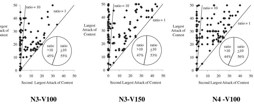
4.3. Guerillas In Our Midst

While it is clear that subjects are not behaving in strict accordance with the theoretical

predictions, is there some consistency to how they behave? For attackers, there is anecdotal

evidence to suggest that many people are behaving like guerillas, focusing their investments on

one intense attack. Figure 2 plots the largest and second largest attacks for every contest lasting

at least three battles for each treatment.24 Nearly half of these contests are such that the largest

attack is at least 10 times greater than the next largest attack.25 _{For comparison, the ratio of the}

largest defense to the second largest defense is less than 2 for more than 90% of these same

contests. Kovenock et al. (2010) also report behavior consistent with guerilla attacks in the

simultaneous weakest-link contest. Chowdhury et al. (2011) report similar behavior in

constant-sum Colonel Blotto games between asymmetric players. Together these results suggest such

behavior is a robust strategy when attacking weakest-link systems.

5. Conclusions

Numerous systems in society can be described as weakest-link networks, where a single

breach can destroy the entire system. For example, in preventing airplane hijackings, passenger

screening inside the terminal at Los Angeles International Airport (LAX) is only valuable if a

(XNA). Recently, attention has been given to modeling the optimal strategies of those who wish

to protect weakest-link systems and those who wish to destroy them. However, that work has

been focused on the case where the attacker is deciding among targets and the defender has to

protect all potential targets concurrently. In this paper we consider the case where battles occur

sequentially, a game of siege. For example, an employer has to retain its skilled employees

every period and it is not enough for the army to prevent the overthrow of the government once.

In our model, a battle is won by the party investing more, but the defender has to win the

entire series of battles to win the contest while the attacker needs to win only once. Within this

structure, the continuation value of the defender is increasing within each battle won as the

number of future battles that must be won is decreasing. If the horizon is too long, the defender

should optimally choose to concede in the first battle. If the horizon is sufficiently short, then

the defender will put up a fight in every battle, but the intensity of the defense should not change

as the end approaches. Thus, the decision of defenders when they first come under assault is one

of “fight or flight.” Somewhat counter intuitively, when facing a fight the intensity of the assault

should decrease over time. These predictions are dramatically different from the existing

literature on simultaneous battle contest where attackers concentrate on a single target and

defenders are forced to randomize their protection of each target.

This study also reports the results of a series of laboratory experiments designed to test

the theoretical predictions of our model. In our baseline treatment, defenders should fight. Our

two alternative treatments have either more battles or a lower payoff to the defender for winning,

both of which should cause defenders to prefer flight. We find that contest outcomes are largely

consistent with the theory. Results 1 and 2, respectively, show that defenders are more likely to

smaller. Result 6 shows that defenders are more likely to win battles as the contest progresses.

However, Results 3, 4, and 5, which deal with individual behavior, are not consistent with the

theoretical predictions. What we observe is that subjects in both roles tend to over invest,

driving profits down (Result 3). Further, defenders are reluctant to flight when they should

(Result 4) and tend to actually increase their effort as the contest progresses (Result 5).

Attackers also increase their investments as the contest progresses (Result 5), contrary to the

theoretical predictions. It also appears that attackers engage in concentrated assaults suggesting

that the guerilla behavior reported by Kovenock et al. (2010) and Chowdhury et al. (2011) is a

robust phenomenon when people are attacking weakest-link systems.

We believe that the connection between behavior and theory is an important area for

future research. A partial explanation of observed behavior for which there is some support from

previous laboratory experiments (Sheremeta, 2010a, 2010b; Price and Sheremeta, 2011) is that

subjects place a positive value on “winning” battles distinct from the prize money even when no

one receives public recognition for victories. Such motivation could explain why defenders are

reluctant to flight, but cannot explain guerilla attacks since a utility for winning simply shifts

payoffs. Another way in which subjects may differ from the bidders in the model is in their risk

attitudes. While the theory assumes risk neutral agents, many laboratory studies have found that

people behave as if they are risk averse (Holt and Laury, 2002; Sheremeta and Zhang, 2010;

Sheremeta, 2011). However, risk aversion should encourage defenders to flight and not to fight.

Similarly, previous experiments have found that people have difficulty backwards inducting in

new situations, but typically learn to do so with modest experience (Camerer, 2003). However,

we do not observe improved performance with experience. Observed behavior may be due to

field and in the laboratory experiments (Croson and Sundali, 2005; Sheremeta and Zhang, 2010).

Another potential explanation may be that bidders act as if they or their opponent have a resource

constraint across all battles in a contest.26 For example, due to psychological reasons bidders

may be unwilling to spend more in total than the value of the contest. These conjectures are

intriguing and they suggest a number of avenues for future theoretical work.

References

Avrahami, J., and Y. Kareev. “Do the Weak Stand a Chance? Distribution of Resources in a

Competitive Environment.” Cognitive Science 33 (2009): 940-50.

Baye, M., D. Kovenock and C. de-Vries. “The All-Pay Auction with Complete Information.”

Economic Theory 8 (1996): 291-305.

Bier, V., S. Oliveros and L. Samuelson. “Choosing What to Protect: Strategic Defensive

Allocation against an Unknown Attacker.” Journal of Public Economic Theory 9 (2007):

563-87.

Budd, C., C. Harris and J. Vickers. “A Model of the Evolution of Duopoly: Does the Asymmetry

Between Firms Tend to Increase or Decrease?” Review of Economic Studies 60 (1993):

543-73.

Camerer, C. Behavioral Game Theory: Experiments in Strategic Interaction. Roundtable Series

in Behavioral Economics. Princeton: Princeton University Press, 2003.

Chowdhury, S., D. Kovenock and R. Sheremeta. “An Experimental Investigation of Colonel

Blotto Games.” Economic Theory, forthcoming (2011).

Clark, D. and K. Konrad. “Asymmetric Conflict: Weakest Link Against Best Shot.” Journal of

Conflict Resolution 51 (2007): 457-69.

Cooper, J., and R. Restrepo. “Some Problems of Attack and Defense.” Siam Review 9 (1967):

680-91.

Coughlin, P. “Pure Strategy Equilibria in a Class of Systems Defense Games.” International

Journal of Game Theory 20 (1992): 195-210.

Croson, R. and J. Sundali. “The Gambler’s Fallacy and the Hot Hand: Empirical Data from

Davis, D., and R. Reilly. “Do Many Cooks Always Spoil the Stew? An Experimental Analysis of

Rent Seeking and the Role of a Strategic Buyer.” Public Choice 95 (1998): 89-115.

Fischbacher, U. “z-Tree: Zurich Toolbox for Ready-Made Economic Experiments.”

Experimental Economics 10 (2007): 171-8.

Friedman, D., K. Pommerenke, R. Lukose, G. Milam, B. Huberman. “Searching for the Sunk

Cost Fallacy.” Experimental Economics 10 (2007): 79-104.

Fudenberg, D., R. Gilbert, J. Stiglitz and J. Tirole. “Preemption, Leapfrogging and Competition

in Patent Races.” European Economic Review 22 (1983): 3-31.

Glazebrook, K., and A. Washburn. “Shoot-Look-Shoot: A Review and Extension.” Operations

Research 52 (2004): 454-63.

Gneezy, U., and R. “All-Pay Auctions – An Experimental Study.” Journal of Economic Behavior

and Organization 61 (2006): 255-75.

Gross, O. Targets of Differing Vulnerability with Attack Stronger than Defense. RM-359,

RAND Corporation, Santa Monica. 1950.

Harris, C. and J. Vickers. “Perfect Equilibrium in a Model of a Race.” Review of Economic

Studies 52 (1985): 193-209.

Harris, C. and J. Vickers. “Racing with Uncertainty.” Review of Economic Studies 54 (1987):

1-21.

Hart, S. “Discrete Colonel Blotto and General Lotto Games.” International Journal of Game

Theory 36 (2008): 441-60.

Herrmann, B. and H. Orzen. “The Appearance of Homo Rivalis: Social Preferences and the

Hillman, A. and J. Riley. “Politically Contestable Rents and Transfers.” Economics and Politics

1 (1989): 17-40.

Hirshleifer, J. “From Weakest-Link to Best-Shot: the Voluntary Provision of Public Goods.”

Public Choice 41 (1983): 371-86.

Holt, C. and S. Laury. ”Risk Aversion and Incentive Effects.” American Economic Review 92

(2002): 1644-55.

Konrad, K. and D. Kovenock. ”Multi-Battle Contests.” Games Economic Behavior 66 (2009):

256-74.

Kovenock, D. and B. Roberson. “Terrorism and the Optimal Defense of Networks of Targets.”

Miami University, mimeo. (2010).

Kovenock, D., B. Roberson and R. Sheremeta. “The Attack and Defense of Weakest-Link

Networks.” Chapman University, Working Paper. (2010).

Kremer, M. “The O-Ring Theory of Economic Development.” Quarterly Journal of Economics,

108 (1993): 551- 75.

Kvasov, D. “Contests with Limited Resources.” Journal of Economic Theory 127 (2007):

738-48.

Lei, V., C. Noussair, and C. Plott. “Nonspeculative Bubbles in Experimental Asset Markets:

Lack of Common Knowledge of Rationality vs Actual Irrationality.” Econometrica 69

(2001): 831-59.

Leininger, W. “Patent Competition, Rent Dissipation, and the Persistence of Monopoly: the Role

of Research Budgets.” Journal of Economic Theory 53 (1991): 146-72.

Levitin, G. and K. Hausken. “Resource Distribution in Multiple Attacks Against a Single

Lugovskyy, V., D. Puzzello, and S. Tucker. “Experimental Investigation of Overdissipation in

the All Pay Auction.” European Economic Review 54 (2010): 974-997.

Moore, T., R. Clayton and R. Anderson. “The Economics of Online Crime.” Journal of

Economic Perspectives 23 (2009): 3–20.

Potters, J., C. De Vries and F. Van Linden. “An Experimental Examination of Rational Rent

Seeking.” European Journal of Political Economy 14 (1998): 783-800.

Price, C. and R. Sheremeta. “Endowment Effects in Contests.” Economics Letters 111 (2011):

217–219.

Roberson, B. “The Colonel Blotto Game.” Economic Theory 29 (2006): 1-24.

Sheremeta, R. “Contest Design: An Experimental Investigation,” Economic Inquiry 49 (2011):

573–90.

Sheremeta, R. “Expenditures and Information Disclosure in Two-Stage Political Contests.”

Journal of Conflict Resolution 54 (2010a): 771-798

Sheremeta, R. “Experimental Comparison of Multi-Stage and One-Stage Contests.” Games and

Economic Behavior 68 (2010b): 731-747.

Sheremeta, R. and J. Zhang. “Can Groups Solve the Problem of Over-Bidding in Contests?”

Social Choice and Welfare 35 (2010) 175-197.

Shubik, M. and R. Weber. “Systems Defense Games: Colonel Blotto, Command and Control.”

Naval Research Logistics Quarterly 28 (1981): 281-287.

Snyder, J. “Election Goals and the Allocation of Campaign Resources.” Econometrica 57 (1989):

637-60.

Szentes, B. and R. Rosenthal. “Three-Object Two-Bidder Simultaneous Auctions: Chopsticks

Appendix: Tables and Figures

Table 1: Equilibrium Payoffs and Expenditures

Battle Expected Payoff Expected Expenditure Probability of Winning

Player 𝐷 Player 𝐴 Player 𝐷 Player 𝐴 Player 𝐷

Panel A: Battle n − k for 𝑣_𝐷 ≥ 𝑛𝑣_𝐴

𝑛 − 𝑘 𝑣𝐷− (𝑘 + 1)𝑣𝐴 0 𝑣₂𝐴 (𝑣𝐴)

2

2(𝑣𝐷− 𝑘𝑣𝐴) 1 −

𝑣𝐴

2(𝑣𝐷− 𝑘𝑣𝐴)

Panel B: Battle 1 for 𝑛𝑣_𝐴> 𝑣_𝐷> (𝑛 − 1)𝑣_𝐴

1 0 𝑛𝑣_𝐴− 𝑣_𝐷 (𝑣𝐷− (𝑛 − 1)𝑣𝐴)

2

2𝑣𝐴

𝑣𝐷− (𝑛 − 1)𝑣𝐴

2

𝑣𝐴

2(𝑣𝐷− (𝑛 − 1)𝑣𝐴)

Panel C: Battle 1 for (𝑛 − 1)𝑣_𝐴≥ 𝑣_𝐷

Table 2: Equilibrium Predictions and Aggregate Statistics

Treatment

(𝑛, 𝑣_𝐷, 𝑣_𝐴)

Battle Number

Average Allocation Payoff Probability of

Winning a Battle

Probability of Winning the Game Equili-

brium Actual

Equili-

brium Actual

Equili-

brium Actual

Equili-

brium Actual

D A D A D A D A D D D D

N3-V100 (3, 100, 50)

1 0.0 0.1 15.0 12.4

0 50 -7.5 11.6

0.00 0.55

0.00 0.29

2 25.0 25.0 20.1 11.1 0.50 0.70

3 25.0 12.5 26.7 14.6 0.75 0.75

N3-V150 (3, 150, 50)

1 25.0 25.0 26.8 18.0

0 0 -6.7 -6.0

0.50 0.65

0.31 0.41

2 25.0 12.5 32.6 13.0 0.75 0.79

3 25.0 8.3 39.2 17.0 0.83 0.80

N4-V150 (4, 150, 50)

1 0.0 0.1 18.4 13.1

0 50 -17.4 3.2

0.00 0.63

0.00 0.27

2 25.0 25.0 22.5 12.0 0.50 0.74

3 25.0 12.5 28.6 15.2 0.75 0.73

Figure 1: Total Expenditure across All Periods (All Treatments)

0

10

20

30

40

50

60

70

1

3

5

7

9

11

13

15

17

19

Ex

pendi

tur

e

Figure 2: Attacks Lasting for at least Two Battles by Treatment

N3-V100 N3-V150 N4 -V100

0 10 20 30 40 50

0 10 20 30 40 50 Largest

Attack of Contest

Second Largest Attack of Contest ratio = 10

ratio = 1

ratio >10 45% ratio <10 55% 0 10 20 30 40 50

0 10 20 30 40 50 Largest

Attack of Contest

Second Largest Attack of Contest ratio = 10

ratio = 1

ratio >10 47% ratio <10 53% 0 10 20 30 40 50

0 10 20 30 40 50 Largest

Attack of Contest

Second Largest Attack of Contest ratio = 10

ratio = 1

Figure A1: Expenditures in Each Battle across All Periods (N3-V100 Treatment)

Defender Expenditures

Attacker Expenditures

0

10

20

30

40

1

3

5

7

9

11

13

15

17

19

Ex

pendi

tur

e

Period

Battle 1 (D)

Battle 2 (D)

Battle 3 (D)

0

10

20

30

40

1

3

5

7

9

11

13

15

17

19

Ex

pendi

tur

e

Figure A2: Expenditures in Each Battle across All Periods (N3-V150 Treatment)

Defender Expenditures

Attacker Expenditures

0

10

20

30

40

50

1

3

5

7

9

11

13

15

17

19

Ex

pendi

tur

e

Period

Battle 1 (D)

Battle 2 (D)

Battle 3 (D)

0

10

20

30

40

50

1

3

5

7

9

11

13

15

17

19

Ex

pendi

tur

e

Figure A3: Expenditures in Each Battle across All Periods (N4-V150 Treatment)

Defender Expenditures

Attacker Expenditures

0

10

20

30

40

50

1

3

5

7

9

11

13

15

17

19

Ex

pendi

tur

e

Period

Battle 1 (D)

Battle 2 (D)

Battle 3 (D)

Battle 4 (D)

0

10

20

30

40

50

1

3

5

7

9

11

13

15

17

19

Ex

pendi

tur

e

Battle 1 (A)

Battle 2 (A)

Online Appendix B: Instructions for N3-V100

General Instructions

This is an experiment in the economics of decision making. Various research agencies have provided the funds for this research. The instructions are simple and if you follow them closely and make careful decisions, you can make an appreciable amount of money.

The currency used in the experiments is called Francs. At the end of the experiment your Francs will be converted

to US Dollars at the rate 25 Franks = US $1. You are being given a $20 participation payment. Any gains you

make will be added to this amount, while any losses will be deducted from it. You will be paid privately in cash at the end of the experiment.

It is very important that you do not communicate with others or look at their computer screens. If you have questions, or need assistance of any kind, please raise your hand and an experimenter will approach you. If you talk or make other noises during the experiment you will be asked to leave and you will not be paid.

Instructions for the Experiment

The experiment consists of 20 decision tasks. At the beginning of the first task you will be randomly assigned the

role of participant 1 or participant 2. You will remain in this role for the first 10 decision tasks and then change

your role assignment for the last 10 tasks of the experiment. For each task you will be randomly paired with another

participant in the experiment who is in the opposite role. There are 16 participants in the experiment so 8 are in

each role. For each task you are equally likely to be paired with any of the 8 participants in the other role, but no participant will be able to identify if or when he or she has been paired with a specific person.

The Decision Task

For each decision task there is a reward in Francs for participant 1 and a reward in Francs for participant 2. These rewards are not the same for the two participants. Only one of the participants will receive the reward for a given

task. The reward to participant 1 is 100 Francs and the reward to participant 2 is 50 Francs.

Each task involves up to 3 rounds. In each round, both participants allocate Francs, and whoever allocates more

Francs wins that round with ties being broken randomly. A participant’s allocation cannot exceed his or her reward

so allocations can be anything from [0, 0.1, 0.2, …, the reward]. So for example, if participant 1 allocates 11.4

Francs and participant 2 allocates 11.3 francs, then participant 1 will win the round.

Your Earnings

If participant 1 wins all 3 rounds then he or she receives the reward. However, if participant 2 wins any round, then

participant 2 receives the reward. Since participant 2 only needs to win a single round, the task will end if this occurs. Notice that a single reward is received for the whole task; there is not a reward for each round.

Any Francs allocated in a round are deducted from your payment regardless of whether or not you won the round or the reward. This means that if both participants allocate Francs in a task, then one will lose Francs. This is why

each participant is being given a participation payment of $20, which corresponds to 500 Francs.

Consider the following example where the reward to participant 1 is 100 and the reward to participant 2 is 50 and the task involves 3 potential rounds. If participant 1 allocates 15 Francs in round 1 and participant 2 allocates 5 Francs in round 1 then participant 1 wins the round and both participants lose their allocations. If in the second round participant 1 allocates 10 Francs and participant 2 allocates 15 Francs then participant 2 wins the round and

hence receives the reward. Participant 1’s earnings for the task would be –15 – 10 = –25 Francs and Participant 2’s

earnings for the task would be 50 – 5 – 15 = 30 Francs.

Notes

1 _{For a review of the literature see Roberson (2006). Some examples of simultaneous games of}

attack and defense are Gross (1950), Cooper and Restrepo (1967), Shubik and Weber (1981),

Snyder (1989), Coughlin (1992), Szentes and Rosenthal (2003), Bier et al. (2007), Kvasov

(2007), and Hart (2008).

2 _{The main distinction between the two papers is that Clark and Konrad (2007) assume the}

probability of winning a given battle is proportional to investment, while Kovenock and

Roberson (2010) assume that victory is deterministic.

3 _{The subsequent papers of Harris and Vickers (1985, 1987), Leininger (1991), Budd et al.}

(1993), and Konrad and Kovenock (2009) investigate different factors that affect behavior in the

sequential multi-battle contests.

4 _{Similar problems h}ave been studied in the “shoot_-look-shoot problem” literature (for a review

see Glazebrook and Washburn, 2004). However, those models assume that the probability of

winning a battle does not depend on the defender’s and the attacker’s efforts.

5 _{This is mainly because the defender’s valuation of the overall contest in early battles is}

relatively low, since the defender has to be successful in each battle and there are still many

battles to go. However, as the defender wins early battles, his valuation for continuing the contest

increases and thus the attacker becomes discouraged. As a result, the probability of winning

future battles by the attacker decreases, while the probability of winning future battles by the

defender increases.

6 _{It is interesting to compare our results to the simultaneous battle game of attack and defense by}

Kovenock and Roberson (2010). In particular, when 𝑣_𝐷 ≥ 𝑛𝑣_𝐴, the expected payoffs of the

Nevertheless, the strategic behavior in two games is quite different. In particular, Kovenock and

Roberson (2010) find that the attacker utilizes a stochastic guerilla warfare strategy in which,

with probability one, the attacker engages in only one single battle. On the contrary, in our

model, the attacker always has an incentive to fight in each battle.

7Konrad and Kovenock (2009) call such a break point a ‘separating state.’ Their theoretical

model of a contest with intermediate prizes is more general than the model studied in the current

paper. In fact, some of the results provided in our paper can be derived from Konrad and

Kovenock (2009).

8 _{Note that this is never the case in the simultaneous game of attack and defense by Kovenock}

and Roberson (2010). In particular, under all parameters, the optimal strategy for the defender is

to stochastically fight with positive probability in all battles, allocating random, but positive,

resource levels in each battle. On the contrary, in our model, when (𝑛 − 1)𝑣_𝐴 ≥ 𝑣_𝐷, the defender

gives up with probability one, by allocating zero resources in the first battle.

9 _{To demonstrate that (0, 𝜀) is a Nash equilibrium strategy profile for players 𝐷 and 𝐴, see that}

the expected payoff in battle 2 for player 𝐷 is 0 and the expected payoff for player 𝐴 is positive,

i.e. 𝑣 = (𝑛 − 1)𝑣_𝐴− 𝑣_𝐷 > 0. Therefore, in battle 1, players 𝐷 and 𝐴 compete in a simultaneous

move all-pay auction, where player 𝐷’s value is 0 and player 𝐴’s value is 𝑣. It is a strictly

dominant strategy for player 𝐷 to make an expenditure of 0, which assures that played 𝐷

receives a payoff of 0. Making any expenditure 𝜀 > 0 guarantees a sure loss of 𝜀, because losing

the battle yields no benefit and costs 𝜀 and winning the battle has an expected value of 0 and the

cost is still 𝜀. On the other hand, player 𝐴’s dominant strategy is to assure the victory of the prize

dominant strategy for player 𝐴 if the rule was to allocate a victory to player 𝐴 with certainty in

case of a tie (Roberson, 2006; Konrad and Kovenock, 2009). However, given that ties are broken

randomly, player 𝐴’s dominant strategy is to make the lowest possible expenditure of 𝜀 > 0 (0.1

francs in our experiment) to guarantee the payoff of 𝑣 at the minimal cost of 𝜀. This choice is

better than making an expenditure of 0 and receiving an expected payoff of 𝑣/2, i.e. 𝑣 − 𝜀 >

𝑣/2. Therefore, neither of the players has an incentive to deviate from the equilibrium profile

(0, 𝜀).

10 _{This suggests that attackers want to stretch out the duration of the contest. Indeed, this tactic}

has often been applied in historic games of siege. However, various constraints such as a food

supply or weather often prevent he attacker from forcing the contest to continue indefinitely.

11 _{For the defender, the value of being at period 𝑡is 𝑣}

𝐷𝑡 = 𝑚𝑎𝑥{0, 𝑝𝑣𝐷𝑡+1+ (1 − 𝑝)0 − 𝑑}, where

𝑝denotes the chance of the defender winning the battle given both players’ investments and 𝑑

denotes the expected investment by the defender. Since 𝑣_𝐷𝑡 = 𝑣_𝐷𝑡+1 this equation implies that

𝑣𝐷𝑡 = 𝑣𝐷𝑡+1= 0 and the defender should surrender so that 𝑝 = 0. For the attacker, the value of

being at period 𝑡 is 𝑣_𝐴𝑡 = 𝑚𝑎𝑥{0, 𝑝𝑣_𝐴𝑡+1+ (1 − 𝑝)𝑣_𝐴− 𝑎}, where 𝑎 is the attacker’s expected

investment. The attacker will choose to attack if 𝑣_𝐴𝑡 is positive, which is the same condition as

𝑣𝐴 being positive since 𝑝 = 0 and 𝑎 ≥ 0 can be arbitrarily small.

12 _{The experimental instructions used context neutral language. The instructions are available in}

an online appendix.

13 _{Placing a theoretically nonbinding upper limit on bids may have some psychological impact on}

potential loss of control due to bankruptcy (as described at the end of this section) were

considered to be more important.

14 _{By randomly selecting periods for payment, the size of the endowment is smaller than it would}

be if subjects were paid for each contest. Given the restriction that bids could not exceed value

in any round and the other features of the experimental design it was not possible for subjects to

go bankrupt.

15 _{We used two different variables for a period trend, one for the first 10 periods and one for the}

last 10 periods of the experiment. The two variables were used since subjects changed their role

assignments after the first 10 periods of the experiment.

16 _{A standard Wald test, conducted on estimates of panel regression models, rejects the}

hypothesis that the average payoffs in N3-V100, N3-V150, and N4-V150 treatments are equal to

the predicted theoretical values in Table 4 (p-values < 0.05). The panel regression models

included a random effects error structure, with a random effect for each individual subject, to

account for the repeated measures nature of the data. The standard errors were clustered at the

session level to account for session effects. The two separate period trends were used to control

for learning for the first 10 periods and the last 10 periods of the experiment.

17 _{In our experiment, subjects who get to the last battle have already made some expenditures in}

the previous battles. If the sunk cost hypothesis is true, it will entail that subjects who expend

more in previous battles are also more likely to expend more in the last battle – to recoup some

of their expenditure. A simple random effect model finds that for the defender there is a positive

relationship between expenditure in battle 3 and total expenditure in the previous battles 1 and 2

Therefore, we conclude that the sunk cost fallacy is not likely to be the main consistent force

driving the over-expenditures in our experiment.

18 _{Of course, it may be that changes to behavior due to learning require more experience than}

provided in our experiment.

19 _{A reluctance to bid 0 could be due to the active participation hypothesis (see Lei et al., 2001),}

which argues that subjects who come to laboratory experiments want to do something.

20 _{We estimate a panel regression model separately for each treatment and player type. Each}

model included random effects for each individual subject and standard errors were clustered at

the session level. The two separate period trends were used to control for learning for the first 10

periods and the last 10 periods of the experiment. The independent variable is bid and the main

dependent variable is the battle number. For the defender, the battle number variable is positive

and significant in all treatments (p-values < 0.05). For the attacker, the battle number variable is

positive and significant in treatments N3-V100 and N4-V150 (p-values < 0.05), but not in

treatment N3-V150.

21 _{Theoretically, this discouragement effect is the driving force behind the predictions of our}

model (Baye et al., 1996). The idea behind the discouragement effect is straightforward: the

player with the higher valuation imposes a strong discouragement effect on the player with the

lower valuation. As the result, the player with the lower valuation reduces his expenditures.

22The defender’s valuation _{for continuing the contest increases in the number of battles won and}

thus the attacker becomes discouraged.

23 _{We estimate a probit panel regression model separately for each treatment, using subject}

defender won the battle and the main dependent variable is the battle number. The battle number

variable is positive and significant in all treatments (p-values < 0.05). Obviously, the probability

of the attacker winning each battle is simply one minus the probability of winning that battle by

the defender. So, the same statistical conclusions carry on to the attackers.

24 _{Any contest that ends after the first battle is trivially consistent with a guerilla attack. Also,}

any attacker following the equilibrium strategy in N3-V100 or N4-V150 and winning the second

battle would appear to be a guerrilla based upon the metric used in Figure 2. Therefore the three

panels in Figure 2 only include contests that lasted at least 3 battles, although they are

qualitatively unchanged if contests lasting for only two battles are included.

25 _{For defenders, individual behavior is similar to the aggregate pattern discussed above where}

defense tends to increase with each successive battle.