What Caused the Decline in the US Saving Ratio?

Munich Personal RePEc Archive

What Caused the Decline in the US

Saving Ratio?

Paradiso, Antonio and Rao, B. Bhaskara

5 January 2011

1998 words

What Caused the Decline in the US Saving Ratio?

Antonio Paradiso

[email protected]

Department of Economics

University of Rome La Sapienza, Rome (Italy)

B. Bhaskara Rao

[email protected]

School of Economics and Finance

University of Western Sydney, Sydney (Australia)

Abstract

We investigate whether the mortgage equity withdrawal (MEW) mechanism is useful

for explaining the large declines in the US personal saving ratio in the last two decades.

MEW depends on house price inflation and mortgage rates. In addition stock prices

may affect saving ratio. Therefore, we estimate a VEC model with these four variables.

The impulse response analysis shows that saving ratio decreases with positive shocks to

asset prices and increases with positive shocks to mortgage rates.

Keywords: Saving ratio, MEW, VEC, asset prices, interest rates

1. Introduction

The average US personal saving rate during 1960-1985 was about 9% but it has declined to 2.5% by

2007. Different explanations are offered for this large reduction; see Guidolin and La Jeunesse

(2007). A theory advanced by some practitioners is the mortgage equity withdrawal (MEW)

hypothesis of Hatzius (2006). MEW argues that equity extracted from existing houses, via cash-out

refinancing, is the main cause for the declining saving pattern. MEW acts as an additional channel,

beyond the wealth effect, through which increases in house prices can boost consumer spending.

We show that theratio of MEW toincome depends positively on the change in house prices and

negatively on mortgage rate.

To examine the role of MEW in the personal saving rate, a VEC model is estimated with the

saving rate, the two variables explaining MEW and the stock price index and the results confirm the

presence of a significant long-run relationship. Next, we identify the effects of shocks on the saving

rate by imposing plausible long-run restrictions on the estimated VEC. The impulse response

functions (IRFs) show that saving rate reacts negatively to asset price shocks and positively to

mortgage rate shocks.

2. The empirical VEC model

The variable of the empirical VEC analysis are: the house price index inflation (expressed in the

year-on-year growth rate) ₄ h,

p the Standard and Poor’s 500 index (expressed in log)sp500,the

mortgage rate imtg,and the personal saving ratiosav. For the house price index the source was

Standard and Poor’s/Case–Shiller, whereas for others the FRED (Federal Reserve Economic Data). We use observations from 1988Q1 to 2010Q1.

The choice of house price inflation and mortgage rate is not ad hoc. MEW depends mainly

on these two variables. Home equity can be extracted if either of the two following events occur: 1)

the value of the house increases; 2) the current mortgage rate goes below the historically contracted

one. In such cases the mortgage can be renegotiated, increasing the loan amount or decreasing the

service of debt, and then freeing resources.1 Our view of the MEW mechanism is confirmed by

1

DOLS (dynamic OLS) estimation in Table 1. MEW, expressed as a share of disposable income, can

be explained with ₄ h and mtg.

p i

(Table 1 here)

2.1 Reduced-form model

First, ADF unit roots tests are conducted for the variables before proceeding with the reduced form

model specifications. AIC criteria is used in determining the lag orders. The results (available upon

request) show that at the 5% level,the unit root null for the variables in levels is not rejected, while

the null is rejected for their first differences. Therefore, cointegration between these variables

( , 500, ₄ h

sav sp p and mtg

i _{) is possible. The next step is the specification of an unrestricted VAR}

model for the cointegration tests:

0 1

1

p

t t t

i

y v y u (1)

where yt imtg, 4ph,sp500,sav '. All the information criteria (AIC, SIC, HQ) suggest that 2,

and a series of diagnostic tests are in Table 2.

(Table 2 here)

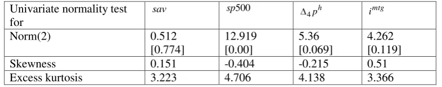
We test against autocorrelation, non-normality, and ARCH effects in the VAR(2) residuals.

The results are satisfactory, except for some traces of non-normality. To examine whether lack of

normality is associated with specific variables, univariate tests are used in Table 3. Normality is

rejected because of non-normality in the stock prices and this is due to an excess of kurtosis. An

absolute value of unity or less for skewness is acceptable according to Juselius (2006). Since

Johansen’s maximum likelihood (ML) approach appears robust to excess kurtosis, non-normality is not a serious problem; see Juselius (2001).

(Table 3 here)

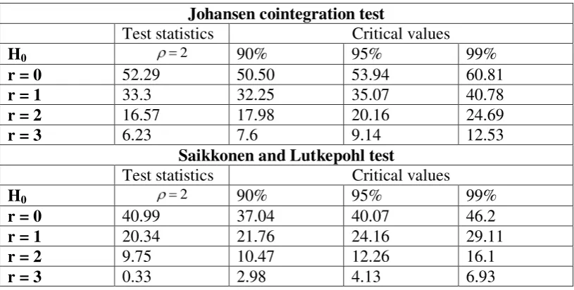
We test for cointegration of the VAR(2) specification with the Johansen (1995) trace and

the Saikkonen and Lutkepohl (2000) tests, with only a constant as the deterministic term. Results in

Table 4 show that both the multivariate cointegrating tests reject zero cointegrating relations, while

the existence of one cointegrating vector is not rejected.

(Table 4 here)

The VECM based on the VAR(2), under the rank restriction r = 1, can be specified as:

1 '

1 0 1

p

t t i t i t

i

y y y u (2)

Table 5 shows the Johansen ML estimate of the cointegrating relation, where the exclusion

of the insignificant parameters is based on the top-down algorithm ( AIC criteria) and it is

normalized on the saving ratio. This cointegrating vector is the long run equilibrium relationship

between the saving rate stock price, house price inflation, and the nominal interest rate. All the

coefficients are statistically significant and have the expected signs. Also, the estimates of the

adjustment coefficients ( )has the correct negative sign and significant at the 1% level.2 This is an

important evidence that the variables explaining MEW viz., house price inflation and mortgage

rate, play an important role in explaining the saving ratio in our sample.

(Table 5)

2.2 Structural identification and impulse response analysis

2

Having specified the reduced-form model, we now examine the structural analysis. In the VEC

framework the following restrictions are needed to analyze the effects of structural shocks with the

moving average representation of the model:3

*

1

( )

t

t t t

i

L

x (3)

where the matrix CB represents the permanent component of the model, and the matrix

polynomial *_{( )L C}*_{( )L Bthe transitory or cyclical component. The vector of the structural shocks}

is given by

' 500

, h, ,

i p sp sav

t . We proceed to identify the shocks by imposing restrictions on

the long-run impact matrix CB:

* 0 0 0 * * 0 0 * * * 0 * * * 0

CB

We need 1 ( 1) 6

2K K linearly independent restrictions. Cointegration analysis suggests that

the saving ratio is stationary. Accordingly, saving shocks have no long-run impact on the other

variables, which correspond to four zeros in the last column of the matrix CB. This reduces the

rank of CB, and implies K* 3 linearly independent restrictions. To identify the K* 3 permanent

shocks, K*(K* 1)/ 2 3 additional restrictions are necessary. We assume that the long-term interest

rate influences asset prices in the long run, but not the opposite. This is because long-term interest

rates commove mainly with fed funds in the long period (Mehra, 1996) and the Fed does not target

asset prices directly (Bernanke and Gertler 1999). The last assumption is that house prices are more

exogenous than stock prices, that is, stock prices respond to house price shocks, but the opposite is

not true. This assumption comes from the fact that in the last 20 years the housing market seems to

have had a more independent dynamics (Leamer 2008).4

3

For a derivation see Lutkepohl and Kratzick (2004).

4

However, we have proved that the position can be changed between sp500 and 4ph and the results do not change.

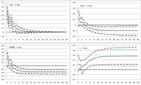
Figure 1 shows the responses of the saving ratio to a stock price, house price inflation, and

mortgage rate shock together with 95% bootstrap confidence intervals based on 2000 replications

over a simulation period of 30 quarters. The signs of the dynamic responses are as expected. A

positive saving ratio shock has a significant positive impact on itself for about two years. In the long

run there is no significant effect, which is in line with the restriction in the long-run matrix. A

positive stock price shock, instead, causes an initial positive response of the saving rate, but it is

insignificant. The effect on the saving ratio becomes negative and significant only after about four

quarters. In the long run this effect remains significant. Similar observations apply to a positive

shock to house price inflation. Finally, the saving ratio increases after a shock to the mortgage rate

and is significant after about 4 quarters.

(Figure 1 here)

Overall, IRF analysis suggests that: (a) asset prices and mortgage rate shocks have an impact

on saving with some delay; (b) MEW shocks have played an important role in saving during the last

20 years.

3. Conclusions

In this paper we have investigated the dynamics of the personal saving ratio in the US economy for

the last two decades, a period of huge declines in the saving ratio. We found that the variables

explaining the MEW, viz., house price inflation and mortgage rate, and stock prices enter the

long-run relationship of the saving ratio. We have estimated with VEC this long long-run relationship and a

structural form with restrictions on the long-run impact matrix. Impulse responses showed that the

saving ratio responds negatively to asset price shocks and positively to mortgage rate shocks and

these are consistent with the underlying theories and empirical results.

References

Bernanke, B. S., and Gertler, M. 1999. Monetary policy and asset price volatility. Federal Reserve Bank of Kansas City Economic Review 4: 17–53.

Greenspan, A., and Kennedy, J. 2008. Sources and uses of equity extracted from homes. Oxford Review of Economic Policy 24: 120–144.

Guidolin, M., and La Jeunesse 2007. The decline of the U.S. personal saving rate: Is it real and is it a puzzle? Federal Reserve Bank of St. LouisReview 89: 491–514.

Hatzius, J. 2006. Housing holds the key to Fed policy. Global Economics Paper No. 37, Goldman Sachs.

Johansen, S. 1995. Likelihood-based inference in cointegrated vector autoregressive models. Oxford: Oxford University Press.

Juselius, K. 2001. Big shocks, outliers and interventions. A cointegration and common trends analysis of daily bond rates. Mimeo, European University Institute, Florence.

Juselius, K. 2006. The cointegrated VAR model: Methodology and applications. Oxford: Oxford University Press.

Leamer, E. E. 2008. Housing is the business cycle. Proceedings, Federal Reserve Bank of Kansas City: 359–413.

Mehra, Y. P. 1996. Monetary policy and long-term interest rates. Federal Reserve Bank of Richmond Economic Quarterly 82: 27–49.

Lutkepohl, L., and Kratzick, M. 2004. Applied time series econometrics. Cambridge: Cambridge University Press.

Appendix: Tables and figures

Table 1: DOLS estimates of active MEW

Model _t / _{t t 0 1t}mtg _{2 4 t}h k _{1,j t j}mtg k _2,j ( _{4 t j}h ) _t

j k j k

amew yd MEWRAT i p i p

Long-run relation MEWRAT_{t 0 1}i_tmtg _{2 4}p_th u_t

Sample Period 0 1 2

1991q1–2008q2 -3.744* -0.298*** 0.099***

Phillips–Ouliaris test -4.23***

Note: *, **, *** represent, respectively, the significance levels of 10%, 5%, and 1%. amew and yd

are expressed in natural logarithm. Leads and lags of DOLS estimations are selected according to HQ criteria. The sample period denotes the range of data before the data points for leads and lags are removed. Newey–West corrected t-statistics are applied in regression.

Table 2: Diagnostic tests for VAR(2) specifications

16

Q *

16

Q LM5 LJB₄L MARCHLM(5)

2 _210.7

[0.73] 234.38 [0.30] 95.96 [0.11] 19.82 [0.01] 549.0 [0.06]

Note: p-values in brackets. Q_p = multivariate Ljiung–Box portmentau test tested up to the th _lag;

LM = LM (Breusch–Godfrey) test for autocorrelation up to the th _lag; L p

LJB = multivariate Lomnicki–Jarque–Bera test for non-normality from Lutkepohl (2004) with pvariables in the

system; MARCH_LM( ) = multivariate LM test for ARCH up to the th lag.

Table 3: Specification tests for VAR(2) model

Univariate normality test for

sav sp500

4ph imtg

Norm(2) 0.512

[0.774] 12.919 [0.00] 5.36 [0.069] 4.262 [0.119]

Skewness 0.151 -0.404 -0.215 0.51

Table 4: Multivariate cointegration tests

Johansen cointegration test

Test statistics Critical values

H0 2 90% 95% 99%

r = 0 52.29 50.50 53.94 60.81

r = 1 33.3 32.25 35.07 40.78

r = 2 16.57 17.98 20.16 24.69

r = 3 6.23 7.6 9.14 12.53

Saikkonen and Lutkepohl test

Test statistics Critical values

H0 2 90% 95% 99%

r = 0 40.99 37.04 40.07 46.2

r = 1 20.34 21.76 24.16 29.11

r = 2 9.75 10.47 12.26 16.1

r = 3 0.33 2.98 4.13 6.93 Notes: Deterministic term: constant in the cointegrating relationship.

Table 5: Cointegration vector and loading parameters for VECM with two lagged differences and cointegrating rank r =1

500 sp

4ph imtg sav constant

-1.6 (3.6)

-0.042 (2.1)

0.469 (2.9)

1 11.48

(2.87) -0.014

(1.78)

-0.276 (1.86)

- -0.404

(5.25)

Figure 1: Impulse response analysis

-0.1 0 0.1 0.2 0.3 0.4 0.5 0.6 0.7

0 2 4 6 8 10 12 14 16 18 20 22 24 26 28 30

savt--> savt

-0.4 -0.2 0 0.2 0.4 0.6 0.8

0 2 4 6 8 10 12 14 16 18 20 22 24 26 28 30 Δ4 pht--> savt

-0.4 -0.3 -0.2 -0.1 0 0.1 0.2 0.3 0.4 0.5 0.6

0 2 4 6 8 10 12 14 16 18 20 22 24 26 28 30

sp500t--> savt

-0.2 -0.1 0 0.1 0.2 0.3 0.4 0.5

0 2 4 6 8 10 12 14 16 18 20 22 24 26 28 30