BIROn - Birkbeck Institutional Research Online
Corbetta, J. and Peri, Ilaria (2018) Backtesting lambda value at risk. The
European Journal of Finance 24 (13), pp. 1075-1087. ISSN 1351-847X.
Downloaded from:
Usage Guidelines:
Please refer to usage guidelines at or alternatively
Backtesting Lambda Value at Risk
Jacopo Corbetta
CERMICS, ´Ecole des Ponts , UPE, Champs sur Marne, France.
Zeliade Systems, 56 rue Jean-Jacques Rousseau, Paris, France.
and
Ilaria Peri
Department of Economics, Mathematics and Statistics, Birkbeck University of London, England
June 17, 2017
Abstract
A new risk measure, Lambda value at risk (ΛV aR), has been recently proposed
as a generalization of Value at risk (V aR). ΛV aRappears attractive for its potential
ability to solve several problems ofV aR. This paper provides the first study on the
backtesting of ΛV aR. We propose three nonparametric tests which exploit different
features. Two tests are based on simple results of probability theory. One test is
unilateral and is more suitable for small samples of observations. A second test is
bilateral and provides an asymptotic result. A third test is based on simulations
and allows for a more accurate comparison among ΛV aRscomputed with different
assumptions on the asset return distribution. Finally, we perform a backtesting
exercise that confirms a higher performance of ΛV aR in respect toV aR especially
when it is estimated with distributions that better capture tail behaviour.
Keywords: backtesting, hypothesis testing, model validation, risk management.
1
Introduction
Risk measurement and its backtesting are matter of primary concern to financial industry.
Value at risk (V aR) has become the most widely used risk measure. Despite its popularity,
after the recent financial crisis, V aR has been extensively criticized by academics and
risk managers. Among these critics, we recall the inability to capture the tail risk and the
lack of reactivity to market fluctuations. Thus, the suggestion of the Basel Committee, in
the consultative document Fundamental review of the trading book (2013), is to consider
alternative risk measures that are able to overcome the V aR’s weaknesses.
A new risk measure, Lambda Value at Risk (ΛV aR), has been introduced by a
the-oretical point of view by Frittelli, Maggis, and Peri (2014). ΛV aR is a generalization
of the V aR at confidence level λ. Specifically, ΛV aR considers a function Λ instead
of a constant confidence level λ, where Λ is a function of the losses. Formally, given a
monotone and right continuous function Λ :R→(0,1), the ΛV aRof the asset return X
is a map that associates to its cumulative distribution function F(x) = P(X ≤ x) the
number:
ΛV aR=−inf{x∈R|F(x)>Λ(x)} . (1)
This new risk measure appears to be attractive for its potential ability to solve several
problems of V aR. First of all, it seems to be flexible enough to discriminate the risk
among return distributions with different tail behavior, by assigning more risk to
heavy-tailed return distributions and less in the opposite case. In addition, ΛV aR may allow
for a rapid changing of the interval of confidence when the market conditions change.
ΛV aR and a first attempt of backtesting based on the hypothesis testing framework
by Kupiec (1995). In this study, the accuracy of the ΛV aR model is evaluated by
considering the maximum of the Λ function as confidence level. However, the level of
coverage provided by the ΛV aR model may not be constant at any time; hence, this
method misses to assess the actual ΛV aRperformance.
The objective of this paper is to propose the first theoretical framework for the
back-testing of ΛV aR. We present three backtesting methodologies which exploit different
features and may be used with different aims. Our tests evaluate if ΛV aR provides an
accurate level of coverage, this means that the probability of a violation occurringex-post
actually coincides with the one predicted by the model. In respect to the hypothesis
test proposed in Hitaj, Mateus, and Peri (2015), we consider a null hypothesis which
better evaluates the benefits introduced by the ΛV aR flexibility. Our tests can be easily
extended to V aR allowing for a proper comparison among the two risk measures.
Two of these tests are based on simple test statistics whose distribution is obtained
by applying results of probability theory. The first test is unilateral and provides more
precise results for shorter backtesting time windows (e.g. 250 observations). The second
test is bilateral and provides an asymptotic result that makes it more suitable for larger
samples of observations.
We propose a third test that is inspired to the approach used by Acerbi and Szekely
(2014) for the Expected Shortfall backtesting. Here, the distribution of the test statistic
is obtained by Monte Carlo simulations. This test allows to better evaluate the impact of
the assumption on the model generating data and compare different choices on the asset
Finally, we conduct an empirical analysis where we experiment and compare the
results of our backtesting proposals for ΛV aR, computed using the same dynamic
bench-mark approach proposed by Hitaj, Mateus, and Peri (2015). The backtesting exercise
has been performed along six different time windows throughout all the global financial
crisis (2006-2011).
The paper is structured as follows: Section 2 presents the V aR and ΛV aR models;
Section 3 introduces our backtesting proposals; Section 4 describes and shows the results
of the empirical analysis; Appendix collects the proofs.
2
V aR
and
Λ
V aR
models
Let us consider a probability space (Ω,(Ft)T,Pt), where the sigma algebraFt represents
the information at timet. We assume that X is the random variable of the returns of an
asset distributed along a real (unknown) distributionFt, i.e. Ft(x) :=Pt(Xt< x), and it
is forecasted by a model predictive distribution Pt conditional to previous information,
i.e. Pt(x) =Pt(Xt≤x|Ft−1).
We can measure the risk of the asset returnX using the classical V aR, by attributing
toX at time t the following value:
V aRt =−inf{x∈R|Pt(x)> λ} . (2)
and Peri (2014), ΛV aR, that attributes to X at timet the following value:
ΛV aRt=−inf{x∈R|Pt(x)>Λt(x)} . (3)
where Λtis a monotone function that maps x∈R in (λm, λM) with λm >0 andλM <1.
When Λt is constant and equal to λ ∈ (0,1) for any x, ΛV aR coincides with V aR at
confidence level λ. The interesting feature of ΛV aR is the sensitivity to tail risk, in
particular, it is able to discriminate the risk of assets having the sameV aR at some level
λ but different tail behavior. Thus, ΛV aRmay allow to enhance the capital requirement
in case of expected greater losses.
Hitaj, Mateus, and Peri (2015) proposed a method to compute the Λ function that is
called dynamic benchmark approach. Here, the Λ function is taken as proxy of the tails
of the market return distribution. This feature allows ΛV aR to assess the different asset
reactions in respect to the market by detecting different confidence levels. This approach
is also dynamic since Λ is re-estimated at each time t according the information int−1.
In this way, ΛV aRincorporates the recent market fluctuations and adjusts the confidence
level according the different asset reactions.
The authors proposed different models to compute ΛV aR. One proposal is to obtain
Λ by linear interpolation of n points (πi, λi) for any π1 ≤ x < πn and fix Λ constantly
equal to the lower (upper) bound for any x ≤ π1 and to the upper (lower) bound for
any x ≥ πn in the increasing (decreasing) case. In their empirical analysis, the authors
chose 4 points (n= 4). In particular, on the probability axis, they set the Λ lower bound
equipartition of the interval (0, λM]. On the losses axis, they fix 4 pointsπi equal to order
statistics of the return distribution of some selected market benchmarks. Specifically, π1
is equal to the minimum of all benchmark returns: π1 = minxt,j wherext,j is the realized
return of the j-th benchmark, for t = 1, .., T and T is the time horizon (i.e. number of
days in the rolling window), and forj = 1, . . . , BandB is the number of benchmarks;π2,
π3, andπ4 are equal to the maximum, mean, and minimum of the benchmarks’λ%-V aR,
respectively.
In the next section, we will recall the first attempt of backtesting for ΛV aR, explain
its limit and introduce our hypothesis test proposals.
3
V aR
and
Λ
V aR
backtesting models
The Basel Committee on Banking Supervision (1996) refers to backtesting as the process
of ”comparing daily profits and losses with model-generated risk measures to gauge the
quality and accuracy of risk measurement systems”. A violation occurs when the risk
measure estimate is not able to cover the realized return (profit and loss, P&L). In the
same Basel 2 Accord, the Commitee has also set up the first regulatory backtesting
frame-work for theV aRmeasure, known as traffic light approach. This procedure monitors the
1% V aR violations over the last 250 days. Afterwards, many alternative proposals have
been introduced in the literature for V aR; we refer to Campbell (2005), Christoffersen
(2010), and Berkowitz et al. (2011) for a detailed review.
Let us denote with xt the realization of the asset return X at time t. In order to
variables representing the violations, {It}Tt=1, across T days, as follows:
It=
1 if xt < yt
0 otherwise
(4)
where yt is the return forecasted by the risk measure. The hit sequence is equal to 1
on day t if the realized returns on that day,xt, is smaller than the valueyt predicted by
the risk measure at time t−1 for the day t, i.e. ΛV aRt or V aRt. If yt is not exceeded
(or violated), then the hit sequence returns a 0. We observe thatIt is a random variable
that follows a Bernoulli distribution, that is:
It∼B(λt) (5)
where λt is the probability of having an exception at time t.
In the following, we focus on testing the unconditional coverage property of the risk
measures that assumes the independence of the violations It. A common practice in the
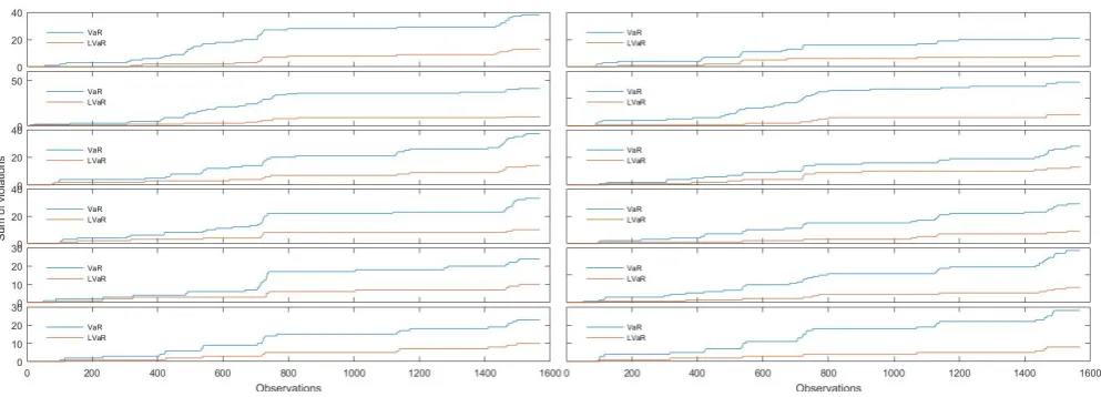
industry is testing the independence by visual inspection of the cluster of the exceptions
(see Acerbi and Szekely (2014), section 1). We conduct an empirical analysis with the
available data which shows that ΛV aR clusters the exceptions considerably less than
V aR and suggests a higher level of independence of the ΛV aR exceptions (as shown
in Figure (1)). The reason behind might be that ΛV aR is recalculated at each time t
incorporating the recent market movements and, in this way, it may avoid sequential
violations. However, in order to have a complete assessment of the accuracy of a risk
on the immediate extension of theV aRframework since the exceptions are not identically
[image:9.595.62.559.154.333.2]distributed. This requires a more complex analysis that we leave for a future study.
Figure 1: Time evolution of the sum of violations for 1%V aRand ΛV aR. The table shows the evolution over the global financial crisis of the sum of violations of the 1%V aRand the increasing ΛV aR model.
The first theoretical proposal for the backtesting of V aR is given by Kupiec (1995),
where the author considers the following null and alternative hypothesis:
H0K :λt ≤(=)λ0 for any t
H1K :λt > λ0 for some t and equal otherwise
(6)
whereλ0 is theV aRconfidence level. TheV aRat levelλ0 is accepted if the frequency
of the exceptions does not exceed the confidence level λ0 for any t.
Recently, Hitaj, Mateus, and Peri (2015) have proposed a backtesting method for
ΛV aR by adapting the classical Kupiec test for V aR. They consider the following null
and alternative hypothesis:
H0K :λt≤max(Λ) for any t
H1K :λt>max(Λ) for some t and equal otherwise
Substantially, ΛV aR is accepted if the frequency of violations is less than max(Λ). This
is an unilateral hypothesis test that can be conducted by using the same log-likelihood
ratio and critical value of the V aR test. This approach permits to verify if the coverage
objective given by the Λ maximum has been reached, however, it does not allow to
evaluate the accuracy of ΛV aR at any timet.
Indeed, if the ΛV aR model is correct, at time t we should be expecting that the hit
sequence assumes value 1 with probability
λ0t = Λt(−ΛV aRt) (8)
and 0 with probability 1−λ0
t. This intuition is correct if both Λt and Pt are continuous.
In case this does not occur, we have λ0t =Pt(−ΛV aRt).
As a consequence, the random variables It of the violations for ΛV aR are not
iden-tically distributed, which implies that usual likelihood backtesting framework (POF by
Kupiec 1995 , TUFF by Christoffersen 2010 etc.) cannot be directly applied.
Hence, if ΛV aRis correct, the null hypothesis should be:
H0 :λt=λ0t for any t (9)
while the alternative hypothesis, either:
in case of a bilateral test, or:
H1 :λt> λ0t for some t and equal otherwise (11)
in case of an unilateral test where we reject in presence of risk under-estimation.
The null hypothesis in (9) allows to evaluate if ΛV aRguarantees the level of coverage
predicted by theλ0
t parameter. In this way, we are able to assess the correctness of ΛV aR
more precisely than Hitaj, Mateus, and Peri (2015). Notice that a rejection of HK
0 in (7)
implies a rejection of H0 in (9). Observe also that these hypothesis tests are also valid
for V aR at confidence level λ0 by fixing λ0
t =λ0 for any t.
In order to test the accuracy of the ΛV aR model, we propose three test statistics.
The distribution of the first two test statistics is obtained by exploiting simple results of
probability theory. In particular, the second test provides an asymptotic result, hence it
is more suitable for larger samples of observations (i.e. time horizon larger than 500).
We propose also a third test that is more useful to check if ΛV aRhas been estimated
with the correct distribution function, Pt. Here, the correctness of the null hypothesis is
evaluated by a simulation exercise.
We suggest that the first two tests are used for an initial validation of the ΛV aRmodel,
while the third test is used as second step for selecting the best choice of estimation for
3.1
Test 1
We set the null and the alternative hypothesis as in (9) and (11), respectively. We
construct this first test by defining the test statisticZ1 equal to the number of violations
over the time horizon T, as follows:
Z1 :=
T
X
t=1
It (12)
The distribution of Z1 is obtained by applying classical results of probability theory. If
the violations It independently occurs, the sum of independent Bernoulli with different
mean follows a Poisson Binomial distribution (λt), thus we have that under H0:
Z1 ∼Poiss.Bin({λ0t}). (13)
This test is in principle a bilateral test, with critical region: C = z1 :z1 < qZ1(
α
2) ∪
z1 :z1 ≥qZ1(1−
α
2) , where α denotes the significance level of the test (i.e. 1 type
error) and qZ1 is the quantile of the Z1 distribution under H0, i.e. PZ1. However, in the
backtesting practice, this test can be treated as unilateral, where the critical region is
given by:
CZ1 ={z1 :z1 ≥qZ1(1−α)}={z1 :PZ1(z1)>1−α} (14)
Indeed, the probability that z1 falls in the left side of the critical region C is null, since
qZ1(
α
2) is zero any time the following relation is satisfied: (1−max(λt))
T > α/2. This is
typical for usual test significance levels (α= 10% or lower), usual time horizon T = 250
This test represents an extension of the traffic light approach by Basel Committee on
Banking Supervision (1996) to ΛV aRwith two bands instead of three. In particular, for
V aR at confidence level λ0, under H0 we have:
Z1 ∼Bin(T, λ0)
that is Z1 follows a Binomial distribution. In the empirical analysis we fix α= 10% and
we compare the results with V aR.
3.2
Test 2
We propose a second test statistic that is founded on a result of probability theory known
as Lyapunov theorem. We set the null and the alternative hypothesis as in (9) and (10),
respectively. We propose another test statistic defined as follows:
Z2 :=
PT
t=1(It−λ0t)
q PT
1 λ 0
t(1−λ0t)
(15)
Under H0, Z2 is asymptotically distributed as a Standard Normal, formally:
Z2
d
−
→N(0,1) (16)
This result follows from the application of Lemma 2 and the Lyapunov’s theorem (see
Appendix for details).
realization z2 of the test statistic stays in the following critical region:
CZ2 :=
n
z2 :z2(x)< qZ2
α
2
o
∪nz2 :z2(x)> qZ2
1− α
2
o
(17)
whereαis the significance level of the test, andqZ2 is the quantile function of the Standard
Normal distribution PZ2.
Also for this test, in the empirical analysis, we fix α = 10% and we compare the
results with V aR.
3.3
Test 3
The third test is inspired by Acerbi and Szekely (2014) and focused on another aspect.
The aim of this test is to directly verify if ΛV aR has been estimated under the correct
assumption on the distributionPtof the returns. To this purpose we build a test statistic,
Z3, and we proceed by simulating its distribution using the same assumption as for the
asset return distribution in the risk measure computation.
We set the null and the alternative hypothesis as in (9) and (11), respectively, and we
define Z3 as follows:
Z3 :=
1
T
T
X
t=1
(λ0t −It) =
1
T
T
X
t=1
λ0t − 1 T
T
X
t=1
It (18)
We observe that under H0, we have E[Z3] = 0, while under H1, E[Z3]<0 for ΛV aR
(see Proposition (3) in Appendix). So, if the model is correct the realized value z3
is expected to be zero. On the other hand, a negative z3 is a signal that the model
Under H0 the distribution of Z3 depends on the assumption for the distribution Pt of
the asset returns. Hence, we perform the test by simulating M scenarios of the
distribu-tion Pt of the returns at each time t, with t = 1, . . . , T. In this way, we obtain at time
T the distribution PZ3 of the test statistic under H0. In order to construct the critical
region we need to study the behavior of PZ3 when the distribution of the returns changes
fromP to F. Let us compute PZ3:
PZ3 =P(Z3 ≤z) =P
1
T
T
X
t=1
(λ0t −It)≤z
!
=P
T
X
t=1
(−It)≤zT − T
X
t=1 λ0t
!
=P
T
X
t=1
It≥ −zT + T
X
t=1 λ0t
!
where PT
t=1It is distributed as a Binomial Poisson of parameter {λt}. We observe that
PZ3 is an increasing function of {λt} (i.e. PZ3 shifts to left when λt increases). As a
consequence, given a significance level α, we reject the null hypothesis when the p-value
p=PZ3(z) is smaller than α.
In the empirical analysis we conduct M = 10000 simulations using the same
assump-tions on the asset return distribution as for the risk measures computation. We set the
test significance level α at 10%.
This test allows to verify how the choice of the asset return distribution influences
the risk coverage capacity of ΛV aR, that, instead, is not directly assessed by Test 1 and
Test 2. Hence, the best use of Test 3 is comparing the results between the same kind
of ΛV aRmodels, but estimated with different assumptions on the P&L distribution (i.e.
The limit of this test is that requires a massive storage of information, since at time
T we need all the predictive distributions Pt of the returns for t= 1, . . . , T.
4
Empirical analysis
In this section, we provide an empirical analysis of the backtesting methods of ΛV aR
that we have defined in Section (3). We applied the tests to a slightly different version of
the 1%−ΛV aRmodels proposed in Hitaj, Mateus, and Peri (2015) and to the 1%−V aR
model. We compare the backtesting results with the Kupiec-type test proposed in Hitaj,
Mateus, and Peri (2015) for ΛV aR and with the classical Kupiec’s test for V aR.
We refer to the same dataset as in Hitaj, Mateus, and Peri (2015), consisting in daily
data of 12 stocks quoted in different countries along different time windows throughout
the global financial crisis (specifically, from January 2005 to December 2011). These
comprise the stocks of Citigroup Inc. (C UN Equity) and Microsoft Corporation (MSFT
UW Equity) for the United States, Royal Bank of Scotland Group PLC (RBS LN Equity)
and Unilever PLC (ULVR LN Equity) for the United Kingdom, Volkswagen AG (VOW3
GY Equity) and Deutsche Bank AG (DBK GY Equity) for Germany, Total SA (FP FP
Equity) and BNP Paribas SA (BNP FP Equity) for France, Banco Santander SA (SAN
SQ Equity) and Telefonica SA (TEF SQ Equity) for Spain, and Intesa Sanpaolo SPA
(ISP IM Equity) and Enel SPA (ENEL IM Equity) for Italy. The market benchmarks
for the ΛV aRcomputation have been chosen among the market indexes with the highest
volume of exchanges; these are S&P500, FTSE 100, and EURO STOXX 50.
distri-bution of the asset returns. We consider the classical Historical and Normal simulation
approach and we add robustness to the analysis by implementing GARCH models with
t-student increments and the Extreme Value Theory (EVT) method based on the
gen-eralised Pareto distribution (we remand to McNeil, Frey, and Embrechts (2005) for a
review on this method). The estimation of the parameters is based on 250 days of
ob-servations for the Historical and Normal assumption, while 500 days are considered for
the GARCH model. For the Extreme Value Theory method, we implement an automatic
routine to identify the threshold in the different time windows.
The backtesting exercise is conducted comparing the realized ex-post daily returns
with the daily V aRand ΛV aRestimates of the 12 stocks over the time period of 1 year.
In particular, we split the analysis into six different 2-year time windows (250 days for
the risk measure computation and 1 year for the backtesting).
4.1
Results
4.1.1 Violations and Kupiec test
We first report the results of the violations and the Kupiec test for the V aR model and
the Kupiec-type test adapted by Hitaj, Mateus, and Peri (2015) for the ΛV aR model.
We compute the average number of violations and acceptance rate over all the assets and
different time horizon T. The results presented, hereafter, in Table (1) are under the
Average number of violations Kupiec-Test
2006 2007 2008 2009 2010 2011 2006 2007 2008 2009 2010 2011
VaR 1% 3.42 5.33 11.58 0.75 3.08 6.83 100 % 83 % 0 % 100 % 92 % 50 %
3.42 5.33 11.58 0.75 3.08 6.83 100% 83% 0% 100% 92% 50%
ΛV aR1%(decr)
(VaR 5%) 2.25 3.67 7.00 0.67 2.00 4.25 100 % 83 % 42 % 100 % 100 % 83 %
(VaR 1%) 2.17 2.33 5.75 0.67 1.58 4.00 100 % 83 % 67 % 100 % 100 % 83 %
2.21 3.00 6.38 0.67 1.79 4.13 100 % 83 % 54 % 100 % 100 % 83 %
ΛV aR1%(incr)
(VaR 5%) 1.17 1.00 3.92 0.42 0.92 2.75 100 % 100 % 100 % 100 % 100 % 100 %
(VaR 1%) 1.17 1.08 3.92 0.42 1.00 2.75 100 % 100 % 100 % 100 % 100 % 100 %
[image:18.595.77.528.102.280.2]1.17 1.04 3.92 0.42 0.96 2.75 100 % 100 % 100 % 100 % 100 % 100 %
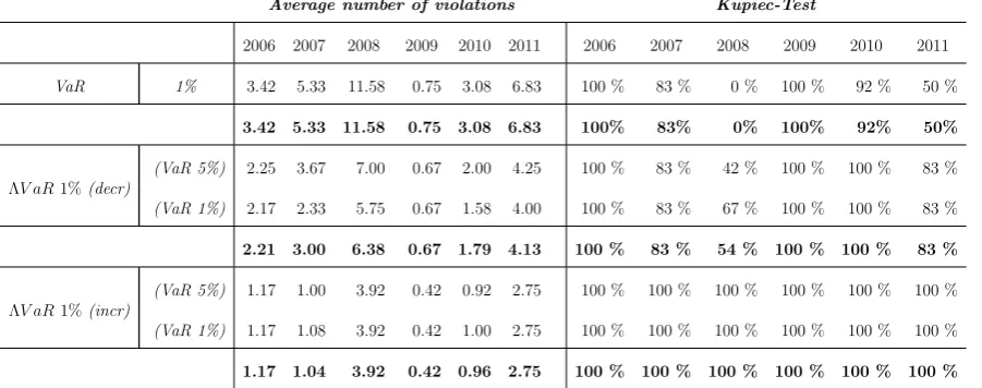
Table 1: Time evolution of the average number of violations and Kupiec test under the Historical distribution assumption. The table shows the evolution over the global financial crisis of the average number of violations and the percentage of Kupiec acceptance, aggregated at the level of 1%V aR, as well as the increasing and decreasing ΛV aRmodels.
As expected and already pointed out in Hitaj, Mateus, and Peri (2015) the average
number of violations of 1%V aRis bigger than the one of ΛV aR, in particular if compared
with the increasing models. In fact 1% V aR shows a drastic increase in the average
number of violations, moving from 3.42 in 2006 to 11.58 in 2008. On the other hand, the
increasing ΛV aR models register an average number of violations of around 1.17 during
2006 and retain the number at around 3.92 in the 2008 crisis.
This result was expected since the Λ function has been built with maxxΛt(x) = 0.01,
which implies that ΛV aR is always greater or equal than 1% V aR, so that, losses not
covered by the first are also not covered by the latter. This implies that ΛV aR performs
always better than 1% V aR by using an unilateral Kupiec-type test, since this kind of
test does not capture the variability of the Λ function that is the essential feature of
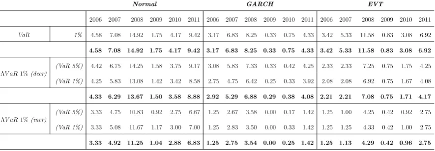
The violations trend is the same also under the other distribution’s assumptions taken
in exam as shown in Table (2).
Normal GARCH EVT
2006 2007 2008 2009 2010 2011 2006 2007 2008 2009 2010 2011 2006 2007 2008 2009 2010 2011
VaR 1% 4.58 7.08 14.92 1.75 4.17 9.42 3.17 6.83 8.25 0.33 0.75 4.33 3.42 5.33 11.58 0.83 3.08 6.92
4.58 7.08 14.92 1.75 4.17 9.42 3.17 6.83 8.25 0.33 0.75 4.33 3.42 5.33 11.58 0.83 3.08 6.92
ΛV aR1%(decr)
(VaR 5%) 4.42 6.75 14.25 1.58 3.75 9.17 3.08 5.83 7.33 0.33 0.42 4.25 2.33 2.33 7.25 0.75 1.75 4.25
(VaR 1%) 4.25 5.83 13.08 1.42 3.42 8.58 2.75 4.75 6.42 0.25 0.33 3.92 2.08 2.08 6.92 0.75 1.67 4.08
4.33 6.29 13.67 1.50 3.58 8.88 2.92 5.29 6.88 0.29 0.38 4.08 2.21 2.21 7.08 0.75 1.71 4.17
ΛV aR1%(incr)
(VaR 5%) 3.33 4.75 10.83 0.92 2.75 6.67 1.25 2.67 3.58 0.00 0.17 1.42 1.25 1.00 4.25 0.42 0.92 2.75
(VaR 1%) 3.33 5.08 11.67 1.17 3.00 7.00 1.25 2.83 3.50 0.00 0.33 1.42 1.25 1.25 4.33 0.42 1.00 2.75
[image:19.595.79.522.167.321.2]3.33 4.92 11.25 1.04 2.88 6.83 1.25 2.75 3.54 0.00 0.25 1.42 1.25 1.13 4.29 0.42 0.96 2.75
Table 2: Time evolution of the average number of violations under the Normal, GARCH and EVT model. The table shows the evolution over the global financial crisis of the average number of violations aggregated at the level of 1%V aR, as well as the increasing and decreasing ΛV aR models.
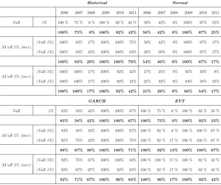
4.1.2 Test 1 and Test 2: comparison of V aR and ΛV aR risk coverage
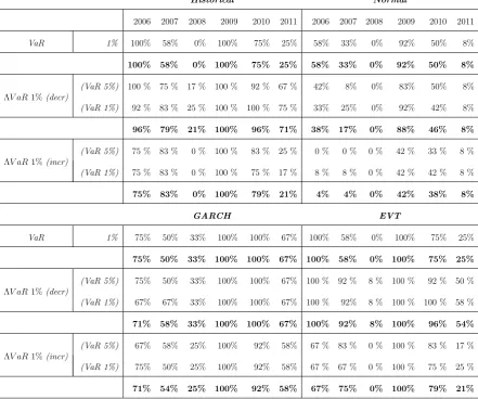
In Table (3) and (4) we show the results of Test 1 and 2 proposed in Section (3) for
ΛV aR. The results here presented are under different assumptions of the distribution of
Historical Normal
2006 2007 2008 2009 2010 2011 2006 2007 2008 2009 2010 2011
VaR 1% 100% 58% 0% 100% 75% 25% 58% 33% 0% 92% 50% 8%
100% 58% 0% 100% 75% 25% 58% 33% 0% 92% 50% 8%
ΛV aR1%(decr)
(VaR 5%) 100 % 75 % 17 % 100 % 92 % 67 % 42% 8% 0% 83% 50% 8%
(VaR 1%) 92 % 83 % 25 % 100 % 100 % 75 % 33% 25% 0% 92% 42% 8%
96% 79% 21% 100% 96% 71% 38% 17% 0% 88% 46% 8%
ΛV aR1%(incr)
(VaR 5%) 75 % 83 % 0 % 100 % 83 % 25 % 0 % 0 % 0 % 42 % 33 % 8 %
(VaR 1%) 75 % 83 % 0 % 100 % 75 % 17 % 8 % 8 % 0 % 42 % 42 % 8 %
75% 83% 0% 100% 79% 21% 4% 4% 0% 42% 38% 8%
GARCH EVT
VaR 1% 75% 50% 33% 100% 100% 67% 100% 58% 0% 100% 75% 25%
75% 50% 33% 100% 100% 67% 100% 58% 0% 100% 75% 25%
ΛV aR1%(decr)
(VaR 5%) 75% 50% 33% 100% 100% 67% 100 % 92 % 8 % 100 % 92 % 50 %
(VaR 1%) 67% 67% 33% 100% 100% 67% 100 % 92% 8 % 100 % 100 % 58 %
71% 58% 33% 100% 100% 67% 100% 92% 8% 100% 96% 54%
ΛV aR1%(incr)
(VaR 5%) 67% 58% 25% 100% 92% 58% 67 % 83 % 0 % 100 % 83 % 17 %
(VaR 1%) 75% 50% 25% 100% 92% 58% 67 % 67 % 0 % 100 % 75 % 25 %
[image:20.595.78.520.105.473.2]71% 54% 25% 100% 92% 58% 67% 75% 0% 100% 79% 21%
Historical Normal
2006 2007 2008 2009 2010 2011 2006 2007 2008 2009 2010 2011
VaR 1% 100 % 75 % 0 % 100 % 92 % 42 % 58% 42% 0% 100% 67% 25%
100% 75% 0% 100% 92% 42% 58% 42% 0% 100% 67% 25%
ΛV aR1%(decr)
(VaR 5%) 100% 83% 17% 100% 100% 75% 58% 42% 0% 100% 67% 17%
(VaR 1%) 100% 83% 42% 100% 100% 83% 50% 50% 0% 100% 67% 17%
100% 83% 29% 100% 100% 79% 54% 46% 0% 100% 67% 17%
ΛV aR1%(incr)
(VaR 5%) 100% 100% 17% 100% 92% 42% 17% 25% 0% 92% 50% 8%
(VaR 1%) 100% 100% 17% 100% 92% 42% 25% 33% 0% 83% 58% 25%
100% 100% 17% 100% 92% 42% 21% 29% 0% 88% 54% 17%
GARCH EVT
VaR 1% 83% 58% 42% 100% 100% 67% 100 % 75 % 0 % 100 % 92 % 33 %
83% 58% 42% 100% 100% 67% 100% 75% 0% 100% 92% 33%
ΛV aR1%(decr)
(VaR 5%) 83% 58% 33% 100% 100% 67% 100 % 92 % 8 % 100 % 100 % 67 %
(VaR 1%) 92% 75% 42% 100% 100% 75% 100 % 92 % 17 % 100 % 100 % 67 %
88% 67% 38% 100% 100% 71% 100% 92% 13% 100% 100% 67%
ΛV aR1%(incr)
(VaR 5%) 92% 75% 67% 100% 100% 83% 100 % 100 % 17 % 100 % 92 % 42 %
(VaR 1%) 92% 67% 67% 100% 92% 83% 100 % 92 % 17 % 100 % 92 % 42 %
[image:21.595.78.520.99.467.2]92% 71% 67% 100% 96% 83% 100% 96% 17% 100% 92% 42%
Table 4: Time evolutions of Test 2 for the ΛV aR models under different assumptions of the P&L distribution. The table shows the evolution over the global financial crisis of the acceptance rates, aggregated at the level of the ΛV aRmodels (minxΛ(x) = 0.5%) calculated using the Historical, Normal, GARCH and EVT assumption of the P&L distribution.
We first notice that the acceptance rate of these tests is lower than the unilateral
Kupiec test in Hitaj, Mateus, and Peri (2015). This is due to the particular construction
of the Kupiec test. Indeed, this test is useful to assess if the ΛV aR model guarantees
an acceptable coverage given by max(Λ), but cannot capture the daily variations of the
confidence levelλ0t of ΛV aR. Thus, it cannot be used to evaluate the real coverage offered
to better evaluate if the flexibility introduced by the Λ function helps to detect adverse
scenario and put aside a more adequate amount of capital.
If we compare the tests results, we observe that for all the models Test 2 provides
higher acceptance rates in respect to Test 1. This may be due to the fact that Test 1
returns more precise results with smaller number of observations and also to its unilateral
nature that attributes the highest weight to the violations.
With the exception of the normal estimator, the ΛV aR models result often more
accurate than 1% V aR, confirming the outcomes in Hitaj, Mateus, and Peri (2015).
This means that the highest flexibility of ΛV aR contributes to the highest coverage,
especially when it is computed with distributions that better capture the tail behaviour.
In our tests, the decreasing ΛV aRmodels seem to be more accurate, in contrast with the
results of the Kupiec test. We think this is a consequence of a lower power of these tests
for the decreasing ΛV aR models. We remand the analysis of the test power for further
research since it would complicate this study without adding significant value.
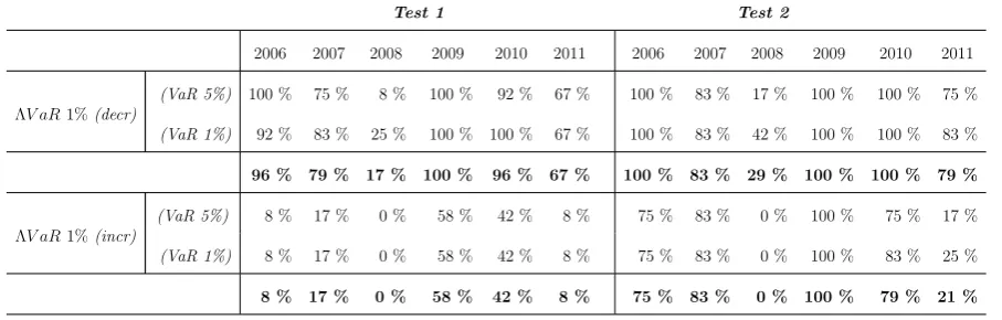
4.1.3 The choice of the Λ minimum
During the analysis of the results, Test 1 and Test 2 have pointed out an issue of estimation
in the ΛV aR models proposed by Hitaj, Mateus, and Peri (2015). In particular, the
authors do not discuss in details the choice of the Λ minimum, minxΛ(x), that seems to
be set equal to 0.1% after empirical experimentations. In addition, the extended Kupiec
test proposed by the authors could not identify the impact of this choice.
When we have run for the first time Test 1 and 2 using the choice of Hitaj, Mateus,
presented the highest rejection rate, even if they had the smallest number of infractions,
as shown by Table (5).
Test 1 Test 2
2006 2007 2008 2009 2010 2011 2006 2007 2008 2009 2010 2011
ΛV aR1%(decr)
(VaR 5%) 100 % 75 % 8 % 100 % 92 % 67 % 100 % 83 % 17 % 100 % 100 % 75 %
(VaR 1%) 92 % 83 % 25 % 100 % 100 % 67 % 100 % 83 % 42 % 100 % 100 % 83 %
96 % 79 % 17 % 100 % 96 % 67 % 100 % 83 % 29 % 100 % 100 % 79 %
ΛV aR1%(incr)
(VaR 5%) 8 % 17 % 0 % 58 % 42 % 8 % 75 % 83 % 0 % 100 % 75 % 17 %
(VaR 1%) 8 % 17 % 0 % 58 % 42 % 8 % 75 % 83 % 0 % 100 % 83 % 25 %
[image:23.595.74.528.167.312.2]8 % 17 % 0 % 58 % 42 % 8 % 75 % 83 % 0 % 100 % 79 % 21 %
Table 5: Time evolutions of Test 1 and Test 2 for the ΛV aRmodels with minxΛ(x) = 0.1% under the Historical distribution assumption. The table shows the evolution over the global financial crisis of the acceptance rates, aggregated at the level of the ΛV aR models with minxΛ(x) = 0.1%.
Thus, we have studied how the probability of infraction λt evolves in the different
ΛV aR models and we have observed that in most of the cases it obtains the minimal
value. This happens especially during crisis periods, when the cumulative distribution
function of the assets shifts on the left and intersects the Λ function at the minimum
level. In such a case, the choice of the Λ minimum is relevant and also a critical issue.
From our point of view, the Λ minimum should provide the probability to lose more
than the worst case event (i.e. benchmarks’ minimum, π1 = minxt,j) over the time
window observations (i.e. 250 in our case). If we consider all the events equally probable,
the selection of the Λ minimum should be greater than 1/T over T observations. Thus,
we propose to compute the ΛV aR models by fixing the Λ minimum equal to 0.5%, i.e.
minxΛ(x) = 0.005, since the probability of an event over 250 past realizations is 0.4%.
Table (3) and (4). The number of infractions does not change in any period under
consid-eration, while the acceptance rate of the increasing ΛV aR models drastically increases,
validating our choice. Clearly, this new setting does not affect the decreasing ΛV aR
models. Anyway, the choice of the Λ minimum can be refined considering more precise
evaluation of the probability of the worst case event, but this is beyond the objective of
this paper.
4.1.4 Test 3: comparison of ΛV aRs with different distribution estimations
As anticipated in Section (3), the best use of Test 3 is the comparison of the accuracy of
the risk measures computed with different estimations of asset return distribution. We
compute the time evolution of the acceptance rate aggregated at the level of the increasing
and decreasing ΛV aR models. We repeat the analysis changing the assumption on the
asset return distribution: specifically, Historical, Monte Carlo Normal, GARCH and EVT
Historical Normal
2006 2007 2008 2009 2010 2011 2006 2007 2008 2009 2010 2011
VaR 1% 50% 33% 0% 100% 58% 25% 58% 33% 0% 92% 50% 8%
50% 33% 0% 100% 58% 25% 58% 33% 0% 92% 50% 8%
ΛV aR1%(decr)
(VaR 5%) 50% 33% 0% 100% 67% 17% 58% 42% 0% 92% 58% 17%
(VaR 1%) 58% 50% 8% 100% 67% 8% 50% 33% 0% 92% 58% 25%
54% 42% 4% 100% 67% 13% 54% 38% 0% 92% 58% 21%
ΛV aR1%(incr)
(VaR 5%) 8% 17% 0% 58% 42% 0% 17% 17% 0% 92% 50% 8%
(VaR 1%) 8% 17% 0% 58% 42% 8% 33% 8% 0% 83% 50% 17%
8% 17% 0% 58% 42% 4% 25% 13% 0% 88% 50% 13%
GARCH EVT
VaR 1% 75% 58% 33% 100% 100% 67% 50 % 33 % 0 % 100 % 58 % 25 %
75% 58% 33% 100% 100% 67% 50% 33% 0% 100% 58% 25%
ΛV aR1%(decr)
(VaR 5%) 75% 58% 33% 100% 100% 67% 67 % 58 % 0 % 92 % 58 % 42 %
(VaR 1%) 92% 67% 33% 100% 100% 75% 67 % 58 % 0 % 92 % 58 % 33 %
83% 63% 33% 100% 100% 71% 67% 58% 0% 92% 58% 38%
ΛV aR1%(incr)
(VaR 5%) 83% 67% 67% 100% 100% 83% 17 % 25 % 8 % 58 % 42 % 0 %
(VaR 1%) 83% 58% 67% 100% 92% 83% 17 % 33 % 0 % 58 % 42 % 8 %
[image:25.595.79.520.101.485.2]83% 63% 67% 100% 96% 83% 17% 29% 4% 58% 42% 4%
Table 6: Time evolutions of Test 3 for the ΛV aR models under different assumptions of the P&L distribution. The table shows the evolution over the global financial crisis of the acceptance rates, aggregated at the level of the ΛV aRmodels (minxΛ(x) = 0.5%) calculated using the Historical, Normal, GARCH and EVT assumption of the P&L distribution.
The results show that the GARCH assumption on the returns guarantees the highest
accuracy in terms of average acceptance rate. Moreover, we notice here that the Historical
and the EVT estimators of the increasing ΛV aR often underperform the Normal one, in
contrast with the previous tests. These outcomes are quite reasonable since this third
distributions having cut-off tails (as the Historical) or based on a small range of values (as
the EVT). However, such a preference for the Normal distribution is completely reversed
by the other tests which privilege the assumption of distributions which rely more on tail
events and not on the full shape of the distribution.
5
Conclusions
A new risk measure sensitive to tail risk, ΛV aR, has been recently introduced. However,
anad hoc study on its backtesting has not been conducted in literature so far. The main
issue for the ΛV aRbacktesting is that the probability of a violation is not constant, but
may change at any time and for any asset. This consideration implies that the
Kupiec-type backtesting framework, proposed by Hitaj, Mateus, and Peri (2015), fails to keep
into account the effective predictive capacity of ΛV aR as introduced by the Λ function.
We propose three backtesting methodologies for ΛV aR and we asses the accuracy of
the new risk measure from different points of view. Test 1 and Test 2 are based on results
of probability theory and allow for a straightforward application. Test 3 is performed by
simulations and allows for more accurate comparison of ΛV aR models estimated under
different assumptions on the P&L distribution.
The validity of our backtesting proposals is confirmed by the results of the empirical
analysis. In fact, this study shows that ΛV aR models perform better than 1 % V aR,
confirming the findings in Hitaj, Mateus, and Peri (2015). In addition, ΛV aRcomputed
with the GARCH model of returns has the highest level of coverage. This outcome
explain better the real asset return behavior and allow for a more accurate risk coverage.
Moreover, our backtesting methods denote higher precision than the Kupiec-type test
proposed by Hitaj, Mateus, and Peri (2015) since they have been able to detect an
estimation issue of ΛV aR computed with a lower bound of 0.1% as in the former study.
Suggestions for future research include the study of the test power that would permit
a more accurate comparison among these backtesting proposals.
Appendix
We recall hereafter the Lyapunov Theorem that is a result of probability theory based
on the application of the central limit theorem to random variables that are independent
but not identically distributed (see Lyapunov 1954).
Theorem 1 (Lyapunov) SupposeX1, X2, ...is a sequence of independent random
vari-ables, each with finite expected value µt and variance σ2t. Define
s2n =
T
X
t=1 σt2
If for some δ >0, the “Lyapunov’s condition”
lim
n→∞ 1
s2+T δ
T
X
t=1
E|Xt−µt|2+δ
= 0
is satisfied, then the following convergence in distribution holds as T goes to infinity:
1
sT T
X
t=1
(Xt−µt) d
−
In the following lemma we show that the “Lyapunov’s condition” is satisfied when
s2
T =
PT
1 λt(1−λt) and µt=λt.
Lemma 2 If{It}is a sequence of independent random variables distributed as a Bernoulli
with parameters {λt}t and inftλt=λm >0, then
lim
T→∞ 1
s2+T δ
T
X
t=1
E[|It−λt|2+δ] = 0
with s2
T =
PT
1 λt(1−λt).
Proof. We observe that:
E[|It−λt|2+δ] = (1−λt)λ2+t δ+λt(1−λt)2+δ
=λt(1−λt) λt1+δ+ (1−λt)1+δ
≤λt(1−λt)≤
1 4.
On the other hand we have
s2+T δ =
T
X
1
λt(1−λt)
!1+δ2
≥
T
X
1
λm(1−λm)
!1+2δ
= (T λm(1−λm))
1+δ
2 .
We can thus conclude that
PT
t=1E[|It−λt| 2+δ]
s2+T δ ≤
T
4 (T λm(1−λm))1+ δ
2
→0
as T → ∞.
The following proposition shows theoretical implications on the Z3 test statistic in
Proposition 3 Under the test hypothesis H0 as in (9) and H1 as in (11) we have:
1. EH0[Z3] = 0
2. EH1[Z3]<0.
Proof. It is enough to notice that under H0, It ∼B(λ0t) so that EH0[It−λ
0
t] = 0, which
implies
EH0[Z3] =
1
T X
EH0[λ
0
t −It] = 0.
In a similar way, under H1, sinceIt∼B(λt) with λt> λ0t, we obtain that EH1[Z3]<0.
References
Acerbi, C., and B. Szekely. 2014. ”Back-testing Expected Shortfall.” Risk 27 (11): 76-81.
Berkowitz, J., P. Christoffersen, and D. Pelletier. 2011. ”Evaluating Value-at-Risk Models
with Desk-Level Data.” Management Science 57: 2213-2227.
Basel Committee on Banking Supervision. 1996. ”Supervisory Framework for the Use of
Backtesting in Conjunction with the Internal Models Approach to Market Risk Capital
Requirements.” Bank for International Settlements.
Basel Committee on Banking Supervision. 2013. ”Fundamental Review of the Trading
Book.” 2nd consultative document. Bank for International Settlements.
Economics Discussion Series. Divisions of Research & Statistics and Monetary Affairs,
Federal Reserve Board, Washington D.C.
Christoffersen, P. 2010. ”Encyclopedia of Quantitative Finance - Backtesting.” Wiley
Online Library.
Frittelli, M., M. Maggis, and I. Peri. 2014. ”Risk Measures on and Value at Risk with
Probability/Loss Function.” Mathematical Finance 24 (3): 442-463.
Hitaj, A., C. Mateus, and I. Peri. 2015. ”Lambda Value at Risk and
Regula-tory Capital: a Dynamic Approach to Tail Risk.” Working paper available at
http://ssrn.com/abstract=2932475.
Kupiec, P. 1995. ”Techniques for Verifying the Accuracy of Risk Measurement Models.”
Journal of Derivatives 3 (2): 73-84.
Lyapunov, A. M. 1954. ”Collected Works 1.” Moscow-Leningrad, 157-176.
McNeil, A. J., R. Frey, and P. Embrechts. 2005. ”Quantitative Risk Management:
Con-cepts, Techniques and Tools.” Princeton University Press, 3 Market Place, Woodstock,