https://doi.org/10.5194/gmd-10-3913-2017 © Author(s) 2017. This work is distributed under the Creative Commons Attribution 4.0 License.
GLOFRIM v1.0 – A globally applicable computational framework
for integrated hydrological–hydrodynamic modelling
Jannis M. Hoch1,2, Jeffrey C. Neal3, Fedor Baart2, Rens van Beek1, Hessel C. Winsemius2,4, Paul D. Bates3, and Marc F. P. Bierkens1,2
1Department of Physical Geography, Utrecht University, P.O. Box 80115, 3508 TC Utrecht, the Netherlands 2Deltares, P.O. Box 177, 2600 MH Delft, the Netherlands
3School of Geographical Sciences, University of Bristol, University Road, Bristol, BS8 1SS, UK
4Institute for Environmental Studies, VU University, De Boelelaan 1087, 1081 HV, Amsterdam, the Netherlands Correspondence to:Jannis M. Hoch ([email protected])
Received: 16 June 2017 – Discussion started: 19 June 2017
Revised: 15 September 2017 – Accepted: 25 September 2017 – Published: 27 October 2017
Abstract. We here present GLOFRIM, a globally applica-ble computational framework for integrated hydrological– hydrodynamic modelling. GLOFRIM facilitates spatially ex-plicit coupling of hydrodynamic and hydrologic models and caters for an ensemble of models to be coupled. It currently encompasses the global hydrological model PCR-GLOBWB as well as the hydrodynamic models Delft3D Flexible Mesh (DFM; solving the full shwater equations and allow-ing for spatially flexible meshallow-ing) and LISFLOOD-FP (LFP; solving the local inertia equations and running on regular grids). The main advantages of the framework are its open and free access, its global applicability, its versatility, and its extensibility with other hydrological or hydrodynamic models. Before applying GLOFRIM to an actual test case, we benchmarked both DFM and LFP for a synthetic test case. Results show that for sub-critical flow conditions, dis-charge response to the same input signal is near-identical for both models, which agrees with previous studies. We subse-quently applied the framework to the Amazon River basin to not only test the framework thoroughly, but also to per-form a first-ever benchmark of flexible and regular grids on a large-scale. Both DFM and LFP produce comparable results in terms of simulated discharge with LFP exhibiting slightly higher accuracy as expressed by a Kling–Gupta efficiency of 0.82 compared to 0.76 for DFM. However, benchmark-ing inundation extent between DFM and LFP over the en-tire study area, a critical success index of 0.46 was obtained, indicating that the models disagree as often as they agree. Differences between models in both simulated discharge and
inundation extent are to a large extent attributable to the grid-ding techniques employed. In fact, the results show that both the numerical scheme of the inundation model and the grid-ding technique can contribute to deviations in simulated in-undation extent as we control for model forcing and bound-ary conditions. This study shows that the presented computa-tional framework is robust and widely applicable. GLOFRIM is designed as open access and easily extendable, and thus we hope that other large-scale hydrological and hydrody-namic models will be added. Eventually, more locally rel-evant processes would be captured and more robust model inter-comparison, benchmarking, and ensemble simulations of flood hazard on a large scale would be allowed for.
1 Introduction
neighbouring river basins (Jongman et al., 2014), it is vital that flood hazard models can simulate the relevant processes over large domains. Applying such large-scale models has the additional advantage of facilitating the identification of risk hotspots and providing critical insight into data-scarce areas (Ward et al., 2015). In fact, there are already a num-ber of global-scale inundation models available (Dottori et al., 2016; Pappenberger et al., 2012; Sampson et al., 2015; Winsemius et al., 2013; Yamazaki et al., 2011), differing in their process descriptions and computational engine. While some approaches derive flood hazard from a coarse-scale hy-drological model and subsequent downscaling, others force fine-scale hydrodynamic models with globally regionalized discharge data. A first inter-comparison of global flood haz-ard models by Trigg et al. (2016) for the African continent, however, revealed that they agree for only 30–40 % of ag-gregated flood extent, thus indicating that the representative-ness of local flood risk estimates may depend strongly on the computational engine opted for as well as on the model forcing applied. Identifying the exact reasons for model dis-agreement was impossible due to the diversity of methods and lack of a systematic approach to the inter-comparison where individual aspects of the modelling frameworks could be isolated.
Employing a global hydrological model such as PCR-GLOBWB (van Beek et al., 2011; van Beek and Bierkens, 2008), WaterGAP (Alcamo et al., 1997; Döll et al., 2003) or VIC (Liang et al., 1994; Wood et al., 1992) has the benefit of providing spatially distributed surface runoff and routed dis-charge simulations, thereby facilitating direct forcing for spa-tially distributed inundation models. In addition, these mod-els are usually forced by global meteorological data, hence diminishing the dependency on observed data as well as al-lowing for easier implementation of future climate scenar-ios. However, the routing schemes currently implemented in large-scale hydrological models can generally be described as simplistic as they are based on gridded drainage networks at a coarse spatial resolution, with the currently finest spa-tial resolution of global hydrological models being 5 arcmin or around 10 km×10 km at the Equator (Bierkens, 2015). Furthermore, discharge accuracy may be reduced in low-gradient catchments since topography at this scale is gener-ally parameterized in distribution functions and river routing is often represented by a simple scheme, such as the kine-matic wave approximation.
Hydrodynamic models, on the other hand, can be built in numerous ways for inundation modelling, typically in 1-D, 2-D or combined 1-D/2-1-D, and are mostly forced with gauged discharge data or synthesized flood waves. While such approaches do not require rainfall–runoff conversion, they are problematic for studies concerning large-scale cli-mate change impacts or the seamless simulation of flood events and their spatial correlation (Jongman et al., 2014). Some models like CaMa-Flood (Yamazaki et al., 2011) route a priori computed hydrology-based surface runoff with
1-D hydrodynamics and parameterized 2-1-D floodplain storage. Applying such a 1-D/2-D approach, however, does not al-low for explicit modelling of floodplain fal-low pathways as well as channel–floodplain interactions. Explicitly represent-ing these processes would be beneficial as they are known to greatly influence inundation dynamics and patterns (Neal et al., 2012a; Trigg et al., 2009). Compared to hydrologi-cal models, hydrodynamic models solving the full shallow-water equation (SWE) or at least a more advanced approx-imation such as the local inertia equations (LIEs) have the advantage of providing a better representation of backwa-ter effects, which are important flood-triggering processes (Meade et al., 1991; Moussa and Bocquillon, 1996; Paiva et al., 2013). Another difference to global hydrological mod-els is that current applications of hydrodynamic modmod-els on the large to global scale can run at spatial resolutions of up to 1 km (Sampson et al., 2015), greatly facilitating the rep-resentation of both relevant channel–floodplain interactions (Rudorff et al., 2014a, b) and flow pathways on floodplains (Rudorff et al., 2014a; Tayefi et al., 2007) as well as enhanc-ing the usability for decision-makenhanc-ing processes (Beven et al., 2015; Trigg et al., 2016). Notwithstanding these advantages, most hydrodynamic models applied for large-scale inunda-tion modelling lack an advanced implementainunda-tion of hydro-logical processes and thus may overpredict both inundation extent and depth as, for instance, groundwater infiltration and evaporation from inundated floodplains are currently not fully accounted for.
openly accessible and that the number of available models is limited and predefined.
Recently, Hoch et al. (2017a) coupled PCR-GLOBWB (hereafter PCR) with the hydrodynamic model Delft3D Flex-ible Mesh (hereafter DFM; Kernkamp et al., 2011) for the Amazon River basin to integrate the hydrological and hy-drodynamic processes occurring over the entire study area. Results indicate that spatially explicit coupling of hydrologi-cal and hydrodynamic models can improve the representation of inundation for all river reaches, not only those that are connected to upstream boundary conditions. Findings also corroborate that spatially distributed forcing retrieved from a hydrological model in combination with a sophisticated river routing scheme outperforms results obtained with both mod-els run in stand-alone mode.
Even though these results are promising, it has to be ac-knowledged that the accuracy of a hydrological and hydro-dynamic model can vary strongly, depending on the chosen study area, model parameterization, model structure, numer-ical scheme or the use of different input data (Li et al., 2015; Trigg et al., 2016). It would hence be advantageous to base the choice of the coupled models on their local performance, potentially outperforming predefined set-ups, or simply on the model schematization at hand.
To facilitate such model selection and to further promote the coupling of large-scale hydrological and hydrodynamic models, we developed GLOFRIM, a GLObally applica-ble computational FRamework for Integrated hydrological– hydrodynamic Modelling. In addition to the work of Hoch et al. (2017a), it includes the widely used hydrodynamic model LISFLOOD-FP (hereafter LFP; Bates and de Roo, 2000) and an improved as well as extended coupling algorithm, thus catering for a wider range of model schematizations and ap-plications. As we believe that by combining the locally best-performing hydrological and hydrodynamic models relevant processes can be captured better, GLOFRIM is designed in an expandable way to eventually incorporate more models. Furthermore, the framework is openly available under the GNU 3.0 license1 to stimulate collaboration and idea ex-change within the scientific community. Key assets of the framework are its free and open accessibility, its global ap-plicability, its versatility, and its potential to be further devel-oped to a full two-dimensional coupling scheme between hy-drology and hydrodynamics, which would play a particularly crucial role in basins in semi-arid climates as for instance the Niger (Dadson et al., 2010; Mahe et al., 2009).
In the remainder of this paper, we first describe the model components of the framework and thereafter the framework and its functionalities in detail. Subsequently, we compare the two hydrodynamic models in a simple synthetic test case to obtain a first understanding of possible differences, in par-ticular in terms of their numerical schemes. As a means of 1The code and user manual of GLOFRIM is downloadable at https://doi.org/10.5281/zenodo.597107.
benchmarking, we assess simulated discharge along the flow paths as well as run times for a 1-D and 2-D set-up individ-ually. We then apply GLOFRIM to one-directionally couple PCR with both DFM and LFP and benchmark the set-ups for an actual test case in the Amazon River basin, hence also con-stituting a first comparison of flexible and regular grids for large-scale applications. For model benchmarking, we assess simulated discharge, water levels, run times, and inundation extent. Pearson’s correlationr, the root mean square error (RMSE), and the Kling–Gupta efficiency (KGE; Gupta et al., 2009) are determined by comparison to observed discharge data from the Global Runoff Data Centre (GRDC) at Óbidos, Brazil. We opt for GRDC data as the presented approach is merely based on input data sets with global coverage. Simu-lated water levels are compared at an upstream, midstream, and downstream station to assess (a) whether water-level dy-namics are correctly represented and (b) to what extent DFM and LFP differ or agree in their water-level computations. Computational efficiency is assessed by comparing the run times of the coupled set-ups. To benchmark inundation ex-tent from DFM with LFP, we determine the hit rate H, false alarm ratio F, and the critical success index C based on in-undation maps of both models at the end of the simulation. No validation of simulated inundation extent was performed as Hoch et al. (2017a) already showed good agreement of results obtained with DFM for the same study domain.
This openly available computational framework makes a valuable contribution to current inundation modelling on the large scale by enhancing the integration of hydrological and hydrodynamic model processes, which eventually may lead to improved decision-making and planning of adaption and mitigation measures.
2 Models
Currently, GLOFRIM includes the hydrological model PCR-GLOBWB as well as the hydrodynamic models Delft3D Flexible Mesh and LISFLOOD-FP. Hereafter, an overview of the main features of the models is provided. For further details regarding model development and model set-up, we refer to the specific manuals or websites.
2.1 PCR-GLOBWB
water can be routed horizontally along a local drainage di-rection network employing the kinematic wave approxima-tion. The model is forced with Climate Research Unit (CRU) precipitation and temperature data (Harris et al., 2014) at a 30 arcmin spatial resolution, and evaporation is computed using the Penman–Monteith equation. Data sets are down-scaled to daily fields for the period from 1957 to 2010 using ERA40/ERAI (Kållberg et al., 2005; Uppala et al., 2005). Besides, PCR is able to account for domestic and indus-trial water consumption by accounting for water demand data (FAO, 2017). For more detailed information on CRU-forcing, its processing, and PCR in general, we refer to van Beek (2008), van Beek and Bierkens (2008), and van Beek et al. (2011). PCR was already applied for a wide range of studies such as flood and drought forecasting (Yossef et al., 2012), human impact on droughts (Wanders and Wada, 2015), global water stress (van Beek et al., 2011), and global groundwater simulations (de Graaf et al., 2015). More rele-vant to this study, PCR constitutes the computational back-bone of the “GLObal Flood Risk with IMAGE Scenarios” framework (GLOFRIS; Winsemius et al., 2013), which is also used as the basis for the Aqueduct Global Flood Ana-lyzer of the World Resources Institute (World Resources In-stitute, 2017).
2.2 Delft3D Flexible Mesh (DFM)
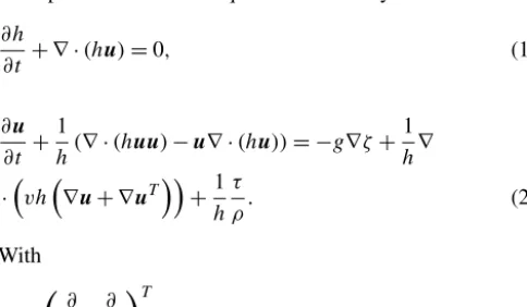
DFM allows the user to schematize the model domain with a flexible mesh in 1-D/2-D/3-D, and therefore supports the computationally efficient schematization of topographically challenging areas such as river bends or irregular slopes. The model solves the full Saint-Venant equations, or SWEs. The main partial differential equations solved by DFM are
∂h
∂t + ∇ ·(hu)=0, (1) ∂u
∂t + 1
h(∇ ·(huu)−u∇ ·(hu))= −g∇ζ+ 1 h∇
·vh∇u+ ∇uT+1
h τ
ρ. (2)
With
∇ =
∂ ∂x,
∂ ∂y
T
, (3)
ζ being the water level, h the water depth, u is the ve-locity vector, g the gravitational acceleration, v the vis-cosity, ρ the water mass density, and τ the bottom fric-tion. For 1-D flow, the equations remain the same ex-cept that the viscosity v does not contain horizontal eddy viscosity. For further technical details and deriva-tion, we refer to the technical manual (Deltares, 2017a). DFM is an openly accessible model and can be obtained by contacting Deltares (https://www.deltares.nl/en/software/
delft3d-flexible-mesh-suite/). Besides riverine flood hazard modelling, it also caters for a wider range of applications, for instance groundwater flow, sediment transport, and water quality simulations in 1-D, 2-D, and 3-D. For more informa-tion regarding the applicainforma-tion of DFM, we refer to the user manual (Deltares, 2017b). Due to its very recent publication, only a limited number of published studies using DFM are available. It was, for instance, applied in a global-scale re-analysis for extreme sea levels (Muis et al., 2016). In another study, Castro Gama et al. (2013) applied DFM to model flood hazard at the Yellow River, and concluded that applying a flexible mesh reduces computation time by a factor of 10 compared to square grids with equal quality of model out-put.
2.3 LISFLOOD-FP (LFP)
LFP is a widely used, raster-based model to compute flood-plain inundation. Since its first version (Bates and de Roo, 2000), it has regularly been adapted and improved (Bates et al., 2010), for instance by adding a sub-gridding scheme to account for channel flow within cells (Neal et al., 2012a).
It is possible to run LFP with different set-ups: a 2-D only, a 1-D, a 1-D/2-D or a sub-grid model, with the latter being the most accurate for large-scale inundation modelling ap-proaches as it greatly increases floodplain connectivity (Neal et al., 2012a).
When using the sub-grid scheme, LFP solves the subse-quent equation for channel flow that is based on a simplifica-tion of the SWE ignoring advecsimplifica-tion (Bates et al., 2010; Neal et al., 2012a). Hereqdenotes the flow per unit width,gthe gravitational acceleration,ζ the water level,Rthe hydraulic radius,nManning’s surface roughness, and∇ the gradients inx- andy-directions as described in Eq. (3):
∂q
∂t + ∇ghζ+ gn2q2
R4/3h=0. (4)
Mass conservation is implemented as
∇(h+q)=0, (5)
whereby1t denotes the time step,1x the cell size andi, j the cell indices. For further information about model devel-opment, derivation of numerical solutions, assumptions, and validations, we refer you to the above-mentioned papers.
LFP is specifically developed to model floodplain inunda-tion and has been used in a wide range of studies. Most no-table in the context of large-scale flood hazard modelling is the work by Sampson et al. (2015), who applied LFP to com-pute global estimates of flood hazard and risk and by Schu-mann et al. (2013) and Biancamaria et al. (2009), who used LFP to simulate inundation in the Zambezi and Ob rivers, respectively, forced with lateral input from a land surface model.
pro-vides all relevant features, in particular the sub-gridding scheme, to model large-scale inundation.
2.4 Basic model interface (BMI)
Generally, the BMI has several functions that can be called from external applications like, as in this case, a Python script. To make these functions available for a model, a BMI adapter needs to be developed for each model with respect to the specific internal model structure and programming lan-guage. Whilst PCR is already written in Python and its BMI implementation is hence straightforward, DFM offers a na-tive C-compliant BMI implementation. For LFP, which is written in C++, the code and file structure had to be slightly adapted to agree with the requirements for the BMI. Once a BMI adapter is developed, it is possible to execute a set of functions: first, the user can initialize the models by us-ing the BMI adapter. Second, the BMI adapter allows for retrieving a set of variables from memory. The variables ex-posed through the BMI adapter can be defined during the development of the BMI adapter and is thus not limited to a preset range. Third, the manipulated variables can be set back to the original model or can be used to overwrite vari-ables in one or multiple other models, given that they agree to the internal data structure of those models. Fourth, mod-els connected to a BMI adapter can be updated at a user-specified time step, hence enabling online coupling of mod-els. In this way it is possible to get, change, and set vari-ables during the execution of the models in use on a time step basis. Last, models can be finalized to end the computa-tions. It is noteworthy that implementing the BMI functions does not alter any functionality or routines in the models. Both DFM and LFP, although not being coded in Python, can be called from within Python using the BMI-python pack-age (see https://github.com/openearth/bmi-python). For fur-ther information regarding the BMI, we refer to Peckham et al. (2013) and the related website (CSDMS, 2016).
3 The computational framework GLOFRIM
The computational framework presented here consists of two key elements, (a) the actual code and (b) a settings-file. Here, a brief overview is given of their main properties. More de-tailed information and an outline is provided in the files themselves.
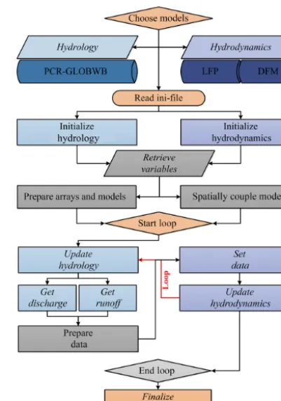
The computational backbone of GLOFRIM is entirely written in Python 2.7 and was developed and tested on Ubuntu systems. By means of a python file (“couplingFrame-work_v1.py” in the downloadable data), the steps for model coupling are executed (see Fig. 1 for a flow chart). The mod-els are first initialized: the model configuration files of each model are read and the internal steps required to obtain an initial state of the models are prompted by the BMI adapter. Thereafter, the BMI adapter is used to retrieve all required
Figure 1.Flow diagram of steps executed in GLOFRIM as well as the model currently available within the framework; all steps in italic are executed by employing the Basic Model Interface (BMI).
thus focus on extending this to a full two-directional cou-pling scheme with feedback loops from hydrodynamics to hydrology. Such two-way coupling would, for instance, con-tain explicit modelling of hydrological processes over inun-dated areas in the hydrodynamic model.
To specify all relevant information about the coupling run to be performed, a configuration file is needed (“default.ini” in the downloadable data). Besides all critical paths to model data, other model settings can be defined in the configuration file, for example the number of model time steps. In general, settings defined in the INI file overrule those specified for the individual models. In the current version of GLOFRIM, three options need to be specified to realize model coupling: by ac-tivating the so-called “River-Floodplain-Scheme” (RFS), by specifying the variables to be updated, and by choosing for hydrodynamic models in either spherical or projected coor-dinate systems.
First, the RFS defines where output from PCR is coupled to. If RFS is activated, water volume of one PCR cell is directly coupled to the 1-D channels of the hydrodynamic model within the corresponding PCR cell. If RFS is inactive, water is distributed over all 2-D grid cells within the corre-sponding PCR cell. Applying the RFS has two major advan-tages: first, it reduces run times as data exchange and com-putations need to be performed for a smaller number of cells; second, using RFS in large-scale applications with sufficient channel information reduces the dependency on the accu-racy of remotely sensed 2-D elevation data such as Shuttle Rader Topographic Mission (SRTM) data (Farr et al., 2007). Recent research showed that such global data sets contain strong vertical bias as well as systematic and random noise (Yamazaki et al., 2017). In particular, simulating flow over vertically irregular terrain resulting in supercritical regimes is contraindicated for LFP because of its use of the LIE. In case overland flow needs to be modelled by LFP, we advise to take measures accordingly, for instance by limiting flow velocities. For DFM we found that runs are more stable, yet slower, when deactivating the RFS.
Second, it is possible to force the hydrodynamic mod-els by updating the water depth variable (in metres) or by updating fluxes, which are expressed in LFP as discharge (in m3s−1) and in DFM as precipitation (in mm d−1). For DFM, added daily water depth is divided into a number of user-specified time steps hence reducing the computational load, while fluxes are daily constants. We found that updat-ing fluxes reduces run times compared to states, and hence advise opting for this option. While it is also possible to per-form state-updating in LFP, test runs showed that this op-tion should be used carefully as it easily increases run times. This is because it is currently not possible to update LFP at a user-specified time step due to the Courant–Friedrichs–Lewy condition. It may hence happen that gradients between added daily water depths are too steep, increasing the risk of model instability. We therefore recommend applying flux-updating in LFP instead.
Third, it is possible to use the hydrodynamic models with Cartesian coordinates, although PCR runs in non-Cartesian coordinates. By providing the projected coordinate system the model is based on, the computational framework can translate the grid into spherical coordinates and perform the grid overlay and cell assignment, thus guaranteeing the ap-plicability of all already existing hydrodynamic schematiza-tions. All other computations remain unaffected by the coor-dinate system in use as the coorcoor-dinate information is solely required for spatially coupling the grids.
As expressed before, GLOFRIM employs the BMI’s func-tionalities to couple hydrological to hydrodynamic pro-cesses. Even though the current version of GLOFRIM only supports one-directional coupling, basing it upon the BMI yields strong advantages for future two-directional coupling as coupled models do not get unnecessarily entangled, so-called “integronsters” (Voinov and Shugart, 2013). Such two-directional coupling is currently not yet available for GLOFRIM due to on-going testing as well as concept de-velopment and will be provided in a future version of the framework.
Besides being openly accessible and thus adaptable and extendable to the user’s preferences or individual modelling requirements, GLOFRIM contains a number of additional advantages: first, by having PCR-GLOBWB, or any other global hydrological model, as the hydrological output cre-ator, the framework can easily be applied anywhere on the globe given a hydrodynamic schematization; second, models to be coupled may be selected depending on their local per-formance, thus possibly capturing more relevant processes; third, the spatially explicit coupling scheme can be extended to a full feedback loop between hydrology and hydrodynamic steps, also incorporating important groundwater infiltration and evaporation processes; fourth, by guaranteeing identical hydrological forcing, applying the computational framework facilitates benchmarking of hydrodynamic models by elimi-nating sources of difference, potentially supporting hydrody-namic ensemble modelling approaches.
4 The synthetic test cases 4.1 Set-up
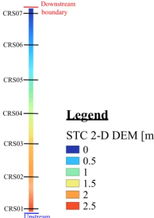
Figure 2.Digital elevation model (DEM) of the 2-D synthetic test case (STC 2-D) for LFP and DFM.
synthetic test cases were forced with an artificial upstream discharge boundary spanning 1 year and consisting of 2 peak flow moments to introduce variability in model dynamics, thus not employing GLOFRIM for those test cases. As down-stream boundary condition, a constant water level of 0 m was set. The entire simulation period was 3 years to ensure it exceeds the time of concentration. To assess model output, 7 cross sections were defined, hence capturing the down-stream propagation of the artificial flood waves and facilitat-ing the assessment of possible attenuation and dampenfacilitat-ing ef-fects. For benchmarking the models, we then compared dis-charge along the cross sections and run times to obtain a first indication of how the different computational schemes might vary (Fig. 2).
4.2 Results and discussion
Assessing the results for both 2-D and 1-D, we find that both models simulate the same responses to the input sig-nal applied (Fig. 3). Due to the higher friction coefficient and the wider flow area, it takes the 2-D schematization al-most the entire simulation period to entirely convey the water volumes to the downstream boundary. In the 1-D schema-tization, however, all water is already drained after around 30 % of the entire simulation period. The similarity of simu-lated discharge between LFP and DFM is, despite the mod-els’ differences in complexity and design, in line with the findings made by Neal et al. (2012b) and De Almeida and Bates (2013). In the latter study, differences in governing equations were assessed analytically for various flow regimes ranging from sub- to supercritical flow. It was concluded that for applications with low Froude numbers (Fr0.5), such
Table 1.Run times of different set-ups in the synthetic test case.
2-D 1-D
DFM 19.5 min 5.5 min LFP 2.1 min 2.6 min
as the synthetic test case used here, no significant differences occur between models solving the LIEs and those solving the full dynamics of the SWEs. Also, Neal et al. (2012b) showed that it seems unnecessary to employ models solv-ing the SWEs for flow gradually varysolv-ing in time and for subcritical flow regimes. In addition, the study showed that for those applications, run times of local inertia models are shorter than those of models solving the full SWEs. The run times measured for the various synthetic test cases used here underpin this finding as LFP exhibits shorter run times, es-pecially for the 2-D schematization (Table 1). To facilitate comparability, we a priori set the maximum solver time step in DFM to the average of the time steps required by LFP. It is noteworthy that the differences in run times may not merely be attributable to varying solver complexity but partially also to the programming language and compiler used as well as to general model complexity and level of code optimization applied.
5 Test case: the Amazon River basin 5.1 Set-up
Figure 3.Simulated discharge of(a)2-D and(b)1-D synthetic test case.
et al. (2011) to derive bathymetry information. For further information, we refer to the relevant papers.
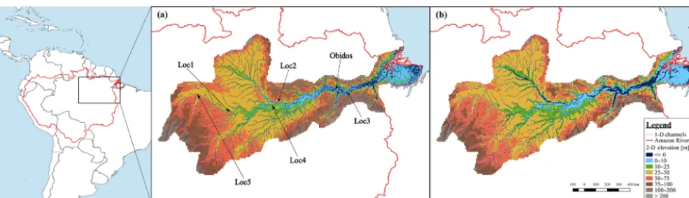
To obtain a LFP schematization equivalent to the DFM schematization, elevation data as well as both river width and river depth information were processed to agree with the requirements of LFP. For river channel properties, the depth and width information stored in the vector data used for DFM were rasterized, and for the elevation data the smoothed canopy-free elevation data were upscaled to a 2 km spatial resolution, employing the nearest neighbour technique, to match the finest spatial resolution of the DFM schematization (Fig. 4). From Fig. 4 it is visible that LFP contains a greater level of detail in areas farther upstream due to the finer spatial resolution uniformly applied. Consequently, the total number of cells in LFP exceeds the number of 2-D cells in DFM by a factor of 4 (Table 2). Furthermore, only around 10 % of the entire schematization represents 1-D channels in LFP, while the channel network of DFM was based on around 30 % of all DFM cells. For both DFM and LFP, Manning’s surface roughness coefficient was uniformly set to 0.03 s m−1/3for channel and floodplains, which is consistent with other case studies in the Amazon (Paiva et al., 2013; Rudorff et al., 2014a, b; Trigg et al., 2009; Yamazaki et al., 2011). As down-stream boundary, we imposed a constant water level of 0 m at the river’s delta. It is noteworthy that GLOFRIM supports the coupling of any hydrodynamic schematization, not only those bordering at a delta but also midstream applications, for instance, if the internal hydrodynamic model requirements are satisfied. Additionally, it should be mentioned that the 1-D channels of both schematizations, even with the GW1-D-LR accounting for islands and thus providing an effective width, do not capture the impact of both braiding and river bifurca-tion, which may potentially impact model results, especially at the river mouth. This is, however, not due to the inability of the hydrodynamic models to account for them, but merely
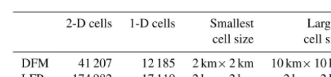
Table 2.Overview of key properties of hydrodynamic schematiza-tions coupled to PCR-GLOBWB in this study.
2-D cells 1-D cells Smallest Largest cell size cell size
DFM 41 207 12 185 2 km×2 km 10 km×10 km LFP 174 982 17 119 2 km×2 km 2 km×2 km
because the chosen algorithm to derive 1-D network proper-ties does not allow for it.
For the hydrological model PCR-GLOBWB, the kine-matic wave approach was used for routing outside of the cou-pled domain. This is required as the hydrodynamic schema-tizations in this test case do not cover the entire extent of the Amazon River basin, even with the kinematic wave ap-proximation potentially introducing an error to the upstream boundary inflow applied. Since simulated discharge from PCR for the Amazon substantially under-predicts observa-tions, we decided to apply an optional regionalized opti-mization technique facilitating comparison between simu-lated and measured discharge values (Hoch et al., 2017a). As such an optimization technique is optional and only ad-visable for catchment studies, a global application is thereby not constrained. In analogy to the hydrodynamic models, the surface roughness coefficient of PCR was uniformly set to 0.03 s m−1/3.
Figure 4.Digital elevation model and 1-D channel network as used in LFP(a)and DFM(b); discharge was benchmarked and validated at Óbidos while water levels were compared at three locations throughout the domain.
The model time covers the period from January 1984 until December 1990 with the first year being used for spin-up of the coupled settings. This period had to be chosen due to the limitation of available GRDC data for model validation. As with the synthetic test case, run times were compared. To be able to understand water-level dynamics as simulated by both models, we compared them at three locations through-out the basin (Fig. 4). The locations were chosen such that they represent the downstream (Loc3), midstream (Loc4), and upstream dynamics in the basin (Loc5). Besides, inun-dation extent was benchmarked by applying three evaluation functions, using the LFP inundation results as the benchmark data set. First, the hit rate H was computed based on the sub-sequent equation:
H=NDFM∩NLFP
NLFP
. (6)
NLFP andNDFM indicate thereby the number of inundated cells in LFP and DFM at the same moment in time, respec-tively. To perform consistent benchmarking, the flexible cells of DFM were resampled to the resolution of LFP. The hit rate can vary between 0, signalling that DFM and LFP have no inundated cells in common and 1, indicating that all cells in LFP are also inundated by DFM.
In addition, we determined the false alarm ratio F to also consider false positive alarms. The false alarm ratio can be obtained with
F= NDFM\NLFP
NDFM∩NLFP+NDFM\NLFP
. (7)
In the optimal situation, F would be 0 showing that no cells are incorrectly marked as flooded in DFM, whereas a value of 1 indicates that all cells are classified as false alarms.
Last, we assessed the critical success index C, which com-bines both hit rate and false alarm ratios into one parame-ter which can vary between 0 in the worst and 1 in the best scenario, indicating perfect match between both inundation
Table 3.Results of Pearson’s coefficientr, root mean square er-ror (RMSE), and Kling–Gupta efficiency (KGE) obtained to bench-mark discharge and run times of coupled runs.
r RMSE KGE Run time
DFM 0.92 25 289 m3 0.76 7 h LFP 0.89 22 291 m3 0.82 6 h
maps:
C=NDFM∩NLFP
NDFM∪NLFP
. (8)
For both set-ups, the River-Floodplain-Scheme was activated and flux-updating was opted for. All simulations were per-formed in a Linux environment with an Intel i7-4790 core at 3.90 GHz and 16 GB memory.
5.2 Results and discussion
Benchmarking discharge results against observation from GRDC at Óbidos shows that both models behave similarly. However, LFP tends to compute earlier peak flow and ear-lier and lower low flow (Fig. 5). Therefore, obtained coef-ficients of correlation are lower for LFP, while the model’s skill as expressed by KGE is higher for LFP and the RMSEs are comparable (Table 3). The general deviation of simulated results to observations can be due to a range of factors, for ex-ample the lack of channel bifurcations in the schematization, the already less-accurate upstream inflow as simulated with the kinematic wave approximation or the general overpredic-tion of discharge by PCR-GLOBWB (Hoch et al., 2017a), but have not been further explored as this would exceed the scope of this study.
Figure 5.Observed discharge (OBS)from the Global Discharge Data Centre (GRDC) as well as simulated discharge from both DFM and LFP at Óbidos.
obtained in the synthetic test case and since the hydrological forcing of both models is equal in terms of water volumes, spatial distribution, and timing, we decided to evaluate the impact of the following parameters: the actual river length and dimension in LFP compared to DFM and the sensitivity of LFP to Manning’s surface roughness coefficient over large areas.
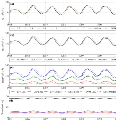
Since the routing scheme of LFP is based on a D4 sys-tem where water can flow in a southerly, northerly, east-erly or westeast-erly direction, channel length and dimension in LFP tend to differ from other hydrodynamic models that are not based on such a system, for example DFM. Reducing or increasing the unitless meandering coefficient in LFP to river-scale dimensions, however, did not show any signifi-cant impact on simulated discharge (Fig. 6a). After investi-gating how changes in surface roughness values in LFP may close the gap to DFM, we indeed found a more pronounced response, yet it cannot satisfactorily explain the difference in simulated discharge either (Fig. 6b). Since in the synthetic example both models can produce near-identical results if us-ing the same friction coefficient and, because the flow regime in the Amazon basin can be described as sub-critical, differ-ent sensitivities to surface roughness over large areas can thus also be disregarded as the cause for discharge discrepancies. For the remaining gap in simulated discharge, we can at this point only make assumptions about the cause. Possible rea-sons include differences in internal processing of 1-D chan-nel bathymetry, chanchan-nel–floodplain interaction, and input el-evation assignment due to the different grid schematizations of a flexible mesh and regular grid.
For a further first-order assessment of a possible impact of spatial resolution, we compared simulated discharge at two stations further upstream, Loc1 and Loc2 (Fig. 4). Results indeed suggest that the differences in upstream spatial reso-lution result in different flood wave propagations (Fig. 6c);
Table 4.Local properties of water level observation stations; input elevation refers to values obtained after hydraulic conditioning of canopy-free SRTM elevation data at 15 arcsec spatial resolution.
Loc3 Loc4 Loc5
Input elevation (m) 4.0 7.0 44.5
Model elevation LFP (m) −0.2 2.4 37.4
Model elevation DFM (m) 0.5 4.9 42.5
Cell area LFP (m2) ∼4×10⁶
Cell area DFM (m2) 7.7×10⁶ 7.7×10⁶ 30.9×10⁶
Figure 6.Results of the sensitivity analysis of(a)the meandering coefficient and(b)both 1-D and 2-D surface roughness coefficients in LFP. Since the D4 system in LFP can both decrease and increase effective river dimension, the dimensionless meandering coefficient was not only reduced from default (1.0) to 0.09, 0.08, and 0.07, but also increased to 1.1, 1.2, and 1.3. As default Manning’s surface roughness is already low (0.03 s m−1/3), coefficients were increased to 0.05, 0.07, and 0.09;(c)Comparison of simulated discharge across basin to assess impact of spatial resolution on simulated discharge; to that end two additional observations upstream of Óbidos were introduced, Loc1 (most upstream) and Loc2 (intermediate upstream);(d)Comparison of simulated water depth at three different locations (Loc3, Loc4, and Loc5) randomly picked within the domain.
their dynamics could not be fully attributed to one specific cause. For example, the more pronounced difference in water levels at Loc1 may be a local effect due to spatial feedback dynamics between neighbouring cells of an observation sta-tion (Hardy et al., 1999), may be related to slight differences in model schematization at the downstream boundary or to backwater effects in the delta regions as a result of different influences of the downstream water level boundary. Further-more, discrepancies are likely to be related to differences in surface elevation simulated at the observation stations due to
the differences in gridding between DFM and LFP. Indeed, assessing the local properties of the observation stations re-vealed that the surface elevation in DFM is higher than in LFP (Table 4). Last, results indicate that differences in grid-ding and therefore cell size may thus have locally impacted the overall water levels too since the above-discussed dis-charge simulations in upstream areas exhibited clear devia-tions between both models (Fig. 6c).
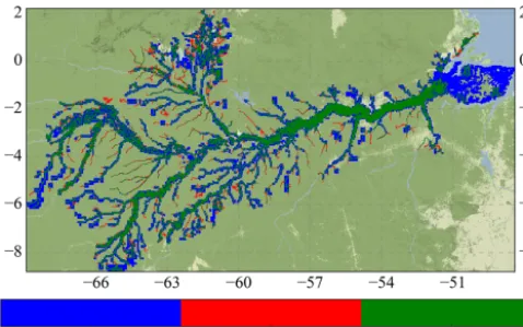
simula-Figure 7.Benchmarking simulated inundation extent by DFM and LFP.
tion period of 7 years, that is model time plus spin-up, while performing the same simulation with DFM takes around 7 h (Table 3). The difference in run times is less pronounced than for the synthetic test case, which can be related to the lower number of cells in DFM compared to LFP due to use of a flexible mesh. In addition, a more computationally expensive interaction between the 1-D and 2-D domain in DFM could also affect run times. As DFM is in general a multi-purpose tool whose application is not limited to inundation mod-elling, it is not unexpected that it may be slightly slower than programmes specifically tailored for efficient large-scale in-undation modelling such as LFP.
We find that inundation extents obtained at the end of the simulation runs with DFM and LFP are comparable, yet far from identical (Fig. 7). Due to the larger inundation extent of DFM, a hit rate of 0.85 is obtained, indicating that 85 % of extent as simulated by LFP is also simulated by DFM. Espe-cially differences in inundated extent in upstream areas and along small reaches can explain the obtained false alarm ratio of 0.50 (Table 5). These differences are also responsible for the critical success index of 0.46 corroborating that in bit less than half of the cells inundation extent is simulated by both models. A model agreement of 46 % is slightly higher than the 30–40 % found by Trigg et al. (2016) for a benchmarking study of global flood hazard models. This, in fact, suggests that the choice of numerical scheme and model schematiza-tion alone can greatly impact upon inundaschematiza-tion, confirming that differences in model forcing and boundary conditions do not act alone as a cause of modelled inundation differ-ence, which could have been the case in the results obtained by Trigg et al. (2016).
A main cause for the differences observed for regions fur-ther upstream is that DFM tends to compute larger flood ex-tent than LFP: with DFM having larger cells in upstream areas due to the flexible meshing, a larger 2-D area is in-stantly marked as inundated for DFM once overbank flow occurs. This loss of level of detail in DFM is the concession to be made for a reduced number of grid cells and hence
po-Table 5.Resulting hit rate H, false alarm ratio F, and critical success index C for benchmarking inundation extent.
H F C
LFP/DFM 0.85 0.50 0.46
tentially faster computations in the 2-D domain. For more downstream regions, differences in inundation extent are pri-marily present at small river channels while floodplain in-undation is comparable. This, however, can to some extent be attributed to differences in how the 1-D domain is imple-mented in the models, with DFM using grid-size independent vectors and LFP using grids at the overall spatial resolution of the schematization. Given the overall larger inundation ex-tent simulated by DFM, the above-discussed deviations in simulated discharge and in particular the more pronounced wave attenuation in DFM may be explained as return flows from the floodplain to the channel as they seem to be faster in LFP than in DFM.
6 Conclusion and recommendations
In this study, we presented GLOFRIM, a GLObally applica-ble computational FRamework for Integrated hydrological– hydrodynamic Modelling. In its current version, it provides an environment to one-directionally couple the global hy-drological model PCR-GLOBWB with two hydrodynamic models: Delft3D Flexible Mesh solving the full SWEs, and LISFLOOD-FP solving the LIEs. By linking hydrol-ogy to hydrodynamics, it is possible to take advantage of the strengths of both while at the same time compensating their weaknesses.
We define five main assets of GLOFRIM: (i) it is openly accessible and hence can be directly applied and adapted to specific purposes, and extended with other models; (ii) by employing a global hydrological model to obtain model forc-ing, the framework can easily be applied globally; (iii) mod-els to be coupled may be selected depending on their local performance and thus more relevant processes can be cap-tured; (iv) the spatially explicit coupling scheme can be ex-tended to a full feedback loop between hydrology and hydro-dynamics; (v) thorough benchmarking and ensemble mod-elling of hydrodynamic models is supported by providing identical hydrological forcing for experiments.
Besides PCR as well as DFM and LFP, there are many other global hydrological and hydrodynamic models avail-able which have their individual advantages. As the frame-work is freely and openly available, its design can easily be extended and adapted to cater for the coupling of other hydrological or hydrodynamic models, merely requiring the implementation of the BMI into each model to be added. Eventually, adding a 1-D continental hydrodynamic model such as CaMa-Flood (Yamazaki et al., 2011) would allow for replacing the kinematic wave approximation of PCR to provide more accurate upstream boundary inflow to the do-main with explicit high-resolution 2-D floodplain computa-tions. Employing a BMI does not change the model function-ality but it does provide a range of added functions. Further-more, not all model variables need to be exposed, only those to reproduce model geometry, distinguish between 1-D and 2-D cells, and to update model states. We therefore recom-mend considering this option for future model developments and will also aim to incorporate other models ourselves. To our knowledge, spatially explicit model coupling on a global scale by means of such a framework is unprecedented. Con-sequently, user experiences and lessons learnt are still sparse and any initiatives regarding framework extension are there-fore kindly received by the authors, as well as feedback and experiences. We also recommend the testing and application of it in other study areas and under different boundary con-ditions to further evaluate the code, process flow, and appli-cability.
Before applying GLOFRIM in an actual test case, we per-formed a simple synthetic test case to obtain a first-order in-sight into how both models may differ regarding their com-putational complexity. Thereby both the 1-D and 2-D domain were forced by a synthetic inflow signal and simulated dis-charge was evaluated along the flow path. Results show that both models produce the same response to the signal despite the difference in solver complexity. The results obtained are in line with previous studies showing that for sub-critical flow regimes discharge results should be similar (De Almeida and Bates, 2013; Neal et al., 2012b).
Both hydrodynamic models were then applied within GLOFRIM for the Amazon River basin and evaluated re-garding simulated discharge, water levels, run time, and in-undation extent, also constituting a first comparison of large-scale flexible mesh and regular grid applications. Assessing simulated discharge shows that both models exhibit com-parable results with LFP tending to compute earlier and slightly increased peak discharge estimates. As thorough testing of plausible causes did not show significant improve-ments, we speculate that differences in processing of 1-D channel bathymetry, interaction between 1-D channels and 2-D floodplains or assignment of input surface elevation data to the different grids may impact discharge results. The latter is supported by discharge observations made in farther up-stream areas where differences in grids are largest. A more in-depth analysis of these differences was, however, outside
the scope of this study and thus needs to be performed in a follow-up study. As the general overprediction of observed discharge at Óbidos can partly be attributed to the absence of hydrological processes on inundated floodplains, it is envis-aged to extend the current code such that it also caters for a full feedback loop between hydrodynamics and hydrology.
Water levels simulated by both models differ locally, yet only slightly. These discrepancies between both models are most likely due different grid schematizations in DFM and LFP, which results in locally differing elevation values and cell areas and thus influences simulated water levels. Due to differences in model structure and design, downstream boundary conditions had to be implemented slightly differ-ently, possibly also impacting water level results in particu-lar for more downstream stations. As it was the aim of this paper to introduce the computational framework applied, a more elaborated evaluation of causes for water level devia-tions is future work.
A key parameter for large-scale modelling is run time. In the current study, the schematization of LFP contains more than 4 times the number of 2-D cells than DFM while the number of 1-D cells is 40 % higher in LFP than in DFM. De-spite the greater number of cells, LFP has a slightly shorter run time. This is in line with the results obtained in the syn-thetic test case, yet the relative difference is reduced due to the application of flexible meshes for the 2-D domain and the nature of the coupling algorithm applied: because water was coupled directly into the 1-D channels, flow over the 2-D domain was limited and, as a result, so was the impact of differences in computational efficiency of the models. Dif-ferences in run times may also be related to more fundamen-tal factors, such as the degree of code optimization applied. Additionally, DFM was, in contrast to LFP, not explicitly de-veloped for efficient inundation modelling, but as a multi-purpose tool including several additional physical processes, such as the potential to simulate 3-D flow, estuarine pro-cesses or hydrogeomorphologic dynamics, which could also result in longer run times. To better understand causes of run time discrepancies, further model development, testing, and evaluation is therefore recommended.
run times, they may also have implications for detailed flood hazard estimates which can be strongly hampered. In the case of employing a flexible mesh, it seems as if an a priori deci-sion has to be made where and to which extent such models are supposed to provide fine-scale results or whether compu-tational efficiency is the main aim – both at the same time does not seem to be feasible from our results. We hence rec-ommend testing the application of flexible meshes for large-scale riverine inundation modelling in more detail to obtain a better understanding of the trade-off to be made between grid refinement and model accuracy.
With the presented computational framework GLOFRIM and the satisfactory results obtained, we trust to have con-tributed to the current development of model coupling and integration, and to have provided an openly accessible tool that facilitates more accurate large-scale flood hazard esti-mates. We hope that, eventually, the integration of hydrolog-ical and hydrodynamic models will lead to improved flood risk assessments and planning of climate change impact mit-igation and adaption measures.
Code and data availability. The code of GLOFRIM and the BMI versions of LISFLOOD-FP and PCR-GLOBWB are openly accessible and freely downloadable at https://doi.org/10.5281/zenodo.597107 (Hoch et al., 2017b).
Author contributions. FB and JMH developed the BMI adapter for LISFLOOD-FP. JMH, RvB, and JCN developed the code of the computational framework. JCN, RvB, HCW, PDB, and MFPB su-pervised the research and provided important advice. JMH designed and executed the research, and also prepared the manuscript as well as code, with contribution from all co-authors.
Competing interests. The authors declare that they have no conflict of interest. Author Jeffrey C. Neal is a topical editor of the journal.
Acknowledgements. This study was financed by the EIT Climate-KIC programme under project title “Global high-resolution database of current and future river flood hazard to support plan-ning, adaption and re-insurance”. We also want to acknowledge the contributions of Climate-KIC and University of Bristol to realize a research stay at the University of Bristol. Special thanks are reserved for Arthur van Dam and Herman Kernkamp from Deltares for their support in applying Delft3D Flexible Mesh and Edwin Sutanudjaja for PCR-GLOBWB advice. Last, we want to express our gratitude to an anonymous reviewer and Dai Yamazaki for evaluating a previous version of the manuscript and providing invaluable feedback.
Edited by: Bethanna Jackson
Reviewed by: Dai Yamazaki and one anonymous referee
References
Alcamo, J., Döll, P., Kasper, F., and Siebert, S.: Global change and global scenarios of water use and availability: An Application of WaterGAP1.0., 1997.
Bates, P. D. and de Roo, A.: A simple raster-based model for flood inundation simulation, J. Hydrol., 236, 54–77, https://doi.org/10.1016/S0022-1694(00)00278-X, 2000. Bates, P. D., Horritt, M. S., and Fewtrell, T. J.: A simple inertial
formulation of the shallow water equations for efficient two-dimensional flood inundation modelling, J. Hydrol., 387, 33–45, https://doi.org/10.1016/j.jhydrol.2010.03.027, 2010.
Baugh, C. A., Bates, P. D., Schumann, G. J.-P., and Trigg, M. A.: SRTM vegetation removal and hydrodynamic modeling accuracy, Water Resour. Res., 49, 5276–5289, https://doi.org/10.1002/wrcr.20412, 2013.
Beven, K. J., Cloke, H. L., Pappenberger, F., Lamb, R., and Hunter, N. M.: Hyperresolution information and hyperresolution igno-rance in modelling the hydrology of the land surface, Sci. China Earth Sci., 58, 25–35, https://doi.org/10.1007/s11430-014-5003-4, 2015.
Biancamaria, S., Bates, P. D., Boone, A., and Mognard, N. M.: Large-scale coupled hydrologic and hydraulic modelling of the Ob river in Siberia, J. Hydrol., 379, 136–150, https://doi.org/10.1016/j.jhydrol.2009.09.054, 2009.
Bierkens, M. F. P.: Global hydrology 2015: State, trends, and directions, Water Resour. Res., 51, 4923–4947, https://doi.org/10.1002/2015WR017173, 2015.
Castro Gama, M., Popescu, I., Mynett, A., Shengyang, L., and van Dam, A.: Modelling extreme flood hazard events on the middle Yellow River using DFLOW-flexible mesh approach, Nat. Haz-ards Earth Syst. Sci. Discuss., https://doi.org/10.5194/nhessd-1-6061-2013, 2013.
Ceola, S., Laio, F., and Montanari, A.: Satellite night-time lights reveal increasing human exposure to floods worldwide, Geophys. Res. Lett., 41, 7184–7190, https://doi.org/10.1002/2014GL061859, 2014.
Clarke, R. T., Mendiondo, E. M., and Brusa, L. C.: Uncertain-ties in mean discharges from two large South American rivers due to rating curve variability, Hydrol. Sci. J., 45, 221–236, https://doi.org/10.1080/02626660009492321, 2000.
CSDMS: CSDMS Basic Model Interface (version 1.0), available at: https://csdms.colorado.edu/wiki/BMI_Description, last access: 25 August 2016.
CSDMS: CSDMS Web Modeling Tool, available at: https://csdms. colorado.edu/wmt/, last access: 2 February 2017.
Dadson, S. J., Ashpole, I., Harris, P., Davies, H. N., Clark, D. B., Blyth, E., and Taylor, C. M.: Wetland inundation dynam-ics in a model of land surface climate: Evaluation in the Niger inland delta region, J. Geophys. Res.-Atmos., 115, 1–7, https://doi.org/10.1029/2010JD014474, 2010.
De Almeida, G. A. M. and Bates, P. D.: Applicability of the local inertial approximation of the shallow water equa-tions to flood modeling, Water Resour. Res., 49, 4833–4844, https://doi.org/10.1002/wrcr.20366, 2013.
Deltares: Delft3D Flexible Mesh Technical Manual, avail-able at: https://content.oss.deltares.nl/delft3d/manuals/D-Flow_ FM_Technical_Reference_Manual.pdf, last access: 3 Febru-ary 2017a.
Deltares: Delft3D Flexible Mesh User Manual, available at: https://content.oss.deltares.nl/delft3d/manuals/D-Flow_FM_ User_Manual.pdf, last access: 3 February 2017b.
Döll, P., Kaspar, F., and Lehner, B.: A global hydrological model for deriving water availability indicators: model tuning and vali-dation, J. Hydrol., 270, 105–134, https://doi.org/10.1016/S0022-1694(02)00283-4, 2003.
Dottori, F., Salamon, P., Bianchi, A., Alfieri, L., Hirpa, F., and Feyen, L.: Development and evaluation of a framework for global flood hazard mapping, Adv. Water Resour., 94, 87–102, https://doi.org/10.1016/j.advwatres.2016.05.002, 2016. FAO: FAOSTAT, available at: http://www.fao.org/faostat/en/#home,
last access: 13 January 2017.
Farr, T. G., Rosen, P. A., Caro, E., Crippen, R., Duren, R., Hensley, S., Kobrick, M., Paller, M., Rodriguez, E., Roth, L., Seal, D., Shaffer, S., Shimada, J., Umland, J., Werner, M., Oskin, M., Burbank, D., and Alsdorf, D.: The Shut-tle Radar Topography Mission, Rev. Geophys., 45, RG2004, https://doi.org/10.1029/2005RG000183, 2007.
Gupta, H. V., Kling, H., Yilmaz, K. K., and Martinez, G. F.: Decom-position of the mean squared error and NSE performance crite-ria?: Implications for improving hydrological modelling, J. Hy-drol., 377, 80–91, https://doi.org/10.1016/j.jhydrol.2009.08.003, 2009.
Hardy, R. J., Bates, P. D., and Anderson, M. G.: The importance of spatial resolution in hydraulic models for floodplain environ-ments, J. Hydrol., 216, 124–136, https://doi.org/10.1016/S0022-1694(99)00002-5, 1999.
Harris, I., Jones, P. D., Osborn, T. J., and Lister, D. H.: Up-dated high-resolution grids of monthly climatic observations – the CRU TS3.10 Dataset, Int. J. Climatol., 34, 623–642, https://doi.org/10.1002/joc.3711, 2014.
Hirabayashi, Y., Mahendran, R., Koirala, S., Konoshima, L., Ya-mazaki, D., Watanabe, S., Kim, H., and Kanae, S.: Global flood risk under climate change, Nat. Publ. Gr., 3, 816–821, https://doi.org/10.1038/nclimate1911, 2013.
Hoch, J. M., Haag, A. V., van Dam, A., Winsemius, H. C., van Beek, L. P. H., and Bierkens, M. F. P.: Assessing the impact of hydro-dynamics on large-scale flood wave propagation – a case study for the Amazon Basin, Hydrol. Earth Syst. Sci., 21, 117–132, https://doi.org/10.5194/hess-21-117-2017, 2017a.
Hoch, J. M., Baart, F., Neal, J. C., van Beek, R., Winsemius, H. C., Bates, P. D., and Bierkens, M. F. P.: GLOFRIM code repository, available at: https://doi.org/10.5281/zenodo.597107, last access: 24 October 2017b.
Jongman, B., Hochrainer-Stigler, S., Feyen, L., Aerts, J. C. J. H., Mechler, R., Botzen, W. J. W., Bouwer, L. M., Pflug, G., Rojas, R., and Ward, P. J.: Increasing stress on disaster-risk finance due to large floods, Nat. Clim. Chang., 4, 1–5, https://doi.org/10.1038/NCLIMATE2124, 2014.
Kållberg, P., Berrisford, P., Hoskins, B. J., Simmons, A. J., Uppala, S., Lamy-Thepaut, S., and Hine, R.: ERA-40 atlas, ERA-40 Proj. Rep. Ser. 19, Eur. Cent. for Medium Range Weather Forecasts, Reading, UK, 2005.
Karssenberg, D., Schmitz, O., Salamon, P., de Jong, K., and Bierkens, M. F. P.: A software framework for construc-tion of process-based stochastic spatio-temporal models and data assimilation, Environ. Model. Softw., 25, 489–502, https://doi.org/10.1016/j.envsoft.2009.10.004, 2010.
Kernkamp, H. W. J., van Dam, A., Stelling, G. S., and de Goede, E. D.: Efficient scheme for the shallow water equations on un-structured grids with application to the Continental Shelf, Ocean Dyn., 61, 1175–1188, https://doi.org/10.1007/s10236-011-0423-6, 2011.
Kim, J., Warnock, A., Ivanov, V. Y., and Katopodes, N. D.: Coupled modeling of hydrologic and hydrodynamic processes including overland and channel flow, Adv. Water Resour., 37, 104–126, https://doi.org/10.1016/j.advwatres.2011.11.009, 2012. Li, H., Beldring, S., and Xu, C.-Y.: Stability of model
per-formance and parameter values on two catchments facing changes in climatic conditions, Hydrol. Sci. J., 60, 1317–1330, https://doi.org/10.1080/02626667.2014.978333, 2015.
Lian, Y., Chan, I.-C., Singh, J., Demissie, M., Knapp, V., and Xie, H.: Coupling of hydrologic and hydraulic mod-els for the Illinois River Basin, J. Hydrol., 344, 210–222, https://doi.org/10.1016/j.jhydrol.2007.08.004, 2007.
Liang, X., Lettenmaier, D. P., Wood, E. F., and Burges, S. J.: A sim-ple hydrologically based model of land surface water and energy fluxes for general circulation models, J. Geophys. Res.-Atmos., 99, 14415–14428, https://doi.org/10.1029/94JD00483, 1994. Mahe, G., Bamba, F., Soumaguel, A., Orange, D., and Olivry,
J. C.: Water losses in the inner delta of the River Niger: wa-ter balance and flooded area, Hydrol. Process., 23, 3157–3160, https://doi.org/10.1002/hyp.7389, 2009.
Meade, R. H., Rayol, J. M., Conceição, da Conceição, S. C., and Natividade, J. R. G.: Backwater Effects in the Ama-zon River of Basin, Environ. Geol. Water Sci., 18, 105–114, https://doi.org/10.1007/BF01704664, 1991.
Moussa, R. and Bocquillon, C.: Criteria for the choice of flood-routing methods in natural channels, J. Hydrol., 186, 1–30, https://doi.org/10.1016/S0022-1694(96)03045-4, 1996. Muis, S., Verlaan, M., Winsemius, H. C., Aerts, J. C. J. H.,
and Ward, P. J.: Corrigendum: A global reanalysis of storm surges and extreme sea levels, Nat. Commun., 7, 12913, https://doi.org/10.1038/ncomms12913, 2016.
Munich Re: Munich Reinsurance Company Geo Risks Research, NatCatSERVICE Database, 2013.
Neal, J. C., Schumann, G. J.-P., and Bates, P. D.: A subgrid channel model for simulating river hydraulics and floodplain inundation over large and data sparse areas, Water Resour. Res., 48, 1–16, https://doi.org/10.1029/2012WR012514, 2012a.
Neal, J. C., Villanueva, I., Wright, N., Willis, T., Fewtrell, T., and Bates, P. D.: How much physical complexity is needed to model flood inundation?, Hydrol. Process., 26, 2264–2282, https://doi.org/10.1002/hyp.8339, 2012b.
O’Loughlin, F. E., Paiva, R. C. D., Durand, M., Alsdorf, D. E., and Bates, P. D.: A multi-sensor approach towards a global vegetation corrected SRTM DEM product, Remote Sens. Environ., 182, 49– 59, https://doi.org/10.1016/j.rse.2016.04.018, 2016.
Paiva, R. C. D., Collischonn, W., and Buarque, D. C.: Vali-dation of a full hydrodynamic model for large-scale hydro-logic modelling in the Amazon, Hydrol. Process., 27, 333–346, https://doi.org/10.1002/hyp.8425, 2013.
Pappenberger, F., Dutra, E., Wetterhall, F., and Cloke, H. L.: Deriv-ing global flood hazard maps of fluvial floods through a phys-ical model cascade, Hydrol. Earth Syst. Sci., 16, 4143–4156, https://doi.org/10.5194/hess-16-4143-2012, 2012.
Peckham, S. D., Hutton, E. W. H., and Norris, B.: A component-based approach to integrated modeling in the geo-sciences: The design of CSDMS, Comput. Geosci., 53, 3–12, https://doi.org/10.1016/j.cageo.2012.04.002, 2013.
Rennó, C. D., Nobre, A. D., Cuartas, L. A., Soares, J. V., Hod-nett, M. G., Tomasella, J., and Waterloo, M. J.: HAND, a new terrain descriptor using SRTM-DEM: Mapping terra-firme rain-forest environments in Amazonia, Remote Sens. Environ., 112, 3469–3481, https://doi.org/10.1016/j.rse.2008.03.018, 2008. Rudorff, C. M., Melack, J. M., and Bates, P. D.:
Flood-ing dynamics on the lower Amazon floodplain: 1. Hy-draulic controls on water elevation, inundation extent, and river-floodplain discharge, Water Resour. Res., 50, 619–634, https://doi.org/10.1002/2013WR014091, 2014a.
Rudorff, C. M., Melack, J. M., and Bates, P. D.: Flooding dynam-ics on the lower Amazon floodplain: 2. Seasonal and interan-nual hydrological variability, Water Resour. Res., 50, 635–649, https://doi.org/10.1002/2013WR014714, 2014b.
Sampson, C. C., Smith, A. M., Bates, P. D., Neal, J. C., Alfieri, L., and Freer, J. E.: A high-resolution global flood hazard model, Water Resour. Res., 51, 7358–7381, https://doi.org/10.1002/2015WR016954, 2015.
Schumann, G. J.-P., Neal, J. C., Voisin, N., Andreadis, K. M., Pappenberger, F., Phanthuwongpakdee, N., Hall, A. C., and Bates, P. D.: A first large-scale flood inunda-tion forecasting model, Water Resour. Res., 49, 6248–6257, https://doi.org/10.1002/wrcr.20521, 2013.
Tayefi, V., Lane, S. N., Hardy, R. J., and Yu, D.: A comparison of one- and two-dimensional approaches to modelling flood inun-dation over complex upland floodplains, Hydrol. Process., 21, 3190–3202, https://doi.org/10.1002/hyp.6523, 2007.
Trigg, M. A., Wilson, M. D., Bates, P. D., Horritt, M. S., Alsdorf, D. E., Forsberg, B. R., and Vega, M. C.: Amazon flood wave hydraulics, J. Hydrol., 374, 92–105, https://doi.org/10.1016/j.jhydrol.2009.06.004, 2009.
Trigg, M. A., Birch, C. E., Neal, J. C., Bates, P. D., Smith, A., Sampson, C. C., Yamazaki, D., Hirabayashi, Y., Pappenberger, F., Dutra, E., Ward, P. J., Winsemius, H. C., Salamon, P., Dot-tori, F., Rudari, R., Kappes, M. S., Simpson, A. L., Hadzi-lacos, G., and Fewtrell, T. J.: The credibility challenge for global fluvial flood risk analysis, Environ. Res. Lett., 11, 94014, https://doi.org/10.1088/1748-9326/11/9/094014, 2016.
Uppala, S. M., Kållberg, P. W., Simmons, A. J., Andrae, U., Bech-told, V. D. C., Fiorino, M., Gibson, J. K., Haseler, J., Hernandez, A., Kelly, G. A., Li, X., Onogi, K., Saarinen, S., Sokka, N., Al-lan, R. P., Andersson, E., Arpe, K., Balmaseda, M. A., Beljaars, A. C. M., Berg, L. Van De, Bidlot, J., Bormann, N., Caires, S., Chevallier, F., Dethof, A., Dragosavac, M., Fisher, M., Fuentes, M., Hagemann, S., Hólm, E., Hoskins, B. J., Isaksen, L., Janssen, P. A. E. M., Jenne, R., Mcnally, A. P., Mahfouf, J.-F., Morcrette, J.-J., Rayner, N. A., Saunders, R. W., Simon, P., Sterl, A.,
Tren-berth, K. E., Untch, A., Vasiljevic, D., Viterbo, P. and Woollen, J.: The ERA-40 re-analysis, Q. J. Roy. Meteor. Soc., 131, 2961– 3012, https://doi.org/10.1256/qj.04.176, 2005.
van Beek, L. P. H.: Forcing PCR-GLOWB with CRU data, De-partment of Physical Geography, Utrecht University, available at: http://vanbeek.geo.uu.nl/suppinfo/vanbeek2008.pdf (last access: 25 September 2017), 2008.
van Beek, L. P. H. and Bierkens, M. F. P.: The Global Hydro-logical Model PCR-GLOBWB: Conceptualization, Parameter-ization and Verification, available at: http://vanbeek.geo.uu.nl/ suppinfo/vanbeekbierkens2009.pdf (last access: 25 September 2017), 2008.
van Beek, L. P. H., Wada, Y., and Bierkens, M. F. P.: Global monthly water stress: 1. Water balance and water availability, Water Resour. Res., 47, W07517, https://doi.org/10.1029/2010WR009791, 2011.
Visser, H., Bouwman, A., Ligtvoet, W., and Petersen, A. C.: A statistical study of weather-related disasters: past, present and future, PBL Netherlands Environ. Assess. Agency, Hague/Bilthoven, Netherlands, 2012.
Voinov, A. and Shugart, H. H.: “Integronsters”, integral and integrated modeling, Environ. Model. Softw., 39, 149–158, https://doi.org/10.1016/j.envsoft.2012.05.014, 2013.
Wanders, N. and Wada, Y.: Human and climate impacts on the 21st century hydrological drought, J. Hydrol., 526, 208–220, https://doi.org/10.1016/j.jhydrol.2014.10.047, 2015.
Ward, P. J., Jongman, B., Salamon, P., Simpson, A., Bates, P. D., de Groeve, T., Muis, S., de Perez, E. C., Rudari, R., Trigg, M. A., and Winsemius, H. C.: Usefulness and limita-tions of global flood risk models, Nat. Clim. Chang., 5, 712–715, https://doi.org/10.1038/nclimate2742, 2015.
Winsemius, H. C., Van Beek, L. P. H., Jongman, B., Ward, P. J., and Bouwman, A.: A framework for global river flood risk assessments, Hydrol. Earth Syst. Sci., 17, 1871–1892, https://doi.org/10.5194/hess-17-1871-2013, 2013.
Winsemius, H. C., Aerts, J. C. J. H., van Beek, L. P. H., Bierkens, M. F. P., Bouwman, A., Jongman, B., Kwadijk, J. C. J., Ligtvoet, W., Lucas, P. L., van Vuuren, D. P., and Ward, P. J.: Global drivers of future river flood risk, Nat. Clim. Chang., 6, 381–385, https://doi.org/10.1038/nclimate2893, 2016.
Wood, E. F., Lettenmaier, D. P., and Zartarian, V. G.: A land-surface hydrology parameterization with subgrid variability for general circulation models, J. Geophys. Res., 97, 2717, https://doi.org/10.1029/91JD01786, 1992.
World Resources Institute: Aqueduct Global Flood Analyzer, avail-able at: http://floods.wri.org, last access: 17 June 2017.
Yamazaki, D., Kanae, S., Kim, H., and Oki, T.: A physi-cally based description of floodplain inundation dynamics in a global river routing model, Water Resour. Res., 47, 1–21, https://doi.org/10.1029/2010WR009726, 2011.
Yamazaki, D., Baugh, C. A., Bates, P. D., Kanae, S., Alsdorf, D. E., and Oki, T.: Adjustment of a spaceborne DEM for use in floodplain hydrodynamic modeling, J. Hydrol., 436–437, 81–91, https://doi.org/10.1016/j.jhydrol.2012.02.045, 2012.
Yamazaki, D., Ikeshima, D., Tawatari, R., Yamaguchi, T., O’Loughlin, F., Neal, J. C., Sampson, C. C., Kanae, S., and Bates, P. D.: A high-accuracy map of global terrain elevations, Geophys. Res. Lett., 44, 5844–5853, https://doi.org/10.1002/2017GL072874, 2017.