Urban Noise Analysis using Multinomial Logistic Regression
1
Dermot Geraghty, Assistant Professor, Department of Mechanical & Manufacturing 2
Engineering, Trinity College Dublin, Dublin 2, Ireland. Tel: +353 1 8961042 Fax: +353 1 3
6795554 Email: [email protected]
4
Margaret O’Mahony, (Corresponding author), Professor of Civil Engineering, Centre for 5
Transport Research, Department of Civil, Structural & Environmental Engineering, Trinity 6
College Dublin, Dublin 2, Ireland 7
Tel: + 353 1 8962084, Email: [email protected] 8
9
Published as: Geraghty, D. and O'Mahony, M., Urban noise analysis using multinomial
10
logistic regression, Journal of Transportation Engineering, American Society of Civil
11
Engineers, 2016, p04016020-1 – 11. http://dx.doi.org/10.1061/(ASCE)TE.1943-12
5436.0000843#sthash.VLm7XSUO.dpuf
13
14
Abstract
15
The research uses a database of urban noise data collected continually from April 2013 to 16
March 2014 at ten sites in Dublin, Ireland. The first objective of the paper is to investigate if 17
the morning daily noise level peak is related to transport characteristics of households, such 18
as, car ownership levels, the mode by which people travel to work and morning work trip 19
departure time. Data from the 2011 Irish census is used to provide the information on 20
households and this is tested against noise measurement levels. The second objective is to 21
examine the relative importance of the spatial and temporal variables of location, month of 22
the year, weekday and hour of the day, in predicting urban noise levels using a multinomial 23
logistic regression model. The results show that the transport household characteristics 24
demonstrates that location is the most important variable followed in order by hour of the 26
day, month of the year and weekday, in predicting urban noise levels. 27
28
29
Introduction
30
Noise in urban environments can be a major source of concern from health and quality of life 31
perspectives. Economic demands on urban areas create the need for transport and other 32
activities that generate noise. Noise research spans the health sector, the environment and the 33
transport sector. Recent research in the health sector includes work by Halperin (2014) who 34
found that there is emerging evidence that short-term effects of environmental noise, 35
particularly when the exposure is nocturnal, maybe followed by long-term adverse cardio 36
metabolic outcomes. Tobías et al (2015) found that exposure to traffic noise should be 37
considered an important environmental factor having a significant impact on health. Sygna et 38
al (2014) found that road traffic noise may be associated with poorer mental health among 39
subjects with poor sleep. 40
41
Other research focuses on noise measurement and modelling. Mehdi (2011) et al studied the 42
spatial and temporal patterns of noise exposure due to road traffic in Karachi and found the 43
average value of noise levels to be over 66 dB, with maximum peaks over 101 dB, which is 44
close to 110 dB, the level that can cause possible hearing impairment according to the WHO 45
guidelines. Koushki et al (1993) monitored traffic noise at 42 locations in 13 districts in 46
Riyadh, Saudi Arabia and interviewed 2,095 individual heads of household at the noise 47
monitoring sites to determine their perceptions and attitudes toward urban traffic noise. As 48
might be expected, people living and working along major arterials and freeways were 49
51
52
Characterisation of Noise in Urban areas using Transport Related Household
53
Characteristics
54
Camusso (2007) attempted to define alternative noise indicators that would be able to 55
characterise better the acoustic climate in urban environments. He used the idea of defining a 56
set of standard sites that incorporate a combination of simple characteristics of a section of 57
urban street e.g. number of lanes, presence of trams etc. Sites with certain geometric 58
configurations were found to be more linked to the highest noise levels. Weber et al (2014) 59
found that landscape metrics, construction height and total build area reduces noise levels in 60
neighbourhoods. Land use class metrics included e.g. whether the location was city centre 61
based or a low-density single house development in a built up area or had more high-quality 62
detached houses supplemented by private gardens in the area. They found that landscape 63
metrics are relevant and promising indicators for estimation of noise levels in the case of city 64
land-use/structural changes but noted that structural parameters such as building height must 65
also be considered. Silva et al (2014) used urban form as a proxy on the noise exposure of 66
buildings. The work described above demonstrates the demand for characterisation of noise 67
at different sites on the basis of a wide range of different types of variables. 68
With recent research, Lavandier et al, 2015, focusing on the development and 69
characterisation of ‘quiet zones’ in cities, as defined by the European directive 2002/49/EC 70
(EC, 2002), there is a recognition that noise levels are a function of human activity and can 71
be curtailed by local authorities to a certain degree. The difference noted by Geraghty et al 72
(2015) between noise levels in busy urban sites and designated ‘quiet areas’ suggests that 73
that areas with high levels of car ownership and usage levels with high numbers of people 75
departing an area for work in the morning peak period may well show characteristically 76
higher noise levels than areas with lower values of these variables. Little work has been done 77
on the characterisation of site noise levels using variables at the household level e.g. transport 78
characteristics such as car ownership levels, work trip start time etc and this forms the basis 79
of one of the research questions addressed in this paper. 80
Relative Importance of Spatial and Temporal Variables
81
In addition to the research question identified above, a further exploration of the impact of 82
location and temporal variables on noise levels is also investigated in the paper. The 83
following background presents the case for this second research objective. A number of 84
studies have focused on the variables that influence noise levels with attempts to characterise 85
soundscapes on the basis of those variables or to prioritise variables in terms of their 86
contribution to noise levels. Ruiz-Padillo (2014) proposed a methodology to sort, by priority, 87
road stretches requiring appropriate action, identified by their noise problems using a 88
selection of road stretch priority variables weighted according to their influence on the road 89
traffic noise problem. Mateus et al (2015) looked at the influence of the sampling parameters 90
on the uncertainty of the equivalent continuous noise level in environmental noise 91
measurements. They found, for short term measurements, not only the integration time but 92
also the number of samples obtained in order to characterize a given time period have 93
influence on the uncertainty of the result. 94
Zuo et al (2014) investigated whether noise variability in Toronto was mostly spatial or 95
temporal in nature. They found that noise exposure was ubiquitous across the city and that 96
noise variability was mostly explained by spatial characteristics. However, they used a 97
that this may have limited their ability to generalise the temporal noise patterns. They also 99
used 30 minute period data which they note could have either over- or under-estimated the 100
true 16 hour equivalent sound level exposure. Their samples were taken between 10 a.m. and 101
5 p.m. and so they note that may have missed sampling high traffic noise during rush hour. 102
Torija et al (2010) attempted to develop a tool that would prioritise acoustic variables and 103
developed a model to characterise sound environments taking into account both temporal and 104
spatial structure. While noting the importance of the spatial type variables, when they added 105
the temporal variables to their model, they improved the explanation of variance from 75% to 106
86%, indicating a significant improvement. They also found that the environment type (in 107
their case defined as e.g. commercial or leisure environment) was one of the important 108
variables, along with traffic flow and street geometry, in terms of impacting on the noise 109
level. The work of Zuo et al (2014) and Torija et al (2010) point to the need for further 110
research in this area 1) by testing a similar hypothesis to Zuo et al (2014) with more detailed 111
and comprehensive temporal data and 2) to test the priority of location and temporal variables 112
using data from another city, in this case Dublin, to provide further validation or not of the 113
findings of Zuo et al (2014) and Torija et al (2010). The specific objective relating to 114
addressing this knowledge gap is presented as objective 2 below. 115
116
As identified above, the specific objectives addressed by the paper are summarised as 117
follows: 118
1. Investigate if the daily peak in morning noise levels is related to characteristics of 119
households in the area, such as, car ownership levels, the mode by which people travel 120
to work and work trip departure time. The analysis is done using data from the 2011 121
2. Investigate which of the following variables contribute most to noise levels: location, 123
month of the year, weekday or hour of the day. The analysis is done using a 124
multinomial logistic regression on noise data collected over a year from ten urban sites. 125
Data and Methods
126
Noise Monitors
127
The environmental noise monitor used in this study is the Sonitus Systems EM2010 (2014). 128
The unit is designed for long term outdoor deployments. It operates on a year round basis and 129
reports noise statistics at user programmed intervals via a GSM link. Each unit is fitted with a 130
Class 2 environmental microphone and noise measurements are compliant with IEC61672 131
(IEC, 2013) and the unit has been certified by the National Standards Authority of Ireland 132
(NSAI). The user can choose from a range of noise statistics to record. In this deployment the 133
following A and C weighted statistics were calculated and recorded: LEQ, L05, L10, L50, L90, and 134
L95. LEQ values were calculated for 5 minute periods. The dynamic range of the system is 33 135
dBA to 121 dBA. 136
137
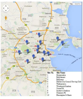
The sites at which the monitors are located are presented in Figure 1 where it can be seen that 138
there is good coverage of the central business district of Dublin. They are sited in a range of 139
different types of locations; some are close to multi-lane road arterials whereas others are 140
located in identified quiet areas. The data from the numbered sites on the figure are those 141
included in the analysis. 142
Location of Fig 1. 143
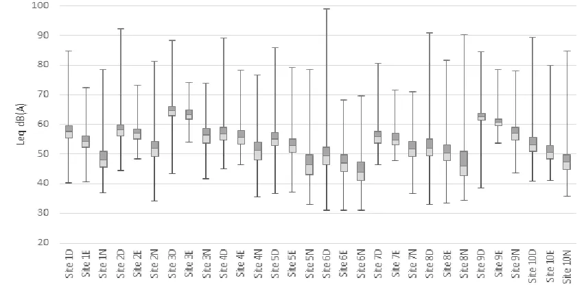
In Figure 2, the range of noise levels experienced across the sites is expressed in terms of LDAY, 144
LEVENING and LNIGHT where LDAY is the A-weighted long-term average sound level measured 145
between 19.00 and 23.00 and LNIGHT is the A-weighted long-term average sound level 147
measured between 23.00 and 07.00 (EU, 2002).All sites demonstrate the highest levels during 148
the day with levels reducing towards night, as expected. Also of note is the concentration of 149
the noise measurements close to the mean in most cases and also relatively high levels for sites 150
3 and 9 which are the sites located closest to multi-lane urban arterial roads. 151
Location of Fig 2 152
Central Statistics Census Database
153
The data used for the analysis on household transport characteristics are from the 2011 census 154
of Ireland (CSO, 2011). Some transport related questions are included in the census 155
questionnaire and they form the focus of this work. The questions include ‘how many cars 156
are in the household?’ and ‘what time do you start your trip to work?’ The data set includes 157
information on 1.7 million individual work trips made in 2011 and covers all those employed 158
in Ireland at the time of the census. The advantage of using the data is that it covers the 159
entire population and not just a sample. Work trips account for about a quarter of all trips 160
(CSO, 2011). For the research presented here, and in the absence of traffic data, the census 161
responses, in the areas in which noise monitors were placed in five sites in Dublin, were 162
analysed to see if there was a relationship between noise levels and three household 163
parameters 1) car ownership 2) the mode by which people travel to work in the area and 3) 164
the times at which people depart for work in the area. 165
Multinomial Logistic Regression
166
To address the second objective of the paper, multinomial logistic regression was used to 167
determine the relative importance of location, month of the year, weekday and hour of the 168
day on noise levels. Noise will vary depending on the level of each of those variables but it 169
flight paths or proximity to industry. In addition, it can be higher at different times of the day 171
typically during peak hours and it can also vary depending on the season. Multiple logistic 172
regression was used because it can analyse a mix of categorical and continuous variables in a 173
way that other regression techniques cannot. It can predict which of a number of categories a 174
variable can belong to given certain other information. Logistic regression can be used to 175
predict a categorical dependent variable on the basis of continuous and/or categorical 176
independents, to determine the effect size of the independent variables on the dependent and 177
to rank the relative importance of the independent variables. It applies maximum likelihood 178
estimation after transforming the dependent into a logit variable. The logit is a natural log of 179
the odds of the dependent variable equalling the highest value and in this way logistic 180
regression estimates the odds of a certain event occurring. The predictive success of the 181
logistic regression can be assessed by looking at the classification table, showing correct and 182
incorrect classifications of the dependent variable. Goodness of fit tests used are the 183
likelihood ratio test and the Nagelkerke statistic (Field, 2012). The logistic regression 184
equation is 185
𝑙𝑜𝑔𝑖𝑡(𝜋) = 𝑙𝑜𝑔𝑒( 𝜋
1 − 𝜋) = 𝑏0 + 𝑏1𝑋1+ 𝑏2𝑋2+ 𝑏3𝑋3+ 𝑏4𝑋4+ 𝑒
186
Where π= probability that the noise level falls in a particular Leq dBA band 187
b0 = intercept value, 188
b1, b2, etc = logistic regression coefficients 189
X1 = location (Site number), 190
X2 = hour of the day, 191
X3 = month 192
e = random error term 194
Whereas in linear regression the parameters are estimated using the method of least squares, 195
in logistic regression maximum-likelihood estimation is used. Parameters are estimated by 196
fitting models, based on the available predictors, to the observed data (Field, 2012). The 197
likelihood is a probability that the observed values of the dependent may be predicted from 198
the observed values of the independents. The log likelihood (LL) is its log and varies from 0 199
to minus infinity. LL is calculated in the modelling by iteration using maximum likelihood 200
estimation. Because -2LL has approximately a chi-square distribution, -2LL can be used for 201
assessing the significance of logistic regression. In general, as the model becomes better, the 202
-2LL will decrease in magnitude. 203
The independent variables were not chosen, as such, rather they were the only available 204
variables. To meet the non-metric dependent variable requirement of multinomial regression, 205
the noise measurements were discretised into 5dbA bandwidths. Variable definition and the 206
frequencies observed are shown in Table 1. The range of Leq dBA used was between 40 207
dBA and 75 dBA because the paucity of readings external to this range relative to the 208
numbers of readings within this range can be the source of irregularities in the model. 209
Results
210
The results section is divided in two parts. The first presents the results of the analysis which 211
examined the daily peak in morning noise levels to see if it is related to characteristics of 212
households in the area, such as, car ownership levels, the mode by which people travel to 213
work and work trip departure time. This section is subdivided into four sections 1) Peak 214
Period Noise Levels, Car Ownership Distribution, Mode used for Travel to Work and Time 215
of Departure to Work. The second part of the Results section presents the results of the 216
contribute most to noise levels: location, month of the year, weekday or hour of the day. This 218
section is divided into sub-sections each focusing on one of those variables. 219
Impact of Household Characteristics on Noise Levels
220
Peak Period Noise Levels 221
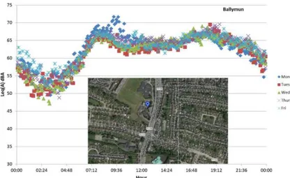
The first issue to be investigated was the cyclical daily profile evident for all sites, an 222
example of which for site 3 is presented in Figure 3. For this stage of the work, the focus was 223
centred on five sites, 1,3,4,5 and 9. 224
Location of Figure 3 225
In the absence of traffic measurements at the sites, the morning peak in noise levels was 226
investigated by exploring the peak hour trip characteristics of individuals living in the areas 227
under consideration using the 2011 census data (CSO, 2011). The characteristics considered 228
were the number of vehicles in households, the means by which individuals travelled to work 229
and what time individuals started their work trip. 230
Car Ownership Distribution 231
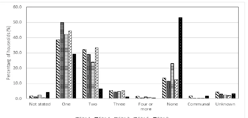
The first household characteristic to be examined was the distribution of car ownership, 232
presented in Figure 4. The largest difference between the areas appears to be for the 233
proportion of households that do not own a vehicle. Over 50% of the households in the Site 9 234
area do not own a vehicle followed by a much lower level in Site 3 at 23% and lower levels 235
again in the other areas. The Site 9 area has significantly lower numbers of 2 car households 236
than other areas at 6.4% compared with much higher levels for the other areas ranging to 237
24% in Site 3 area. For the one car households, there is also a wide degree of variation with 238
50% of households in Site 4 area owning one vehicle followed by Site 5 area at 45% and Site 239
cars in each of the areas examined are 7,699 in Site 1 area, 2,439 in Site 4 area, 12,014 in Site 241
3 area, 4,791 in Site 5 area and 2,449 in the Site 9 area. Normalised by population, these 242
figures translate to average car ownership levels of 0.83 cars per person in Site 1 area, 0.8 in 243
Site 4 area, 0.6 in Site 3 area, 0.73 in Site 5 area and 0.24 in the Site 9 area. When 244
comparing these levels with the morning noise level profiles presented in Figure 5, it would 245
appear that there is little impact of household car ownership levels on the noise levels shown. 246
Location of Figure 4.
247
Location of Figure 5 248
Mode used for Travel to Work 249
The modes by which individuals from the area travel to work was then examined, the results 250
of which are presented in Figure 6. Site 9 is very close to the city centre and so it is not 251
surprising that a large proportion (44.8%) of individuals walk to work. Sites 1 and 3 also 252
show significant numbers walking to work at 26% and 23.6% respectively. Significant 253
proportions of individuals drive to work in all areas (28%-40.7% with the highest level 254
reports in Site 4, followed by Sites 5, 1 and 3) except in the case of the Site 9 area. Again, 255
there is little evidence of noise levels being related to the numbers of people driving to work 256
from those locations. 257
Location of Figure 6. 258
Time of Departure to Work 259
The last characteristic to be examined was the time of departure for work/school/university 260
trip. All work trips in the areas are included initially and the results are normalised by 261
population of area and presented in Figure 7. When answering the question in the census, 262
time band are plotted mid-way through that time band on the figure, and with reference to the 264
secondary right hand axis, for the purposes of relating the results to the noise levels in the 265
areas which are also plotted in Figure 7. The noise results plotted are the average of five 266
weekdays and they are referenced to the primary left hand axis. 267
There would appear to be a strong trend between the rising noise levels in the morning peak 268
period for all areas with the numbers departing for work during that period but the noise 269
levels generated do not correspond quantitatively with the numbers departing in each area. 270
For example, the noise levels in Site 3 (Ballymun) are higher than in other areas but other 271
areas have higher numbers departing for work relative to population during the period. It is 272
likely that the proximity of the noise monitor to a major road in Ballymun (see Figure 3) is 273
dominating the measurements at this site. The relationship is less clear on the back side of 274
the curve but, in any case, both noise and work trip departures drop during this time period. 275
Also of note from Figure 7, is the similar rate of increase of noise levels from 4:00am to 276
8:00am regardless of noise level starting point at 4:00am. 277
Figure 8is similar to Figure 7 but this time only those who commute by car are included 278
when looking at the departure time. Again there is a notable upward trend between rising 279
noise levels and the numbers departing for work by car but no distinguishable relationships 280
between the actual numbers departing and the noise levels in the area. It can be concluded, 281
therefore, that the numbers departing for work in an area in the morning peak period 282
contribute to the ambient noise levels in an area but it is unlikely that this characteristic is 283
more important than proximity to major noise sources. 284
Location of Figure 7. 285
Location of Figure 8. 286
Multinomial Logistic Regression Model Results
288
Before including variables in the model, a test for collinearity between them was completed, 289
the results of which are shown below in Table 2. The collinearity diagnostic results show that 290
no independent variables have excessively high proportions on small eigenvalues indicating 291
that collinearity between the variables is not an issue. (Field, 2012). 292
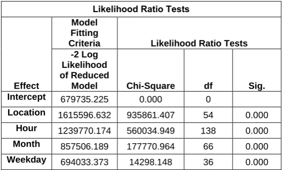
An overall check on the relationship between the dependent and independent variables is the 293
significance for the final model chi-squared value, after the independent variables have been 294
added, the results of which are shown in Table 3 where significance is shown. The reduction 295
in -2LL value for the final model with the independent variables included compared with the 296
model without them can also be seen in Table 3, another indicator that the addition of the 297
independent variables improves the model. The overall Nagelkerke statistic value was 0.744 298
representing relatively decent sized effects (Field, 2012). Another useful measure to assess 299
the utility of the model is classification accuracy which compares the predicted group 300
membership based on the logistic model with the actual. The benchmark used here is that the 301
model is considered useful if it shows a 25% improvement over the rate of accuracy achievable 302
by chance alone. The proportional by chance accuracy was computed by calculating the 303
proportion of cases for each group based on the number of cases in each group for the 304
dependent variable in Table 1 and then squaring and summing the proportion of cases in each 305
group; the result of which was calculated to be 0.22. The proportional by chance accuracy 306
criteria therefore = 1.25*0.22 = 27%. The classification accuracy rate from the model was 307
calculated to be 58.6% from Table 4 below indicating that the model can be characterised as 308
useful. It can be seen in Table 5 that all independent variables included are significant and 309
therefore add to the model. For the variables, the larger the chi-square value, the greater the 310
the greatest loss of model fit, followed by hour of the day, month and weekday. This table 312
therefore gives an indication of the ranking of the independent variables. 313
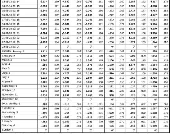
The model parameter estimates are presented in Table 6. The table includes the Beta (B) 314
coefficients for each noise band and they correspond to the weight of each of the independent 315
variables on the utility function. The corresponding standard errors, which should be less than 316
2, are also shown. Statistical significance to the 0.01 level is shown with bold font, to the 0.05 317
level with italic font and no statistical significance is shown with normal font. The reference 318
value for the dependent variable is the noise band level 70-74.99 dBA and the reference values 319
for each of the independent variables are Site 10 (Blessington St Basin) for location, 23:00-320
23:59 for hour of the day, December for month and Sunday for day of the week. 321
Model Results for the Location Variable 322
Examining, in the first instance, the impact of location on noise level, the model results for 323
location 6 (Woodstock Gardens) are positive for all noise band levels and have higher absolute 324
values for the lower noise bands when compared with noise levels at location 10 (Blessington 325
St Basin), the reference location. The highest value of 6.06 for band 40-45 dBA indicates noise 326
levels at that location are more likely to be in that band than others, followed by bands 45-327
49.99 (4.8) and 50-54.99 (3.3) with a reduction in likelihood of measurements in the higher 328
noise band levels. In most of the other locations, negative B values in the lower band levels 329
indicate that noise levels in those locations are less likely to be in the lower noise bands 330
compared with location 10. This is particularly the case for Ballymun (location 3) and 331
Chancery Park (location 9); both noise monitors in these two locations being close to heavily 332
trafficked arterial roads. The negative coefficients dominate for the three lower noise band 333
levels but for those bands above 55 dBA most of the coefficients are positive indicating higher 334
Ballyfermot (site 2), noise levels are more likely to be in the band 60-64.99 (2.07) and in 336
Ballymun (site 3) in band 65.99-70 (5.54) compared with location 10. 337
Model Results for Hour of the Day Variable 338
The next variable examined was the hour of the day and a definite pattern emerges when 339
examining the coefficients. During night time hours from 00:00 to 05:59, there is a higher 340
likelihood for noise levels during those hours to be in the lower noise band levels compared 341
with noise levels in the hour 23:01-23:59 (the reference hour) e.g. 02:00-02:59 has the highest 342
B value of 3.783 for noise band 40-44.99 indicating that during that hour, noise levels are most 343
likely to be in that band and noise levels least likely to be in the 60-64.99 band (-2.591). For 344
daytime hours, the trends in the B coefficients change. High negative values now appear in the 345
lower noise band levels and high positive values in the higher bands when comparing the noise 346
levels to those in the hour 23:01-23:59. For example, in the case of 09:00-09:59, noise levels 347
in the 40-44.99 band level are the least likely (-6.154) and are most likely to be in the 65-69.99 348
band (3.977). This pattern in coefficients is repeated for all hours of the day up until 21:59. 349
Model Results for the Month Variable 350
Looking at the next variable, the month in which the noise measurements are taken, in the case 351
of January, the coefficients are similar across most noise bands with the lower bands having 352
marginally higher coefficients indicating that there is a higher likelihood of noise 353
measurements falling in those bands when compared with December (the reference case). In 354
the case of June, there is a much higher likelihood that noise levels will be in the 40-44.99 dBA 355
band (5.791) than other noise bands and least likely to be in the 56-69.99 band (-1.416) when 356
compared to December. Similar spreads of coefficients are shown for July and August. In 357
October and November, again the likelihood of measurements falling in the lower noise bands 358
Model Results for Day of the Week Variable 360
When examining the last independent variable in the model, day of the week, the following 361
trends were found. For all days of the week, noise measurements are most likely to be in the 362
higher noise level bands and less likely to be in the lower noise bands compared with Sunday. 363
For example, the coefficients for the 60-64.99 and 65-69.99dBA bands for Thursday are 0.413 364
and 1.191 respectively compared with -0.475 and -0.906 for the 40-44.99 and 45-49.99 dBA 365
bands respectively. All coefficients for all days in the upper bands are significant to the 0.01 366
level but there is no significance for some noise bands in the case of Monday, Tuesday and 367
Friday. 368
Discussion
369
In addressing the first objective of the paper i.e. to determine if household transport 370
characteristics have an influence on urban noise levels, the findings suggest that proximity to 371
transport arteries have more influence on noise level than household car ownership, the mode 372
by which people travel to work and their work trip departure time. While the exploration of 373
the data in this way might not appear fruitful in the context of the findings, it does indicate for 374
local authorities that areas that are not close to transport arteries but perhaps do have high car 375
ownership and usage levels, could still be considered as possible candidates for designation as 376
‘quiet areas’ (EU, 2002) as opposed to the more anecdotal approach that a ‘quiet area’ would 377
include a park or a pedestrianised area. Another useful finding for local authorities from this 378
part of the paper, is that, while there was no clear relationship between the numbers of car users 379
or all commuter numbers departing for their work trip in the morning peak period and the noise 380
levels in that area, there was a highly similar rate of increase in noise levels in the morning 381
for the morning peak period at sites which do not have noise long-term monitoring facilities 383
available. 384
The second part of the paper examined the contribution that a number of variables make to 385
noise levels: location, hour of the day, month and weekday. This piece of work attempted to 386
address a gap Zuo et al (2014) had identified in that they found that location (spatial) aspects 387
of a site were the most important variable in defining noise levels but were less confident in 388
their assessment of temporal variables because of limitations on their data collection that meant 389
peak hour levels were not captured. The research presented here took particular advantage of 390
having a continuous profile of noise measurements over a year and therefore having detailed 391
information about noise level measurements at all times of the day. This enabled three levels 392
of temporal variables along with location to be examined very comprehensively. From Table 393
5, it can be seen that the results here support the findings of Zuo et al (2014) i.e. that location 394
contributes most to noise levels followed by the hour of the day, month and weekday in that 395
order with weekday contributing very little. The findings also agree with those of Torija et al 396
(2010) which suggested that the addition of temporal variables improves noise level prediction. 397
The findings are useful in the context of how local authorities might allocate limited resources 398
to the measurement of noise. Measuring noise levels at different locations for a day is likely 399
to generate the most benefit in terms of noise level prediction as location and hour of the day 400
were two variables identified as contributing most to the noise levels. Trying to determine 401
seasonal variation (difference between months) or weekday variation is less useful in 402
contributing to noise level predictive capacity. 403
Conclusions
404
There would appear to be no correlation between household car ownership levels in an urban 405
departing from work in an area. There would appear to be a strong trend between the rising 407
noise levels in the morning peak period for all areas with the numbers departing for work 408
during that period but the noise levels generated do not correspond quantitatively with the 409
numbers departing in each area. Again there is a notable upward trend between rising noise 410
levels and the numbers departing for work by car but no distinguishable relationships 411
between the actual numbers departing and the noise levels in the area. It can be concluded 412
that the numbers departing for work in an area in the morning peak period contribute to the 413
ambient noise levels in an area but it is unlikely that this characteristic is more important than 414
proximity of the monitor to major noise sources. 415
The multinomial logistic regression model developed to predict noise levels using the 416
independent variables of location, month, weekday and hour of the day can be considered 417
useful in that it can be seen from the -2LL test that the independent variables all make a 418
significant contribution. Having said that, the model is far from perfect in that it predicts 419
correctly 58.5% of the time although this is considerably higher than the 27% proportional by 420
chance accuracy. The results show that location is the most important of the variables followed 421
by hour of the day, and then month, with day of the week offering the least contribution in 422
terms of predictive capacity. 423
Previous work had raised a question about how temporal variables contribute to urban noise 424
levels. The research addresses this question whereby it notes that the time of day contributes 425
significantly to noise level prediction but not as much as spatial variables. It also finds that 426
monthly and weekday influenced variations contribute less in terms of predictive contribution. 427
Measuring noise levels at different locations for a day is likely to generate the most benefit in 428
terms of the optimum use of noise level measurement resources as location and hour of the day 429
seasonal variation (difference between months) or weekday variation is less useful in terms of 431
their contribution to noise level prediction. 432
ACKNOWLEDGEMENTS 433
The authors would like to thank Dublin City Council for the use of the data. 434
REFERENCES 435
Camusso, C. (2007). A methodology to cluster urban sections for the definition of new noise 436
indicators to monitor the acoustical climate of urban areas. Proceedings of the ECTRI Young 437
Researchers Seminar, Brno, Czechoslovakia 438
Central Statistics Office (2011). Census of Ireland 2011, Central Statistics Office, Ireland. 439
European Union (2002). Directive 2002/49/EC of the European Parliament and of the 440
Council of 25 June 2002 relating to the assessment and management of environmental noise. 441
2002. Brussels. http://ec.europa.eu/environment/noise/directive.htm Accessed 12/02/2015 442
Field, A. (2013). Discovering Statistics using IBM SPSS Statistics. 4th Edition, Sage 443
Publications Ltd. London. 444
Geraghty, D., McDonald, P., Humphreys, I. and O’Mahony, M. (2015). Design and 445
operational characteristics of a noise monitoring network in Dublin, Ireland. Procs of the 94th 446
Annual Meeting of the Transportation Research Board, Washington DC, January 2015. 447
Halperin, D. (2014). Environmental noise and sleep disturbances: A threat to health? Sleep 448
Science 7, 209-212. 449
IEC (2013). International Electrotechnical Commission. Electroacoustics – Sound Level 450
Meters Tests. IEC 61672. 451
Koushki, P., Cohn, L., and Felimban, A. (1993). ”Urban Traffic Noise in Riyadh, Saudi 453
Arabia: Perceptions and Attitudes.” J. Transp. Eng., 119(5), 751–762. 454
Lavandier, C. and Delaitre, P. (2015). Individual and shared representations on “zones 455
calmes” (“quiet areas”) among the French population in urban context. Applied Acoustics, 456
99, 135-144. 457
Mateus M., Dias Carrilho, J.A., Gameiro da Silva, M.C. (2015). Assessing the influence of 458
the sampling strategy on the uncertainty of environmental noise measurements through the 459
bootstrap method. Applied Acoustics 89, 159–165. 460
Mehdi, M.R., Kim, M., Seong, J.C., and Arsalan, M.H. (2011). Spatio-temporal patterns of 461
road traffic noise pollution in Karachi, Pakistan, Environment International 37. 97–104 462
Silva, L.T., Oliveira, M. and Silva, J.F. (2014). Urban form indicators as proxy on the noise 463
exposure of buildings. Applied Acoustics, 76, 366-376. 464
Sonitus Systems. (2014). Noise monitoring web-based interface. 465
http://www.sonitussystems.com/ Accessed 13/02/2015. 466
Sygna, K., Aasvang, G.M. Aamodt, G., Oftedal, B., and Krog, N.H. (2014). Road traffic 467
noise, sleep and mental health. Environmental Research 131, 17–24 468
Tobías, A. Recio, A., Díaz, J. and Linares, C. (2015). Health impact assessment of traffic
469
noise in Madrid (Spain) Environmental Research 137. 136–140 470
Torija, A.J.,Genaro, N., Ruiz, D.P., Ramos-Ridao, A., Zamorano, M. and Requena, I. (2010). 471
Priorization of acoustic variables: Environmental decision support for the physical 472
characterization of urban sound environments, Building and Environment 45, 1477-1489. 473
Weber, N., Haase, D. and Franck, U. (2014). Traffic-induced noise levels in residential urban 474
Zuo, F., Y. Li, S. Johnson, J. Johnson, S. Varughese, R. Copes, F. Liu, H.J. Wu, R. Hou and 476
H. Chen, H. (2014). Temporal and spatial variability of traffic-related noise in the City of 477
Toronto, Canada. Science of the Total Environment. Vol. 472. pp 110-1107. 478
479
LIST OF FIGURES 480
481
Fig 1. Locations of noise monitors in Dublin 482
Fig. 2. Boxplots of LDAY, LNIGHT, and LEVENING for each site 483
Fig.3. Daily cyclical profiles of noise measurements for site 3, Ballymun 484
Fig. 4. Household car ownership distribution 485
Fig.5. Morning noise measurement profiles 486
Fig. 6. Modes by which people travel to work 487
Fig. 7. Numbers departing for work normalised by population with weekday morning noise 488
profile. 489
Fig 8. Numbers of car commuters departing for work normalised by population with weekday 490
morning noise profiles. 491
492
493
494
495
496
497
498
500
Variable Definition and Frequencies
Variable Definition N % Notes
Dependent variable Leq dBA 45.00 73,465 7.3%
50.00 170,390 16.9%
55.00 293,028 29.1%
60.00 282,115 28.0%
65.00 151,229 15.0%
70.00 34,564 3.4%
75.00 2,867 0.3% Reference Category
Independent Variable 1: Location 1.00 103,307 10.3%
2.00 103,309 10.3%
3.00 102,392 10.2%
4.00 100,630 10.0%
5.00 100,211 9.9%
6.00 96,839 9.6%
7.00 101,298 10.1%
8.00 95,081 9.4%
9.00 103,752 10.3%
10.00 100,839 10.0% Reference Category
Independent Variable 2: Hour 1 38,328 3.8%
2 40,717 4.0%
3 39,736 3.9%
4 39,865 4.0%
5 40,722 4.0%
6 41,711 4.1%
7 42,387 4.2%
8 42,571 4.2%
9 42,548 4.2%
10 42,546 4.2%
11 42,506 4.2%
12 42,525 4.2%
13 42,680 4.2%
14 42,690 4.2%
15 42,679 4.2%
16 42,708 4.2%
17 42,696 4.2%
18 42,704 4.2%
19 42,710 4.2%
20 42,701 4.2%
21 42,654 4.2%
22 42,605 4.2%
23 42,443 4.2%
24 42,226 4.2% Reference Category
Independent Variable 3: Month 1 85,229 8.5%
2 73,026 7.2%
3 83,597 8.3%
4 82,330 8.2%
5 86,908 8.6%
6 82,670 8.2%
7 84,745 8.4%
8 85,275 8.5%
9 83,671 8.3%
10 88,176 8.8%
11 83,893 8.3%
12 88,138 8.7% Reference Category
Independent Variable 4: Weekday 1 144,397 14.3%
2 142,237 14.1%
3 142,729 14.2%
4 142,225 14.1%
5 144,598 14.3%
6 146,757 14.6%
7 144,715 14.4% Reference Category
Total 1,007,658 100.0%
[image:22.595.124.474.89.721.2]501
503
504
Collinearity Diagnostics
Eigenvalue
Condition Index
Variance Proportions
Dimension (Constant) Location Hour Weekday Month
1 4.305 1.000 .00 0.01 0.01 0.01 0.01
2 .224 4.379 .00 0.16 0.75 0.03 0.07
3 .215 4.472 .00 0.44 0.01 0.00 0.56
4 .205 4.578 .00 0.17 0.02 0.68 0.13
5 .050 9.279 1.00 0.23 0.22 0.28 0.24
[image:23.595.83.511.117.252.2]505
Table 2. Collinearity diagnostics 506
507
508
509
510
511
512
513
514
515
516
517
518
519
520
521
522
523
524
525
526
Model
Model Fitting
Criteria Likelihood Ratio Tests
-2 Log
Likelihood Chi-Square df Sig.
Intercept Only 1943545.339
[image:24.595.139.459.88.189.2]Final 679735.225 1263810.113 294 .000
Table 3. Model Fitting Information 528
529
530
531
532
533
534
535
536
537
538
539
540
541
542
543
544
545
546
547
548
549
550
551
552
Classification
Observed Leq dBA
Predicted Leq dBA
45.00 50.00 55.00 60.00 65.00 70.00 75.00 Percent Correct 45.00
32539 34977 5651 286 12 0 0 44.3%
50.00
15944 77229 72928 4283 5 1 0 45.3%
55.00
3556 36674 178013 74446 330 9 0 60.7%
60.00
382 5176 62621 196809 17038 89 0 69.8%
65.00
112 1148 7609 43447 92988 5925 0 61.5%
70.00
43 411 2115 3631 15799 12565 0 36.4%
75.00
3 458 990 775 440 201 0 0.0%
Overall Percentage
5.2% 15.5% 32.7% 32.1% 12.6% 1.9% 0.0% 58.6%
[image:25.595.72.524.71.297.2]554
Table 4. Classification Table. 555
556
557
558
559
560
561
562
563
564
565
566
567
568
569
570
571
572
573
575
Likelihood Ratio Tests
Effect
Model Fitting
Criteria Likelihood Ratio Tests -2 Log
Likelihood of Reduced
Model Chi-Square df Sig. Intercept 679735.225 0.000 0
Location 1615596.632 935861.407 54 0.000
Hour 1239770.174 560034.949 138 0.000
Month 857506.189 177770.964 66 0.000
Weekday 694033.373 14298.148 36 0.000
[image:26.595.158.439.91.259.2]576
578
Parameter Estimates
Leq dBA
40-44.99 45-49.99 50-54.99 55-59.99 60-64.99 65-69.99
B SE B SE B SE B SE B SE B SE
Intercept 4.145 .172 6.763 .169 6.840 .169 4.796 .168 .535 .170 -3.571 .190
LOCATION: Drumcondra: 1 -1.461 .102 -1.263 .101 -.631 .100 1.204 .100 1.548 .102 .549 .111
Ballyfermot: 2 -4.749 .107 -3.249 .103 -1.196 .102 1.447 .102 2.072 .103 .754 .112
Ballymun: 3 11.534 - .162 -7.928 .106 -4.542 .103 -.246 .102 4.145 .104 5.538 .108
Chapelizod Rd: 4 -3.153 .123 -2.001 .120 -.213 .120 1.807 .120 2.147 .121 .805 .131
Walkinstown: 5 -.686 .086 -1.271 .084 -.742 .084 .265 .084 -.042 .086 .141 .094
Woodstock Gdns: 6 6.602 .323 4.806 .323 3.305 .323 2.259 .323 1.799 .325 1.157 .336
Navan Rd: 7 -2.573 .203 -.602 .200 1.506 .200 3.035 .200 2.634 .201 1.305 .210
Irishtown: 8 -.652 .073 -1.298 .071 -1.631 .070 -1.841 .071 -1.721 .074 -1.388 .083
Chancery Pk: 9 13.179 - .277 -8.939 .106 -4.713 .099 .101 .098 3.928 .099 3.150 .104
Blessington St: 10 0b 0b 0b 0b 0b 0b
HOUR: 00:00-00:59: 1 1.219 .188 .715 .187 .337 .186 -.096 .186 -1.188 .188 -.740 .218
01:01-01:59: 2 2.778 .183 1.757 .181 .927 .181 -.356 .180 -2.063 .184 -1.307 .217
02:00-02:59: 3 3.783 .178 2.394 .177 1.074 .177 -.690 .176 -2.591 .181 -1.173 .208
03:00-03:59: 4 3.486 .171 2.140 .170 .826 .169 -.873 .169 -2.920 .175 -1.475 .203
04:00-04:59: 5 3.072 .181 2.017 .180 .994 .180 -.402 .179 -2.615 .185 -1.200 .213
05:00-05:59: 6 1.015 .168 .510 .166 -.033 .166 -.577 .165 -2.075 .168 -1.377 .200
06:00-06:59: 7 -1.610 .169 -1.156 .167 -.882 .167 -.525 .166 -.144 .168 .148 .193
07:00-07:59: 8 -4.094 .173 -2.759 .170 -1.632 .169 -.339 .169 1.584 .170 3.510 .188
08:00-08:59: 9 -4.992 .166 -3.687 .163 -2.279 .162 -.552 .162 1.847 .163 4.355 .180
09:00-09:59: 10 -6.154 .163 -4.394 .158 -2.541 .157 -.794 .157 1.707 .158 3.977 .176
10:00-10:59: 11 -6.302 .168 -4.306 .161 -2.321 .160 -.636 .160 1.994 .161 3.949 .179
11:00-11:59: 12 -7.022 .166 -4.874 .158 -2.646 .156 -.834 .156 1.891 .157 3.875 .175
13:01-13:59: 14 -6.637 .169 -4.530 .162 -2.396 .161 -.524 .160 2.184 .162 4.317 .179
14:00-14:59: 15 -6.393 .171 -4.444 .165 -2.309 .163 -.378 .163 2.389 .164 4.668 .182
15:01-15:59: 16 -6.146 .173 -4.249 .167 -2.200 .166 -.272 .165 2.414 .167 4.763 .183
16:01-16:59: 17 -5.785 .172 -4.098 .167 -2.200 .166 -.272 .166 2.320 .167 4.947 .183
17:01-17:59: 18 -5.447 .170 -4.034 .166 -2.251 .165 -.372 .165 2.352 .166 5.013 .183
18:01-18:59: 19 -5.100 .176 -3.687 .172 -1.955 .171 -.109 .171 2.429 .172 5.174 .188
19:01-19:59: 20 -4.994 .171 -3.598 .168 -1.894 .167 -.291 .166 1.933 .168 4.270 .185
20:01-20:59: 21 -4.384 .170 -3.146 .167 -1.631 .166 -.438 .166 1.529 .168 3.390 .185
21:01-21:59: 22 -3.019 .180 -2.110 .177 -.981 .177 -.258 .176 1.323 .178 2.159 .197
22:01-22:59: 23 -1.499 .184 -1.011 .183 -.496 .182 -.206 .182 .671 .183 .644 .207
23:01-23:59: 24 0b 0b 0b 0b 0b 0b
MONTH: January: 1 1.111 .107 1.357 .103 1.145 .102 1.018 .102 .918 .103 .678 .105
February: 2 -1.487 .076 -1.182 .071 -.910 .069 -.674 .068 -.393 .069 -.343 .072
March: 3 2.592 .118 2.393 .116 1.783 .115 1.106 .115 .345 .115 .118 .118
April: 4 -.680 .070 -.718 .065 -.678 .063 -1.170 .063 -1.674 .064 -1.664 .068
May: 5 2.111 .102 1.750 .099 1.661 .097 .586 .097 -.415 .098 -1.465 .103
June: 6 5.791 .170 4.278 .169 3.152 .168 1.520 .168 .200 .169 -1.418 .173
July: 7 6.018 .122 4.096 .120 2.594 .119 .331 .119 -.950 .120 -2.793 .126
August: 8 6.101 .152 4.381 .151 3.068 .150 1.207 .150 -.211 .151 -1.998 .156
September: 9 5.062 .138 3.578 .137 2.519 .136 1.171 .136 .027 .137 -.769 .140
October: 10 2.646 .092 1.945 .089 1.158 .088 .311 .088 -.612 .089 -.674 .092
November: 11 2.916 .108 2.267 .106 1.456 .105 .938 .105 .123 .106 .028 .108
December: 12 0b 0b 0b 0b 0b 0b
DAY: Monday: 1 .288 .083 -.019 .082 .015 .081 .196 .081 .772 .082 1.187 .086
Tuesday: 2 .299 .080 -.113 .078 -.185 .078 -.081 .078 .603 .079 1.097 .083
Wednesday: 3 -.183 .073 -.714 .072 -.787 .071 -.529 .071 .196 .072 1.038 .076
Thursday: 4 -.475 .075 -.906 .073 -.819 .072 -.457 .072 .413 .073 1.191 .077
Friday: 5 -.862 .073 -1.057 .071 -.983 .070 -.560 .070 .376 .071 1.267 .075
Saturday: 6 -.506 .082 -.304 .081 -.154 .080 .126 .080 .610 .081 1.089 .085
[image:28.842.72.620.74.505.2]Sunday: 7 0b 0b 0b 0b 0b 0b
580
581
[image:29.842.70.400.89.485.2]582
584
585
[image:30.842.75.502.99.310.2]586
Figure 2. Boxplots of Lday, Levening and Lnight for each site 587
589
Figure 3. Daily cyclical noise measurement profiles for Site 3 590
592
[image:32.842.76.510.69.276.2]593
Figure 4. Car ownership of households 594
596
[image:33.842.66.506.73.355.2]597
Figure 5. Morning peak noise profile 598
600
[image:34.842.68.503.74.292.2]601
Figure 6. Modes by which people travel to work 602
604
[image:35.842.58.501.69.368.2]605
Figure 7. Numbers departing for work in an area with weekday morning noise profile 606
608
Figure 8. Numbers of car commuters departing for work in an area with weekday morning noise profile 609
610