A theory of system behaviour in the presence of node and link failure

A Theory of System Behaviour in the Presence of

Node and Link Failure

Adrian Francalanza

, Matthew Hennessy

Abstract

We develop a behavioural theory of distributed programs in the presence of failures such as nodes crashing and links breaking. The framework we use is that of Dπ, a language in which located processes, or agents, may migrate between dynamically created locations. In our extended framework, these processes run on a distributed network, in which individual nodes may crash in fail-stop fashion or the links between these nodes may become perma-nently broken. The original language, Dπ, is also extended by a ping construct for detecting and reacting to these failures.

We define a bisimulation equivalence between these systems, based on labelled actions which record, in addition to the effect actions have on the processes, the effect on the actual state of the underlying network and the view of this state known to observers. We prove that the equivalence isfully abstract, in the sense that two systems will be differentiated if and only if, in some sense, there is a computational context, consisting of a surrounding network and an observer, which can see the difference.

Key words:

distributed calculi, node and link failure, reduction barbed congruence, labelled transition systems, bisimulation

1 Introduction

• formalise a simple framework, a distributed process calculus, for describing computations over a distributed network in which individual nodes and links

between the nodes are subject to failure

• use this framework to develop a behavioural theory of distributed systems in which these failures are taken into account.

Our point of departure is Dπ [20], a simple distributed version of the standardπ -calculus [27], where the locations that host processes model closely physical net-work nodes. Ignoring the type system developed for Dπ, which is orthogonal to the issues addressed here, we consider the following three abstract server implementa-tions as motivation:

server ⇐ (νdata)          

l[[req?(x,y).data!hx,yi]]

|l[[data?(x,y).y!hf(x)i]]          

servD ⇐ (νdata)          

l[[req?(x,y).gok1.data!hx,yi]] |k1[[data?(x,y).gol.y!hf(x)i]]          

servD2Rt⇐ (νdata)                                  l                                  

req?(x,y).(νsync)                 

gok1.data!hx,synci

|gok2.gok1.data!hx,synci |sync?(x).y!hxi

                                                  

|k1                    

data?(x,y).          

gol.y!hf(x)i

|gok2.gol.y!hf(x)i                                                               

The three systemsserver, servDandservD2Rtimplement a server that accepts a single request for processing on channelreqat locationlwith two arguments,xthe value to be processed andythe return channel on which to return the result of the processing. A typical client for these servers would have the forml[[req!hn,reti]], sending the namenas the value to be looked up andretas the return channel.

Every server forwards the request to an internal database hidden from the client, denoted by the scoped channeldata, which processes the value using an unspecified function f(x). The three implementations differ by where the internal database is located and how it is handled. More specifically,serverholds the databaselocallyat

intermediary nodek2 and non-deterministically selects one of two results if both routes are active.

Intuitively, these three server implementations are not equivalent because they ex-hibit distinct behaviour in a setting with node and link failure. For instance, if node

k1 fails, servD and servD2Rt may not be able to service a client request whereas server would continue to work seamlessly. Moreover, servD and servD2Rt are also distinct because if the link betweenlandk1breaks,servDmay block and not serve a request while servD2Rtwould still operate as intended. Despite the fact that these three implementations are qualitatively different, it is hard to distinguish between them in Dπtheories such as [18].

In this paper, we develop a behavioural theory that tells these three systems apart. We use extended Dπconfigurations of the formΣ.NwhereΣis a representation of the current state of the network, andNconsists of the systems such as those we have just seen, that is software executing in a distributed manner overΣ. HereΣrecords the set of nodes in the network, theirstatus(whether they are aliveor dead), and theirconnectivity(the set of symmetric links between these nodes). This results in a succinct but expressive framework, in which many of the phenomena associated with practical distributed settings, such as routing algorithms and ad-hoc network discoveries, can be examined.

The corresponding behavioural theory takes the form of(weak) bisimulation equiv-alence, based on labelled actions

Σ.N −→µ Σ0.N0 (1)

where the labelµrepresents the manner in which an observer, also running on the networkΣ, can interact with the systemN. This interaction may not only change the state of the system, to N0, in the usual manner, but also affect the nature of the underlying network. For instance, an observer may extend the network by creating new locations or otherwise induce faults in the network by killing sites or breaking links between sites, thereby capturing at least some of the reaction ofNto dynamic failures.

Table 1.Syntax of typed DπF

Types

T,U,W ::= ch | loc[S,C] S ::= a | d C,D ::= {u1, . . . ,un} Processes

P,Q ::= u!hVi.P |u?(X).P | ∗u?(X).P |ifv=uthenPelseQ |0 |P|Q |(νn:T)P

| gou.P |kill |breaku |pingu.PelseQ

Systems

M,N,O ::= l[[P]] |N|M |(νn:T)N

The paper is organised as follows: Section 2 introduces our language, DπF, its re-duction semantics and a corresponding contextual equivalence, based on the notion of reduction barbed congruence of Honda et al [22]. In Section 3 we present an initial definition of actions for DπF, based on the general approach of [19]. The resulting bisimulation equivalence can be used to demonstrate equivalences be-tween systems, but we show, by a series of examples, that it is too discriminating. In Section 4 , we revise the definition of these actions, by abstracting from internal information present in the action labels, and demonstrate, through a series of exam-ples, that the resulting bisimulation equivalence corresponds, in some sense, to the contextual equivalence defined earlier in Section 2. Finally, in Section 5, we state and prove the main result of the paper, that is that the refined bisimulation is indeed

fully abstract with respect to aforementioned contextual equivalence; this means that two systems will be differentiated by the bisimulation equivalence if and only if, in some sense, there is a computational context, consisting of a network and an observer, which can see the difference. Section 6 concludes with an overview of related work and future directions.

2 The language

We assume a set of variables V, ranged over by x,y,z, . . . and a separate set

ofnames, N, ranged over byn,m, . . ., which is divided into locations, L,

ranged over byl,k, . . .and channels, C, ranged over bya,b,c, . . .. Finally we

use u,v, . . . to range over the set of identifiers, consisting of either variables and names.

with a rich type system for regulating access control. Since this is orthogonal to our concerns we ignore this type system. Instead we use a very simple notion of type, which simply records the proposed use of an identifier. Thus, ifnis used as a channel inN, then Tis simplych; however if it is a location thenT = loc[S,C] records it’sstatus S, whether it is alive a or deadd, and the set of locationsC to which it is linked, {l1, . . . ,ln}. Note that theseT should not be considered asstatic

types; in particular, as a computation proceeds, the status and connectivity of loca-tions may change. Another change from the original Dπis that we do not speficy the location where a channel can be used; here a channel can be used at any location.

The syntax for agents,P,Q, is an extension of that in Dπ. There are input and output on channels; hereVis a tuple of identifiers, andXa tuple of distinct variables, to be interpreted as a pattern. We also have the standard forms of parallel, replicated in-put, local declarations, a test for equality between identifiers and an asynchronous migration construct. As we shall see once we introduce the reduction semantics of this language, migration under failure assumes a different semantics from that in the original Dπ, but its characteristic asynchrony is still preserved in our language. Pro-cesses are also extended with a a conditional ping construct,l[[pingk.PelseQ]], in the style of [2,1,26], branching tol[[P]] orl[[Q]] depending on theaccessibilityofk

froml. It acts as a form of perfect failure detector [5], the implementation of which typically necessitates tighter synchronisation between locations. Despite this appar-ent limitation1_{, the ping construct still describes the asynchrony between network} failure and failure discovery/detection as two distinct and independent events. To-gether, the ping and asynchronous migration operations give a programming level of abstraction close an idealised form of the IP/ICMP layers in the Internet protocol suite[23]. The semantics of new location process is also different from that of Dπ, since it is subject to restrictions imposed by the present state of the network as well. In particular, new locations can only short-circuit paths of connections between lo-cations but cannot provide a new path for two unreachable nodes. Finally, we have two new constructs to simulate failures in the style of [26];l[[kill]] kills the location

l, whilek[[break l]] breaks the link betweenl andk, if it exists. We are not really interested in programming with these last two operators. Nevertheless, when we come to considercontextual behaviour, their presence will mean that the behaviour will take into account the effects ofdynamicfailures.

We relegate the standard notions of free and bound occurrences of both names and variables to the appendix (see Section A) and assume the associated concepts of α-conversion and substitution; see [27,17] for similar definitions. It is worth emphasising that location names, and indeed identifiers, may occur in types, and this must be taken into account when these concepts are defined. Furthermore, we

will assume that channel communication is well-sorted (for any outputa!hVi.Pand inputa?(X).Qon any channela, we have|V|= |X|) that all system terms areclosed, that is they have no free occurrences of variables.

Network representations: Reductions of systems are defined with respect to a network representation, ∆, describing the current state of the network. Intuitively ∆records the set of locations in existence, whether they are alive or dead, and any live links between them.

Definition 1 (Link sets) Any binary relation L over the set of locations L is called a linkset. We use dom(L) to denote its domain, that is the collection of locations l such thathl,ki ∈ L, for some k.

A linkset is meant to represent both location liveness and a collection of symmetric linksbetween locations. Specifically we writeL `l:alivewheneverhl,li ∈ Land

L `l↔k whenever

• hl,ki ∈ L • orhk,li ∈ L.

The reflexive interpretation of link-sets expresses liveness and at the same time permits the smooth handling of the degenerate case of a process moving from a site

ltolitself.

Definition 2 (Components) A subset K of a linkset L is called a component, if all locations inK are mutually accessible; that is, using the obvious notation,L `

k1↔∗k2for every k1,k2 ∈ K. Every location l∈dom(L), generates a component: [l]L= {hk1,k2i ∈ L | L `l↔∗k1 orL `l↔∗k2}

In the special case where every location l ∈dom(L)is alive, that isL ` l : alive, then it is easy to check that every linkset can be partitioned intocomponents. For one can verify that

• L= S

l∈dom(L)[l]L

• [l1]L∩[l2]L , ∅implies[l1]L =[l2]L.

Components, will play an essential role in Section 4

Definition 3 (Network representation) Anetwork representation, ∆, is any tuple

hN,Liwhere

• Nis a set of names, divided intoloc(N), location names, andchan(N), channel names

Notation: For convenience we use∆N, and∆L to denote the individual compo-nents of a network representation∆, and we use the following notation for extract-ing information from∆:

• ∆` l:alivewhenever∆L` l:alive. • ∆` l↔kif∆L` l↔k.

• ∆` k<sub>!</sub>lif∆`l↔k,∆` l:aliveand∆`k:alive.

Thus∆`k_!lnot only means that is there a link betweenkandlbut both ends of the link are alive; we will refer to this as alivelink.

To update network representations we use the following:

• Extending a network:∆ +n : T is only defined whennisfresh to∆; if Tisch, this simply addsnto the channel component of∆N. But if it is the location type then in addition to adding n to the location component of ∆N, it needs to add in the new links determined by the location typeT, and possibly update liveness information in∆Lforn. Formally we have

∆ +a:ch = h∆N∪{a}, ∆Li

∆ +k:loc[a,{l1, . . .ln}] = h∆N∪{k}, ∆L∪{hli,ki}∪{hk,ki}i ∆ +k:loc[d,{l1, . . .ln}] = h∆N∪{k}, ∆L∪{hli,ki}i

• location killing:∆−lis always defined; it simply removeslfrom the liveset of ∆, if it is there:

∆−l=h∆N, ∆L\ {hl,li}i

• link breaking:this operation, ∆−l↔kis also always defined; it removes from ∆L any representation of the link betweenlandk:

∆−l↔k =h∆N, ∆L\ {hl,ki,hk,li}i

Reduction semantics: Aconfigurationsconsists of a pair∆.N, where every free name inN occurs in the name component of∆. We define reductions to take place between such configurations; thus they take the form of a binary relation

∆.N −→∆0.N0 (2)

where∆and∆0in (2) are network representations. The novelty of these judgements arises from the fact that certain nodes may not be interconnected, and indeed some may not be alive.

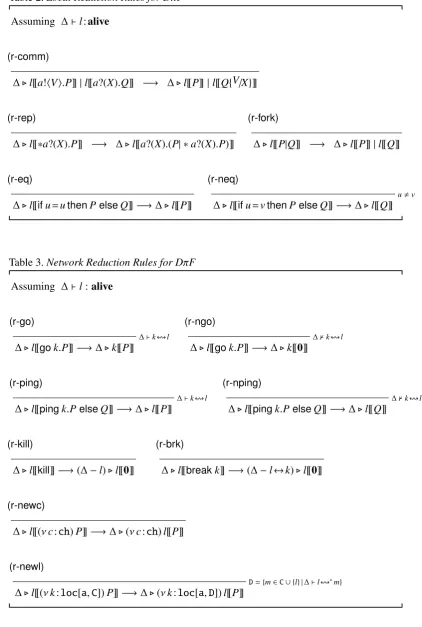
alive; this is the intent of the predicate ∆ ` l : alive. Table 2 gives the standard rules for local communication, and the management of replication, matching and parallelism, derived from the corresponding rules for Dπin [20]. The communica-tion rule(r-comm)depends on a standard notion ofsubstitution Q{V/X}, the details of which we omit. Intuitively the valueV is matched against the pattern X, and the resulting substitution is applied to Q. Of course ifV does not match X a runtime error occurs, but these could be eliminated by the use of a simple, and standard, type system.

The rules in Table 3 are more interesting. Rules(r-go) and(r-ngo)state that a mi-gration is successful depending on the accessibility of the destination; mimi-gration is asynchronous in the sense that code at the source location still migrates, irrespec-tive of the destination’s accessibility. Similarly,(r-ping) and(r-nping)are subject to the same condition for the respective branchings; they however have a more syn-chronous flavour to them since the branching outcome is visible at the testing loca-tion. Ping may also be seen as a form of perfect failure detector [5]; note however that l[[ping k.P elseQ]] yieldspartial information about the state of the underly-ing network. More precisely, it can only determine thatk is inaccessible, but does not give information on whether this is caused by the failure of node k, the ab-sence of the linkl↔k, or both; see Example 4. The rules (r-kill),(r-brk)make the obvious changes to the current network. Finally(r-newc)and(r-newl)regulates the generation of new names. We consciously choose not to express name generation as a (reversible) structural rule since, in practice, this would require some form of resource acquisition and initialisation which may not be reversible; for similar rea-sons(r-fork) is not structural since we interpret it as thread spawning. But perhaps a stronger justification for our design choice is given by (r-newl), describing the launching of new location. In this case, location creation cannot be reversed and recreated because creation depends on the current state of the network which may change during computation. More specifically, inl[[(νk:loc[a,C])P]] the location

l requeststo generate a new (live) locationk, with connections to the locations men-tioned in C. But the ability to establish these connections depends on the existing connectivity of the the parent location l. There are a number of reasonable possi-bilities as to what to do in this situation: we felt it was most realistic to establish a connection from the new locationkto the parentl, and in addition, to only establish connections to those locations inCwhich areaccessiblefrom the parentlvia a se-quence of live links; see Example 5. Note also that we do not have a reduction rule for launching new dead locations; one can easily be added, but there is no reason why any such new locations should ever be generated.

Table 2.Local Reduction Rules for DπF

Assuming ∆`l:alive

(r-comm)

∆.l[[a!hVi.P]]|l[[a?(X).Q]] −→ ∆.l[[P]]|l[[Q{V/X}]]

(r-rep)

∆.l[[∗a?(X).P]] −→ ∆.l[[a?(X).(P| ∗a?(X).P)]]

(r-fork)

∆.l[[P|Q]] −→ ∆.l[[P]]|l[[Q]]

(r-eq)

∆.l[[ifu=uthenPelseQ]]−→∆.l[[P]]

(r-neq)

∆.l[[ifu=vthenPelseQ]]−→∆.l[[Q]] u,v

Table 3.Network Reduction Rules for DπF

Assuming ∆`l:alive

(r-go)

∆.l[[gok.P]]−→∆.k[[P]]

∆`k!l

(r-ngo)

∆.l[[gok.P]]−→∆.k[[0]]

∆0k!l

(r-ping)

∆.l[[pingk.PelseQ]]−→∆.l[[P]]

∆`k!l

(r-nping)

∆.l[[pingk.PelseQ]]−→∆.l[[Q]]

∆0k!l

(r-kill)

∆.l[[kill]]−→(∆−l).l[[0]]

(r-brk)

∆.l[[breakk]]−→(∆−l↔k).l[[0]]

(r-newc)

∆.l[[(νc:ch)P]]−→∆.(νc:ch)l[[P]]

(r-newl)

∆.l[[(νk:loc[a,C])P]]−→∆.(νk:loc[a,D])l[[P]]

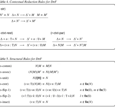
Table 4.Contextual Reduction Rules for DπF

(r-str)

N0 ≡N ∆.N−→∆0_{.M M ≡M}0

∆.N0 −→∆0.M0

(r-ctxt-rest)

∆ +n:T.N −→ ∆0+n:U.M ∆.(νn:T)N −→ ∆0.(νn:U)M

(r-ctxt-par)

∆.N −→ ∆0.N0 ∆.N|M −→ ∆0.N0|M

Table 5.Structural Rules for DπF

(s-comm) N|M ≡ M|N

(s-assoc) (N|M)|M0 ≡ N|(M|M0)

(s-unit) N|l[[0]] ≡ N

(s-extr) (νn:T)(N|M) ≡ N|(νn:T)M n<fn(N)

(s-flip-1) (νn:T)(νm:U)N ≡ (νm:U)(νn:T)N n_<fn(U), m_<fn(T)

(s-flip-2) (νl:T)(νk:U)N ≡ (νk:U−l)(νl:T+k)N l∈fn(U)

(s-inact) (νn:T)N ≡ N n_<fn(N)

T−landT+lhave the obvious definitions:

T−l =

      

T ifT= ch

loc[S,C\ {l}] ifT= loc[S,C] T+l =       

T ifT= ch

loc[S,C∪ {l}] ifT= loc[S,C]

The rules(r-ctxt-par)and(r-ctxt-rest)allow reductions to occur under contexts; note that the latter is somewhat non-standard, but as reductions may induce faults in the network, it may be that the status and connectivity of the scoped (location) namen

is affected by the reduction, thereby changingTtoU. Also in the former it is worth remarking, that since the reduction semantics is only defined on configurations, the free names ofMare guaranteed to occur in∆.

Example 4 (Syntax and Reductions) Let ∆ represent the network h{l,a};{hl,li}i

consisting of a channel a and a live node l and M1the system

(νk2:loc[a,∅]) (νk1:loc[d,{l,k2}]) (l[[a!hk2i.P]]|k2[[Q]])

Here M1 has two new locations k1, k2, where k1 is dead and linked to the existing

node l and k2is alive linked to k1. Although∆only contains one node l, the located

process l[[a!hk2i.P]] (as well as k2[[Q]]) is running on a network of three nodes,

two of which, k1, k2 are scoped, that is not available to other systems. We can

informally represent this implicit network by

d - t - d

l k1 k2

where the nodes◦and•denote live and dead nodes respectively. Note that the same network could be denoted by the system N1

(νk1:loc[d,{l}]) (νk2:loc[a,{k1}]) (l[[a!hk2i.P]]|k2[[Q]])

Note also that the two systems are structurally equivalent, M1 ≡ N1, through (s-flip-2). As a notational abbreviation, in future examples we will omit the status annotationa in live location declarations and simply denote location types of the formloc[a,C]asC; so for example system N1would be given as

(νk1:loc[d,{l}]) (νk2:{k1}) (l[[a!hk2i.P]]|k2[[Q]])

If O is an observer defined as

l[[a?(x).pingx.ok!hielseNok!hi]]

then the configuration∆.N1|O can reduce in two steps to

∆.N1|O−→ · −→(νk1:loc[d,{l}]) (νk2:{k1}) (l[[P]]|k2[[Q]]|l[[Nok!hi]])

The rules(r-comm),(r-str)and(s-extr)are used for the first reduction involving com-munication and subsequent scope extrusion of k2on channel a at l, and(r-nping)for

the second reduction involving the ping test by the observer on the newly discovered location k2; when describing derivation of reductions we generally do not mention

the use of contextual rules of Table 4.

This example highlights the fact that even though the observer has taken the nega-tive branch when pinging k2, it can only deduce that k2is unreachable from the host

location, l; it cannot infer anything else about location k2 in terms of its status, its

connections to other locations, and the code residing there, k2[[Q]].

Example 5 Consider the systemlaunchNewLocdefined by

l3[[a!hl1i]]|l3[[a?(x).(νk:{x,l2,l4,l5})P]]

running on a network∆consisting of five locations l1, . . . ,l5, all of which are alive

except l4, with l2 connected to l1 and l3, and l3 connected to l4. Diagrammatically

this is easily represented as:

d d t

d d

-

A A

A U A A A K

l1

l2 _l

3 l4

l5

Formally describing∆is slightly more tedious:

• ∆N is{a, l1, l2, l3, l4, l5}

• ∆L is given by{hl1,l1i, hl2,l2i, hl3,l3i, hl5,l5i | {z }

live locations

, hl1,l2i, hl2,l3i, hl3,l4i | {z }

live links

}.

When we apply the reduction semantics to the configuration ∆. launchNewLoc, the rule(r-comm)is used first to allow the communication of the value l1 along a,

that is

∆.launchNewLoc −→ ∆.l3[[(νk:{l1,l2,l4,l5})P{l1/x}]]

We highlight that the communication instantiates the variable x in the type of k to l1.

At this point(r-newl)can be used to launch the declaration of k to the system level. However, when launched, k turns out to be connected only to{l1,l2,l3}because: • the location from where the new location k is launched, that is l3, is automatically

connected to k

• l1and l2are reachable from the location where k is launched, namely l3; we have ∆` l3!∗l1 and∆` l3!∗l2.

• l4 and l5are not accessible from l3; l4 is dead and thus it is not accessible from

any other node; l5on the other hand, is completely disconnected.

So the resulting configuration is:

∆.(νk :{l1,l2,l3}) l3[[P{l1/x}]]

The network∆of course does not change, but if we focus on the system l3[[P{l1/x}]],

d d t

d d d

-

A A

A U A A A K

Q Q

Q Q s Q

Q Q Q k

l1

l2 _{l3 l}

4

l5

k

Reduction Barbed Congruence: We borrow the framework of [18] to define a variant of a contextual equivalence, originally proposed in [22], to be able to compare the behaviour of arbitrary systemsMandNrunning on the same network ∆, denoted as:

∆|= M N (3)

We first require some preliminary definitions.

Definition 6 (Typed Relation) Atyped relationover systems is a family of binary relations between systems, R, indexed by network representations. We write ∆ |=

M R N to mean that systems M and N are related byRat index∆, that is M R_∆ N, and moreover∆. M and∆.N are valid configurations.

The definition of our equivalence hinges on what it means for a typed relation to be

contextual, which must of course take into account the presence of the network.

First let us define what kinds of observing systems are allowed to run on a given net-work. The intuition of avalidobserver systemOin a distributed setting∆, denoted as∆`O O, is thatOoriginates from some live location,freshto the observed

system, migrates to any location in loc(∆N) to interact with (observe) processes there and then returns back to the originating fresh location  to compare its

observations with other observers. Our formal definition will not actually mention this fresh home location, as we leave it to the observer itself to both generate

and manage it. But a major consequence of this view of observers is that, in view of the reduction rule (r-ngo), observing code can never reach dead locations; this constraint is reflected in the following formal definition of∆`_O O.

Definition 7 (Observers) ∆`_O O is the least relation which satisfies:

• ∆`<sub>O</sub>l[[P]] if fn(P)⊆∆N and∆`l:alive • ∆`<sub>O</sub>(νn:T)N if (∆ +n:T)`_O N

• ∆`O M|N if ∆`O M and∆`O N

Definition 8 (Contextual typed relations) A typed relationRover configurations iscontextualif:

(Parallel Systems)

• ∆|= MR N and∆`O O implies ∆|= M|OR N|O and∆|=O|MRO|N

(Network Extensions)

• ∆|= MR N and n fresh to ∆ implies ∆+n:T|= MR N

Definition 9 (Reduction barbed congruence) First we define the adaptation of the other standard relations required to definereduction barbed congruence.

Barb Preserving: ∆.N ⇓a@ldenotes anobservable barbexhibited by the

configu-ration∆.N, on channel a at location l. Formally, it means that∆.N −→∗ ∆0.N0 for some∆0. N0such that N0 ≡ M|l[[a!hVi.Q]]and∆ ` l:alive. Then, we say a typed relationRover configurations isbarb preservingwhenever∆|= N R M and∆.N ⇓a@limplies∆.M ⇓a@l.

Reduction Closed: A typed relationRover configurations isreduction closed when-ever∆ |= N R M and∆.N −→ ∆0._N0 _implies∆. _{M −→}∗ ∆0 ._M0 _{for some} ∆0_.

M0 such that∆0 |=N0 R M0.

Then, calledreduction barbed congruence, is the largest symmetric typed relation

over configurations which is:

• barb preserving

• reduction closed

• contextual.

We leave the reader to check that for each index∆the relation∆is an equivalence

relation.

As expected, in a setting with both node and link failures one can discriminate more than in a setting with node failures only. In particular, we were unable to encode a synchronous move in our calculus, even in the presence of thepingconstruct which offers perfect failure detection; we discuss this in the following example.

[16]. Assuming∆` l:alive, the behaviour of this construct could be defined as

(r-move)

∆.l[[movek.PelseQ]]−→∆.k[[P]]

∆`k!l

(r-nmove)

∆.l[[movek.PelseQ]]−→∆.l[[Q]]

∆0k!l

It would be tempting to implement themoveconstruct in our language, considering l[[mvk.PelseQ]]as a macro for

l                    

(νa,b)          

gok.(b?().P|gol.a?().gok.b!hi)

|a!hi |monitorak.Q

                             

where a,b < fn(P,Q). In essence, our implementation sends P to k as an input

guarded process on the scoped channel b, goes back to the source location, l, to signal the successful arrival of P at k, by synchronising on the scoped channel a, and finally goes back to k to release P by outputting on b. This implementation uses mutual exclusion on the scoped channel a, together with the macromonitora k.Q.

This macro repeatedly tests the accessibility of a location k from the hosting loca-tion l and launches Q locally at l when k becomes inaccessible. Before it performs every accessibility test, monitora k.Q synchronizes on the channel a; this ensures

that either k[[P]]or l[[Q]](but not both) is eventually released, as required. The mon-itor process, derived from [10,14], which we denote bymonitorak.Q is encoded in

our language as:

(νtest:ch)(test!hi | ∗test?().a?().pingk.(test!hi |a!hi)elseQ)

Assuming∆l,k = h{l,k},{hl,li,hk,ki,hl,ki}i, the construct l[[move k.P elseQ]]and

its corresponding implementation l[[mvk.P elseQ]] turn out to be observational equivalent in a framework whereonly location failureis allowed.

This is howevernot truein our setting, where link failures may also occur, because from the contextuality property ofwe can conclude

∆l,k |=l[[movek.PelseQ]]|l[[breakk]] 6 l[[mvk.PelseQ]]|l[[breakk]] (4)

More specifically, on the right hand side of (4) we can reduce to a state where b?().P reaches k successfully whilegol.a?().gok.b!hialso manages to go back to l as well, and subsequently synchronises on channel a successfully, thereby blocking monitorak.Q. Now if at this point, the link l↔k breaks because l[[breakk]]reduces,

branches P and Q are blocked. This state can never be reached by the configuration

∆l,k.l[[movek.PelseQ]]|l[[breakk]]on the left hand side, where branching is an

atomic operation2_.

Example 11 (Distributed Servers) Let∆represent the following network:

d d d 1 ) P P P P P i P P P P P q l k2 k1

Formally∆is determined by letting∆N be{l,k1,k2,req,ret}and∆Lbe {hl,li, hk1,k1i, hk2,k2i, hl,k1i, hl,k2i, hk1,k2i}.

The distributed server implementations,servDand srvD2Rt, presented earlier in the Introduction, Section 1, are no longer reduction barbed congruent relative to∆, as in this extended setting, the behaviour of systems is also examined in the context of faulty links. It is sufficient to consider the possible barbs in the context of a client such as l[[req!hl,reti]]and a fault inducing context which breaks the link l↔k1.

C₃ = [−]|l[[req!hl,reti]]|l[[breakk1]]

Stated otherwise, if the link l ↔ k1 breaks, srv2Rt will still be able to operate

normally and perform a barb on ret@l; servD, on the other hand, may reach a state where it blocks since migrating back and forth from l to k1becomes prohibited

and as a result, it would not be able to emit a barb ret@l. However consider the alternative remote serversrvMtr, defined as:

(νdata)                                          l                                  

req?(x,y).(νsync)                 

gok1.data!hx,synci

|monitork1.gok2.gok1.data!hx,synci |sync?(x).y!hxi

                                                  

|k1                    

data?(x,y).          

gol.y!hf(x)i

|monitorl.gok2.gol.y!hf(x)i                                                                       

using a simplified version of the monitor macro of Example 10 which does not synchronise on the channel a for every test. It is defined as

monitork.Q⇐(νtest:ch)(test!hi | ∗test?().pingk.test!hielseQ)

In order to establish∆|=srv2RtsrvMntr directly from the definition of reduction barbed congruence, we would need to compare the behaviour of the two systems relative to all valid contexts. But in the next section we will develop more realistic methods for establishing such identities.

In the next example we examine the interplay between dead nodes and dead links and their respective observation. This example exposes some of the complications we shall encounter when we develop a bisimulation theory for our language.

Example 12 (Network Observations) Let∆l be the simple network with one live location l, denoted and depicted as:

∆l = h{l,a},{hl,li}i = dd

and consider the following three networks,

∆1 = ∆l+k:loc[d,{l}] = d - t

l k

∆2 = ∆l+k:loc[d,∅] = d t

l k

∆3 = ∆l+k:loc[a,∅] = d d

l k

These are the implicit networks for the system l[[a!hki]]in the three configurations

∆l.Ni, where Ni are abbreviations for

N1 ⇐ (νk:loc[d,{l}])l[[a!hki]]

N2 ⇐ (νk :loc[d,∅])l[[a!hki]]

N3 ⇐ (νk :loc[a,∅])l[[a!hki]]

3 A partial view labelled transition system for DπF

It would be tempting to define a bisimulation equivalence based on actions of the form

∆.M −→µ ∆0. M0

Here we argue that this would not be adequate, at least if the target is to characterise reduction barbed congruence.

Example 13 (Partial Views) Let∆lbe the network in which there is only one node l which is alive, defined earlier in Example 12, and consider the system M1defined

by

(νk1:{l}) (νk2:{k1}) (νk3:{k1,k2})l[[a!hk2,k3i.P]]|k2[[Q]]

Note that when M1 is running on∆l, due to the new locations declared, the code

l[[a!hk2,k3i.P]]is effectively running on the followingimplicitnetwork:

d d

d d

*

H H_Hj H H H Y

6

?

l k1

k3

k2

(5)

Let us now see to what knowledge of this implicit network can be gained by an observer O at site l, such as l[[a?(x,y).O(x,y)]], where O(x,y)is a process with free variables x and y. Note that prior to any interaction, O is running on the network

∆l, and thus, is only aware of the unique location l. By inputting along a, it can gain knowledge of the two names k2 and k3, thereby evolving to l[[O(k2,k3)]]. Yet,

even though it is in possession of these two names, it cannot discover their status in terms of liveness of the nodes and links between them and other free locations, such as k2 ↔k3, nor can it interact with code residing at any of these locations,

such as k2[[Q]]. This is due to the fact that the observer is not aware of the local

name k1 and thus cannot determine a path to k2 and k3and discover the full extent

of the sub-network with nodes l, k2and k3, which can be denoted diagrammatically

as

d

d d

6

?

l

k3

Rather, the observer’s view of the sub-network with nodes l, k2 and k3 looks more

like

d _{? ?}

l k2 k3

This means that there is now a difference between the actual network being used by the system, (5), and the observer’sviewof that network; the observer has apartial viewof the network. However, the formalism of our current network does not allow us to represent the differing observer partial view of the network.

A closer inspection of the above example reveals that our requirements for multiple network views are even more complicated. For instance, the network status infor-mation relating to the newly discovered nodes k2and k3are not necessarily hidden

forever from the observer and may become accessible later through subsequent interactions. For example, if P and O(k2,k3)stand for

b!hk1i.P0 and b?(x).gox.gok2.pingk3.R1 elseR2

respectively, the observer can interact on channel b with P, gain the knowledge of the scoped location k1, determine the live path l!k1 ! k2 and subsequently

discover information such as the liveness of k2and k3and the live link k2!k3. An lts semantics has to record the differences between the network and the ob-servers view of networks. A new network representation for our specific case there-fore needs first and there-foremost, distinguish between observable nodes and unobserv-able ones such as k2 and k3, but also to keep network status (that is liveness and connections) relating to the unobservable nodes k2 and k3 that may later become observable. This requires extra information being recorded in network representa-tions.

Definition 14 (Effective LinkSet) A linkset L is effective if it satisfies the

condi-tion:

L₀l:alive implies _@k.L `l↔k

Effective linkset do not represent links where one of the endpoints is dead since these turn out to be unobservable by the constructs of DπF. The operation

|L| = L \ {hl,ki,hk,li | L₀ l:alive}

converts any linkset into an effective linkset by removing links with dead endpoints. For any set of namesN ⊆Nwe also define the filtering effective linkset

oper-ation

Definition 15 (Effective network representations) Aneffective network represen-tationΣis a triplehN,O,H i, where:

• N is a set of names, as before, divided intoloc(N)andchan(N)

• Ois aneffective linkset, denoting the live locations and links between them that areobservableby the context

• His anothereffective linkset, denoting the live locations and links between them that arehidden(or unreachable) to the context.

The only consistency requirements are that:

(1) dom(O)⊆loc(N); the observable live state concerns locations inN

(2) dom(H)⊆loc(N); the hidden live state concerns locations inN

(3) dom(O)∩dom(H)=∅; live state cannot be both observable and hidden.

Effective network representations embody the notion ofobserver partial view dis-cusses above. The intuition is that an observer running on a network representation Σknows about all the names inΣN and has access to all the locations indom(O); as a result, it knows the state of every location indom(O) and the live links between these locations. The observer, however, does not have access to the live locations indom(H). As a result, it cannot determine the live links between them nor can it distinguish them from dead nodes. Dead nodes are not represented directly inΣ, but they can be easily seen to beloc(N)\dom(O ∪ H); that is, all the location names inN that are not mentioned in eitherOorH. We will refer to them as the deadset ΣD . We also note that the effective network representation Σ does not represent live links where either end point is a dead node, since these can never be used nor observed. Summarising,Σholds all the necessary information from the observer’s point of view, that is, the names known,N, the known state, O, and the state that can potentially become known in future, as a result of scope extrusion,H.

As before, we use notation such asΣN, ΣO andΣH to access the fields of Σ and note that any network representation∆can be translated into an effective network representationΣ(∆) in the obvious manner:

• the set of names remains unchanged,Σ(∆)N = ∆N

• the accessible state and connections,Σ(∆)O, is simply|∆L|

• the hidden state,Σ(∆)H, is simply the empty set∅, since∆does not encode any live locations inaccessible to the observer.

There is also an obvious operation for reducing an effective network representation Σinto a standard one,∆(Σ):

We note two properties about the operation∆(Σ); firstly, it does not represent any links to and between dead nodes in ∆(Σ)L; secondly, it not longer distinguishes between accessible and inaccessible states. Whenever we wish to forget about such distinctions inΣ, we can transformΣinto theΣ(∆(Σ)); this we abbreviate to↑(Σ). For a discussion on how effective network representations allow us to accommodate the observers view, as discussed in Example 13, see Example 21 below.

We need to generalise the notation developed on page 7 for standard network rep-resentations∆to these effective representationsΣ; these were judgements relating to the system view of the network. In addition, sinceΣalso describes the observer partial-view, we define similar notation for this restricted view, and denote such judgements by `_O. Extracting information from effective networks is straightfor-ward:

Definition 16 (System/Partial-View Information Extraction from Effective Networks)

• Σ` l:alivewhenever∆(Σ)` l:alive.

• Σ` l↔k whenever∆(Σ)` l↔k

• Σ` l!k ifΣ `l↔k andΣ`l,k:alive.

• Σ`<sub>O</sub>l:alivewheneverΣO `l:alive • Σ`Ol↔k wheneverΣO `l↔k

• Σ`_OO whenever

            

O= l[[P]] andΣ`_O l:alive, fn(P)⊆ ΣN

O= (νn:T)M andfn(T)⊆dom(ΣO), Σ +n:T`O M

O= M|N andΣ`<sub>O</sub> M, Σ`_O N

It is worth pointing out that Σ ` l ↔ k if and only if Σ ` k _!l, because Σ is an effective linkset and thus only records links between live locations, as stated earlier in Definition 14. Definition 16 also extends Definition 7 (valid observers) to effective networks, denoted as Σ `<sub>O</sub> O: even though valid observers may still use any known name in ΣN as before, they can now only be located at accessible locations, that isΣ `_O l:alive, and define new locations that are only connected to accessible locations, that isfn(T)⊆dom(ΣO), so as to respect the partial view.

We can not rely on∆(Σ) in order to define how the effective network representation Σ is updated. This has to be done directly; modifying the liveness conditions is straightforward:

• Σ−l=hΣN, ΣO \ {hl,ki,hk,li |k∈dom(ΣO)}, ΣL\ {hl,ki,hk,li |k∈dom(ΣH)}i • Σ−l↔k= hΣN, ΣO\ {hl,ki, hk,li}, ΣH \ {hl,ki, hk,li}i

arises if there is someki which is observable, that is indom(ΣO), and some otherkj indom(ΣH). In this case any unobservable links involvingkj, or accessible fromkj, now become observable, via the newly observable link betweenkiandl, and thence via the link fromltokj.

It will be convenient to first define a function which returns the set of new links which have to be added to the observable component of Σ when a fresh name is added.

Definition 17 (Link types) If Σ is an effective network representation, and n is fresh toΣ, letlnkO(n:T,Σ)be defined by the following two clauses:

• lnkO(l:loc[a,C],Σ)=       

{hl,ki |k ∈C} ∪ {hl,li} ∪S

k∈C[k]ΣH ifC∩dom(ΣO), ∅

∅ ifC∩dom(ΣO)= ∅

• lnkO(n:T,Σ)=∅, otherwise

In most cases this is actually empty, but in all cases it returns a linkset which is a

component, as defined on page 6; that is a linkset in which all nodes are mutually accessible.

With this function we can now define how to augment an effective network repre-sentation. In the following definitions we assumeaandlarefreshtoΣ:

• Σ +a:ch = hΣN∪ {a}, ΣO, ΣHi • Σ +l:loc[d,C] = hΣN ∪ {l}, ΣO, ΣHi

• Σ +l:loc[a,C] =       

hΣN ∪ {l}, ΣO, H1i ifC∩dom(ΣO)= ∅ hΣN ∪ {l}, O2, H2i ifC∩dom(ΣO)_, ∅ whereH₁= ΣH ∪ {hl,ki |k ∈C} ∪ {hl,li}

O₂= ΣO∪lnkO(l:loc[a,C],Σ) H₂= ΣH \lnkO(l:loc[a,C],Σ)

Here the fresh live locationlis added to eitherΣO orΣH depending on its links. If it is not linked to any observable location, C∩dom(ΣO) = ∅, then the new fresh location is not reachable from the context and is therefore added to ΣH. If, on the other hand, it is linked to an observable location,C∩dom(ΣO),∅, then it becomes observable as well. Moreover, in this case we have to make observable all previ-ously hidden links now made accessible by the fact thatl becomes observable, as we have explained above; these links,lnkO(l: loc[a,C],Σ), have to be transferred fromΣH toΣO. The following example elucidates this operation for extending ef-fective networks.

net-workΣ, with six locations l,k1, . . . ,k5:

Σ = *

N

z }| { {l,k1,k2,k3,k4,k5},

O z}|{ {hl,li},

{hk1,k1i,hk2,k2i,hk3,k3i,hk1,k2i,hk2,k3i,hk4,k4i} | {z }

H

+

According to Definition 15, l is the only observable location by the context; lo-cations k1, . . . ,k4 are alive but not reachable from any observable location while

the remaining location, k5, is dead since it is not indom(ΣO∪ΣH). Moreover, the

linkset representing the hidden state,ΣH, can be partitioned into two components, K₁ = {hk1,k1i,hk2,k2i,hk3,k3i,hk1,k2i,hk2,k3i} and K2 = {hk4,k4i} whereas the

linkset representing the observable state,ΣO, consists of one component,{hl,li}.

The operation Σ + k0:loc[a,{l}] makes the fresh location, k0, observable in the

resulting effective network, since it is linked to (thus reachable from) the observable location l. The operations Σ + k0: loc[a,∅] and Σ +k0 :loc[a,{k1}] both make

k0 hidden in the resulting network because in both cases k0 is not linked to any

observable nodes: in Σ +k0:loc[a,∅] k0 is completely disconnected whereas in Σ +k0:loc[a,{k1}]k0 is only linked to the hidden node k1.

Finally, the operationΣ+k0:loc[a,{l,k1}]affects bothΣOandΣH. This means that

k0 itself becomes observable, since it is linked to l; but as a side effect, the hidden

components reachable through it, that is[k1]L =K1, becomes observable as well;

herelnkO(k0 :loc[a,{l,k1}],Σ)consists of{hk0,li, hk0,k1i} ∪ {k0,k0} ∪ K1.

Thus, according to the above definition, this updated network translates to:

Σ +k0:loc[a,{l,k1}] = hΣN∪ {k0}, ΣO∪({hk0,li, hk0,k1i})∪ K1, ΣH \ K1i

= *

N

z }| { {l,k1,k2,k3,k4,k5,k0},

{hl,li,hk1,k1i,hk2,k2i,hk3,k3i,hk0,k0i,hl,k0i,hk0,k1i,hk1,k2i,hk2,k3i} | {z }

O

,{hk4,k4i} | {z }

H +

Definition 19 (Effective Configuration) A system M subject to an effective net-workΣis said to be an effective configurations ifffn(M)⊆ ΣN.

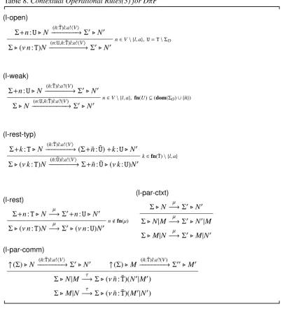
Table 6.Operational Rules(1) for DπF

Assuming Σ`l:alive

(l-out)

Σ.l[[a!hVi.P]]−l−−−−:a!hV→i Σ.l[[P]]

Σ`Ol:alive

(l-fork)

Σ.l[[P|Q]] −→τ Σ.l[[P]]|l[[Q]]

(l-in)

Σ.l[[a?(X).P]]−−−−−→l:a?(V) Σ.l[[P{V/X}]]

Σ`Ol:alive, V⊆ΣN

(l-in-rep)

Σ.l[[∗a?(X).P]]−→τ Σ.l[[a?(X).(P| ∗a?(X).P)]]

(l-eq)

Σ.l[[ifu=uthenPelseQ]]−→τ Σ.l[[P]]

(l-neq)

Σ.l[[ifu=vthenPelseQ]]−→τ Σ.l[[Q]] u,v

Our lts for DπF will be defined in terms of judgements over effective configurations which take the form

Σ.M −→µ Σ0. M0 (6)

whereµcan be an internal action,τ, an input action, (˜n : ˜T)l :a?(V) or an output, (˜n : ˜T)l : a!hVi, adopted from [19,18]; we also have the novel labels, kill : l and

l=k, denoting external location killing and link breaking respectively.

Table 7.Network Operational Rules(2) for DπF

Assuming Σ`l:alive

(l-kill)

Σ.l[[kill]]−→τ (Σ−l).l[[0]]

(l-brk)

Σ.l[[breakk]]−→τ Σ−(l↔k).l[[0]]

(l-halt)

Σ.N−kill:−−→l (Σ−l).N

Σ`Ol:alive

(l-disc)

Σ.N−→l=k Σ−(l↔k).N

Σ`Ol↔k,l,k

(l-go)

Σ.l[[gok.P]]−→τ Σ.k[[P]]

Σ`k!l

(l-ping)

Σ.l[[pingk.PelseQ]]−→τ Σ.l[[P]]

Σ`k!l

(l-ngo)

Σ.l[[gok.P]]−→τ Σ.k[[0]]

Σ0k!l

(l-nping)

Σ.l[[pingk.PelseQ]]−→τ Σ.l[[Q]]

Σ0k!l

(l-newc)

Σ.l[[(νc:ch)P]]−→τ Σ.(νc:ch)l[[P]]

(l-newl)

Σ.l[[(νk:loc[a,C])P]]−→τ Σ.(νk:loc[a,D])l[[P]]

D={m∈C∪ {l} |Σ`l!∗_m}

The more challenging rules are found in Table 8: they are adaptations of the stan-dard rules for actions-in-context from [19], extended to deal with the interaction be-tween scoped location names and their occurrence in location types. For instance, the rule(l-open) filters the type of scope extruded locations by removing links to locations that are already dead and that will not affect the effective networkΣ; this is done through the operationT\ΣD defined as expected:

ch\ {l1, . . . ,ln}= ch loc[S,C]\ {l1, . . . ,ln}=loc[S,C\ {l1, . . . ,ln}] Recall that ΣD is the set of dead locations in Σ. A side condition is added to

Table 8.Contextual Operational Rules(3) for DπF

(l-open)

Σ+n:U.N−−−−−−−−→(˜n: ˜T)l:a!hVi Σ0.N0 Σ.(νn:T)N−−−−−−−−−−−→(n:U,˜n: ˜T)l:a!hVi Σ0.N0

n∈V\ {l,a},U=T\ΣD

(l-weak)

Σ+n:U.N −−−−−−−−→(˜n: ˜T)l:a?(V) Σ0.N0 Σ.N −−−−−−−−−−−→(n:U,˜n: ˜T)l:a?(V) Σ0.N0

n∈V\ {l,a},fn(U)⊆(dom(ΣO)∪ {n}˜)

(l-rest-typ)

Σ+k:T.N−−−−−−−−→(˜n: ˜T)l:a!hVi (Σ+n˜: ˜U)+k:U.N0 Σ.(νk:T)N −−−−−−−−→(˜n: ˜U)l:a!hVi Σ+n˜: ˜U.(νk:U)N0

k∈fn( ˜T)\ {l,a}

(l-rest)

Σ+n:T.N−→µ Σ0+n:U.N0 Σ.(νn:T)N−→µ Σ0.(νn:U)N0

n_<fn(µ)

(l-par-ctxt)

Σ.N−→µ Σ0.N0 Σ.N|M−→µ Σ0.N0|M Σ.M|N−→µ Σ0.M|N0

(l-par-comm)

↑(Σ).N−−−−−−−−→(˜n: ˜T)l:a!hVi Σ0.N0 ↑(Σ).M−−−−−−−−→(˜n: ˜T)l:a?(V) Σ00.M0 Σ.N|M−→τ Σ.(νn˜: ˜T)(N0|M0)

Σ.M|N−→τ Σ.(νn˜: ˜T)(M0|N0)

The internal communication rule (l-par-comm)also contains subtleties: communi-cation is defined in terms of the system view (↑(Σ)) rather than the observer view dictated by Σ; the intuition is that internal communication can still occur, even at locations that the observer cannot access. Thus the premises are defined in terms of the ability to output and input of systems with respect to the maximal observer view, ↑(Σ). The rules(l-rest)and(l-par-ctxt)should be relatively straightforward. Finally,

(l-rest-typ) is a completely novel rule which filter any links exported in location types when the other endpoint of the link is still scoped. For brevity, the premise of this rule exploits the fact that the networkΣ +k1:loc[S1,C1]+k2 :loc[S2,C2] can be also expressed asΣ +k2 : loc[S2,C2\ {k1}]+k1 : loc[S1,C1∪ {k2}] whenever

Example 20 (Scope Extruding Network Information) Consider the extended net-workΣwhere l and k1are accessible by the context, that isΣ`Ol:alive, k1 :alive.

For the effective configurationΣ.(νk2:{k1})l[[a!hk2i]]we can derive the transition Σ.(νk2:{k1})l[[a!hk2i]]

(k2:{k1})l:a!hk2i

−−−−−−−−−−→Σ +k2 :{k1}.l[[0]]

using (l-out) and (l-open). The transition label denotes the scope extrusion of the fresh location k2 with the information that it is connected to k1. We can also have

the sequence of transitions

Σ.(νk2:{k1})l[[a!hk2i]] kill:k1

−−−→

Σ−k1.(νk2:{k1})l[[a!hk2i]]

(k2:∅)l:a!hk2i

−−−−−−−−→

(Σ−k1)+k2:∅.(νk2:{k1})l[[a!hk2i]]

whereby the context first kills k1before performing the input on a at l. The second

transition is still derived using(l-out)and(l-open)but, this time ,the side-condition

U = T\ΣD of(l-open)ensures that we scope extrude k2 with different information,

stating that it is completely disconnected, thus inaccessible (hidden). This transi-tion captures the fact that even though the link between k2 and k1 still exists, this

information cannot be discovered and used by the context to access k2. In fact, k2

is added toΣOin the resulting configuration of the first case of scope extrusion but

added to(Σ−k1)H in the second case.

Example 21 Let us revisit Example 13 to see the effect of the observer O on M1;

this observer runs on the effective networkΣl having only one location l which is alive, that isΣ(∆l). This effectively means calculating the result of M1 performing

an output on a at l.

If we consider a sub-derivation where k1 is not restricted, then an application of (l-out)and(l-par-ctxt), followed by two applications of(l-open)gives

Σl +k1:{l}. M01 α

−→Σl+k1:{l}+k2:{k1}+k3:{k1,k2}.l[[P]]|k2[[Q]] (7)

where M₁0 is(νk2:{k1})(νk3:{k1,k2})l[[a!hk2,k3i.P]]|k2[[Q]]andαis the action(k2: {k1},k3:{k1,k2})l:a!hk2,k3i.Note that(l-rest)can not be applied to this judgement,

since k1occurs free in the actionα. However (7) can be re-arranged to read

Σl +k1:{l}. M01 α

−→Σl+k2:∅+k3:{k2}+k1:{l,k2,k3}.l[[P]]|k2[[Q]]

moving the addition of location k1 in the reduct to the outmost position. At this

point,(l-rest-typ)can be applied, to give

Σl .M1 β

where β is the action (k2 : ∅, k3 : {k2})l : a!hk2,k3i; that is β is filtered of any

occurrence of k1in its bound types.

Note that the residual network representation,Σl+k2 :∅+k3 :{k2}describes

partial-view network, with a hidden part that is not available to the observer. Eliding any channel names, the network evaluates to

h{l,k2,k3}, {hl,li}, {hk2,k2i,hk3,k3i,hk2,k3i}i

where the liveness of k2 and k2 and the connection between them is hidden. This

effective network may be represented diagrammatically as:

d d d 6 ? l k3 k2

where the links of hidden components are denoted with dashed lines.

With these actions we can now define in the standard manner a bisimulation equiv-alence between configurations, which can be used as the basis for contextual rea-soning. Let us write

Σ|= M≈wrong N

to mean that there is a (weak) bisimulation between the configurationsΣ. M and Σ.Nusing the current lts actions. This new framework can be used to establish pos-itive results. For example, forΣl,k = h{a,l,k},{hl,li,hk,ki,hl,ki},∅i, one can prove

Σl,k |=l[[pingk.a!hielse0]]≈wrongk[[gol.a!hi]]

by giving the relationRdefined as:

R=                                                         

hΣl,k.M , Σl,k .Ni | hM,Ni ∈ Rsys

hΣl,k−l. M , Σl,k−l.Ni | hM,Ni ∈ R1sys hΣl,k−k.M , Σl,k−k.Ni | hM,Ni ∈ R2sys hΣl,k−l↔k.M , Σl,k−l↔k.Ni | hM,Ni ∈ R3sys hΣl,k−l,l↔k. M , Σl,k−l,l↔k.Ni | hM,Ni ∈ R3sys hΣl,k−k,l↔k.M , Σl,k−k,l↔k.Ni | hM,Ni ∈ R3sys hΣl,k−l,k. M , Σl,k−l,k.Ni | hM,Ni ∈ R3sys hΣl,k−l,k,l↔k. M , Σl,k−l,k,l↔k.Ni | hM,Ni ∈ R3sys

where

Rsys =                 

hl[[pingk.a!hielse0]] , k[[gol.a!hi]]i

hl[[a!hi]] , l[[a!hi]]i

hl[[0]] , l[[0]]i

                

R1

sys = Rsys ∪ {hl[[pingk.a!hielse0]], l[[0]]i} R2

sys = Rsys ∪ {hl[[0]], k[[gol.a!hi]]i} R3

sys = Rsys ∪

hl[[0]], k[[gol.a!hi]]i, hl[[pingk.a!hielse0]], l[[0]]i

However we can argue, at least informally, that this notion of equivalence is too discriminating and the labels too intentional, because it distinguishes between sys-tems running on a network, where the differences in behaviour are impossible to observe. Problems arise because the current labels contain information relating to thehidden partof an effective network, which is not observable by valid contexts.

Example 22 Let us consider a slight variation on the system M1 used in

Exam-ple 13 and ExamExam-ple 21:

M2⇐(νk1 :{l})(νk2:{k1})(νk3 :{k1})l[[a!hk2,k3i.P]]|k2[[R]]

again running on the (effective) networkΣl = h{l,a},{hl,li},∅i. Note that the code l[[a!hk2,k3i.P]]|k2[[R]]is now effectively running on the following implicit network,

d d

d d

*

H H_Hj H H H Y

l k1

k3

k2

a slight variation on that for M1. It turns out that Σl |= M1 6≈wrong M2

This is not because k2[[Q]]in M1and k2[[R]]in M2 may be different - the condition Σ `_O l : alive in (l-out) and (l-in) of Table 6 prohibits input or output labels at hidden locations - but rather because the configurations give rise todifferentoutput actions, on a at l. The difference lies in the types at which the locations k2 and k3

are exported; as we have seen, inΣl .M1 the output label isβ = (k2:∅, k3:{k2})l:

there is a difference in the type associated to the scope extruded location k3; in the

first label, the scope extruded k3 is linked to the newly scope extruded k2 whereas

in the second label it is not.

However if k1 does not occur in P, (for example if P is the trivial process0) then

k1 can never be scope extruded to the observer and thus k2 and k3 will remain

inaccessible in both systems. This means that the presence (or absence) of the link k2↔k3can never be checked and thus

Σl |= M1 M2

The extra label information relating to the hidden part of the network is also indis-tinguishable from information relating to dead nodes, as is shown in the following example.

Example 23 Let us reconsider the three configurationsΣl.Ni for i= 1,2,3from

Example 12 whereΣl = Σ(∆l)= h{l,a},{hl,li},∅i. We have already argued that these three configurations should not be distinguished. However, our lts specifies that all three configurations perform the output with different scope extrusion labels, namely:

Σl.N1

(k:loc[d,{l}])l:a!hki

−−−−−−−−−−−−−→ h{l,k},{hl,li},∅i.l[[0]]

Σl.N2

(k:loc[d,∅])l:a!hki

−−−−−−−−−−−−→ h{l,k},{hl,li},∅i.l[[0]]

Σl.N3

(k:loc[a,∅])l:a!hki

−−−−−−−−−−−−→ h{l,k},{hl,li},{hk,ki}i.l[[0]]

More specifically,

• Σl . N1’s transition label states that the scope extruded location k is dead and

linked to l

• Σl . N2’s label states that the scope extruded location k is deadand completely

disconnected

• whereas Σl . N3’s label states that k is alive but completely disconnected, and

thus added to the hidden part ofΣl.

With these labels, the three configurations will be distinguished by the bisimulation equivalence≈wrongwhereas, according towe have

Σl |= N1 N2 N3

since no observer would be able to distinguish the difference in the state of k.

4 A bisimulation equivalence for DπF

We first outline the revision to our labelled transitions. Currently, the actions of these transitions use types of the form T = ch or loc[S,{k1, . . .kn}], where the latter indicates the liveness of a location and the nodes ki to which it is directly linked. We change these to new types of the form

L,K= {hl1,k1i, . . . ,hli,kii}

whereL,Kare components. Intuitively, these represent the new live nodes and links, which are made accessible to observers by the extrusion of a new location. Alterna-tively, this is the information which is added to the observable part of the network representation, ΣO, as a result of the action. This means that our labels now de-scribe information at the level ofaccessibility pathsbetween locations as opposed to direct connections only. We have already developed the necessary technology to define these new types, in Definition 17.

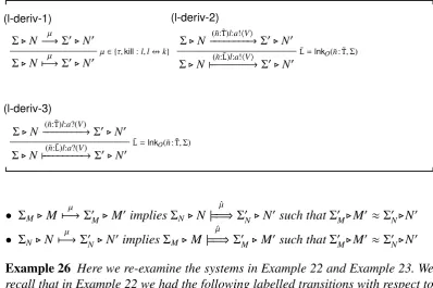
Definition 24 (A (derived) labelled transition system for DπF) This consists of a collection of transitionsΣ.N 7−→µ Σ0._N0_{, where}µ_{takes one of the forms:}

• (internal action) -τ

• (bounded input) -(˜n: ˜L)l:a?(V) • (bounded output) -(˜n: ˜L)l:a!hVi • (external location kill) -kill:l

• (external link break) - l=k

The transitions in the derived lts for DπF are defined in Table 9. The rules (l-deriv-2) and (l-deriv-3) transform the types of bound names using the function lnkO(˜n:

˜

T,Σ); this is simply a version of the function defined in Definition 17 to deal with sequences of type declarations:

lnkO((n,n˜) : (T,T˜),Σ) = lnkO(n:T,Σ),lnkO(˜n: ˜T,(Σ +n:T))

These revised transitions give rise to a new(weak) bisimulation equivalenceover configurations,≈, defined in the usual way, but based onderived actions. Our

defi-nition uses the standard notation for weak actions, namely µ

|==⇒denotes

_τ

7−→∗

_µ

−→

_τ

7−→ ∗

, and b µ

|==⇒denotes

• 7−→τ ∗

ifµ=τ

• µ

|==⇒otherwise.

Table 9.The derived lts for DπF

(l-deriv-1)

Σ.N−→µ Σ0.N0 Σ.N7−→µ Σ0.N0

µ∈ {τ,kill:l,l=k}

(l-deriv-2)

Σ.N −−−−−−−−→(˜n: ˜T)l:a!hVi Σ0.N0 Σ.N `−−−−−−−−→(˜n: ˜L)l:a!hVi Σ0.N0

˜

L=lnkO(˜n: ˜T,Σ)

(l-deriv-3)

Σ.N−−−−−−−−→(˜n: ˜T)l:a?(V) Σ0.N0 Σ.N`−−−−−−−−→(˜n: ˜L)l:a?(V) Σ0.N0

˜

L=lnkO(˜n: ˜T,Σ)

• ΣM.M µ 7−→Σ0

M. M 0

impliesΣN.N ˆ µ |==⇒Σ0

N.N 0

such thatΣ0_M.M0 ≈Σ0 N.N

0

• ΣN.N 7−→µ Σ0_N.N0 impliesΣM.M

ˆ µ

|==⇒Σ0_M.M0such thatΣ0_M.M0 ≈Σ0_N.N0

Example 26 Here we re-examine the systems in Example 22 and Example 23. We recall that in Example 22 we had the following labelled transitions with respect to the original lts:

Σl.M1 µ1

−→Σ +k2:∅+k3:{k2}.(νk1:{l,k2,k3})l[[P]]|k2[[Q]] Σl.M2

µ2

−→Σ +k2:∅+k3:∅.(νk1:{l,k2,k3})l[[P]]|k2[[R]]

ButΣlcontains only one accessible node l; extending it with the new node k2, linked

to nothing does not increase the set of accessible nodes. Further increasing it with a new node k3, linked to the inaccessible k2(in the case ofΣ.M1) also leads to no

increase in the accessible nodes. Correspondingly, the calculations oflnkO(k2:∅,Σ)

andlnkO(k3:{k2},(Σ +k2:∅))both lead to the empty link set.

Formally, we get the derived action

Σ. M1 α

7−→ Σ +k2:∅+k3:{k2}.(νk1:{l,k2,k3})l[[P]]|k2[[Q]]

where αis(k2:∅, k3:∅)l : a!hk2,k3i. Similar calculations gives exactly the same

derived action from M2: Σ. M2

α

7−→ Σ +k2:∅+k3:∅.(νk1:{l,k2,k3})l[[P]]|k2[[R]]

Furthermore, if P contains no occurrence of k1, we can go on to show Σ+k2:∅+k3:{k2}.(νk1:{l,k2,k3})l[[P]]|k2[[Q]]≈

Since k1cannot ever be scope extruded to the observer, we are guaranteed that the

state of k2 and k3 together with the code located at these locations, that is k2[[Q]]

and k2[[R]], are forever inaccessible to the observer. This means that we can match

anyτ-move by k2[[Q]] on the left hand side by the empty move (and viceversa for

k2[[R]]) and any move by l[[P]]on either side by that same identical move.

On the other hand, if P is a!hk1i, the subsequent transitions are different: ((Σ +k2 :∅)+k3 :{k2}).(νk1:{l,k2,k3})l[[P]]|k2[[Q]]

α1

7−→ . . .

((Σ +k2 :∅)+k3 :∅).(νk1 :{l,k2,k3})l[[P]]|k2[[R]] α2

7−→ . . .

where

α1 is (k1:{k1↔k2,k1↔k3,k2↔k3})l:a!hk1i α2 is (k1:{k1↔k2,k1↔k3})l:a!hk1i

We note that the link type associated with β1 includes the additional component {hk2,k3i}, that was previously hidden, but is now made accessible as a result of

scope extruding k1;β2on the other hand, does not have this information in its link

type. Based on this discrepancy betweenα1andα2we have Σl.M1 6≈Σl.M2

In addition, if M1 and M2 were running on the same network, say (5), and k2[[Q]]

and k2[[R]] were different systems, this could be verified after the scope extrusion

of k1: scope extruding k1would make k2observable, enabling(l-out)and(l-in)to be

applied to the code Q and R running at k2.

Example 27 Revisiting Example 23, the three different actions ofΣl .N1, Σl .N2

andΣl . N3 now abstract to the same action Σl .Ni α

7−→ . . . .l[[0]]for i = 1,2,3

whereαis the label(k:∅)l:a!hki. Thus we have

Σl.Ni ≈Σl.Nj where i, j=1,2,3

as required.

5 Full-Abstraction

Σ(∆). We next redefine reduction barbed congruence for effective configurations. The reduction relation over effective configurations

Σ.M −→Σ0. M0

is simply obtained by reusing the rules defined earlier in Tables 2, 3, 4 and 5, substitutingΣfor∆3_{. Note that all the side-conditions used in these rules can also} be applied toΣusing the notation developed on page 21.

We refine the notion of a barb for effective configurations, intuitively restricting them to observable locations, that is those inΣO.

Definition 28 Σ.N ⇓a@ldenotes anobservable barbexhibited by the configuration Σ.N, on channel a at location l. Formally, it means thatΣ.N −→∗Σ0.N0for some

Σ0_.

N0 such that N0≡ (νn˜: ˜T)M|l[[a!hVi.Q]]where l,a<n and l˜ ∈dom(Σ0O).

We also extend the definition of contextual relations to effective configurations. The novel aspect of this extended definition is that we now relate configurations with arbitrary effective networks, as long as their observable part, that is ΣN and ΣO, coincide. Because of this, valid observers, that isΣ`_OO, valid network extensions, that isfn(T)∈dom(ΣO), and name freshness, that isn_<ΣN, in the definition below need only be defined with respect to one effective network.

Definition 29 (Contextual relations over effective configurations) A relation R

over effective configurations iscontextualif:

(Observable Network equality)

• Σ. MRΣ0.N implies ΣN = Σ0_N andΣO = Σ0_O

(Parallel Systems)

• Σ. MRΣ0_.

N andΣ`_OO implies − Σ.M|ORΣ

0_.

N|O

− Σ.O|MRΣ0_.

O|N

(Network Extensions)

• Σ. MRΣ 0_.

N and

fn(T)⊆dom(ΣO), n_<ΣN

implies Σ +n:T. MRΣ0+n:T.N

With these modifications, we extend Definition 9 forreduction barbed congruence

for effective configurations, denoted as

ΣM .M ΣN.N

and defined as the largest relation over effective configurations that isbarb preserv-ing,reduction closedandcontextual.

Note that this enables us to compare arbitrary configurations,ΣM.MandΣN.N, but it can be specialised to simply comparing systems running on the same network. Let us write

Σ|= M N

to mean thatΣ. M Σ.N. Then, for example, the notation (3) used in Section 2 can be taken to mean

Σ(∆)|= M N

where the effective networkΣ(∆) has no hidden state.

At this point, we are in a position to state the main result of the paper:

Theorem 30 Suppose Σ.M, Σ0.N are effective configurations in DπF such that

ΣN = Σ0

N andΣO = Σ 0 O. Then

Σ.M Σ0.N if and only if Σ.M ≈Σ0.N

This general result can also be specialised to the notation for comparing systems relative to a given network:

Corollary 31 In DπF,Σ |= N M if and only ifΣ|= N ≈ M.

The proof of the general theorem, which is quite complex, is detailed in the fol-lowing two sections. The first section outlines the proof forsoundness, that is, the adequacy of the derived action bisimulation as a means to show that two configu-rations are reduction barbed congruent:

Σ1.M1 ≈Σ2.M2 implies Σ1.M1 Σ2.M2

The second section outlines the proof forcompleteness, that is, for any two config-urations that are reduction barbed congruent, we can give a derived action bisimu-lation to show this:

Σ1.M1 Σ2.M2 implies Σ1.M1≈ Σ2.M2

this turns out to be in accordance with our definition of reduction barbed congru-ence. This assumption also suffices to guarantee that when two configurations are bisimilar, their observable network is equivalent (see Proposition 33).

5.1 Soundness

The main task in proving that derived action bisimulation is sound is showing that ≈is contextual.

One aspect worth highlighting about any two bisimilar configurationsΣ.M, Σ0.N

in≈is that the observable parts of the respective effective networksΣandΣ0, that is ΣN,Σ0

N and ΣO, Σ 0

O, coincide (up to our symmetric interpretation of links, that is l↔k is the same as k↔l); we show this in Proposition 33. This allows us to smoothly apply the Definition 29, Contextuality, which also requires configurations to have the same observable network. Intuitively, if they did not, one configuration could transition with a label whose form depends on the observable part of the network, such askill : korl = k forΣO andl : a?(V) forΣN, that the other could not (weakly) match. For this purpose, we find it convenient to

• denote the observable pairhN,Oiin an effective configuration asI. • refer to the observable part of an effective networkΣasI(Σ).

We start by proving our earlier claim that the observable networks of bisimilar con-figurations coincide. This proposition uses a lemma stating that there is a special relationship between derivedsilent actions and residual networks: internal transi-tions do not change the state of the network, unless akillor abreaklprocess in the configuration itself is consumed.

Lemma 32 IfΣ.N 7−→τ Σ0._N0 _thenΣ0 _{is either:}

(1) Σ (2) Σ−l (3) Σ−l↔k

PROOF. A straightforward induction on the inference ofΣ.N 7−→τ Σ0._N0_.

Proposition 33 (Bisimulation and Observable Networks)

IfΣM. M≈ ΣN.N thenI(ΣM)=I(ΣN).

PROOF. We already assume thatΣM N = Σ

N

N; we just need to show thatΣ M O = Σ

N O. Assumehl,ki ∈ΣM

O. SinceΣ M