PROCESSING SPECTRORADIOMETRY DATA FOR THE SIMULATION OF SOIL PHYSICOCHEMICAL
PARAMETERS
José M. Filippini Alba
1*, Lucia E. C. Cruz
2, Jorge R. Ducati
3, Henrique N. da Cunha
4and João M. M. Domingues
51D.Sc. (Geoscience), Researcher, Environmental Planning Laboratory, Embrapa Clima Temperado, Pelotas-RS-Brazil
2D.Sc. (Agronomy), Autonomous, Pelotas-RS-Brazil
3D.Sc. (Physical), Professor/Researcher, State Research Center for Remote Sensing and Meteorology, Federal University of
Rio Grande do Sul State, Porto Alegre – RS – Brazil
4Degree in Geography, M.Sc. (Remote Sensing), Federal University of Rio Grande do Sul State
5Geological Engeniar, Federal University of Pelotas, Pelotas-RS-Brazil
ARTICLE INFO ABSTRACT
In spite of its restricted use, due to data quantity and difficulty of interpretation, spectroradiometry is a potential application for precision agriculture. In this study, samples of lowland soils were collected according to a regular grid. Each sample was analyzed by conventional physicochemical methods (Al, Ca, K, Mg, Na, P and clay) and spectroradiometry (2151 bands, 350 to 2500 nm).The work aimed to simulate physicochemical variables using data from spectroradiometry bands. Dependence analysis, Factor analysis and Cluster analysis were applied gradually until the determination coefficients (R2) of the regression models reach100%. That occurred when at least two of the three statistical methods were applied. Two different strategies were highlighted: (1) Factor analysis with high number of factors extracted; (2) Factor Analysis with a few factors followed by cluster analysis for population segregation. Although option (1) was simpler, option (2) allowed outliers discard, in the way that the geostatistical maps were improved.
Copyright © 2019, José M. Filippini Alba et al. This is an open access article distributed under the Creative Commons Attribution License, which permits unrestricted use, distribution, and reproduction in any medium, provided the original work is properly cited.
INTRODUCTION
Reflectance Spectroradiometry (KARDEVÁN, 2007) is a nondestructive low cost method for analysis of minerals, soils, rocks, vegetation and water, with short time of process and calibration dependency. Measurements can be take neither on field or in laboratory, whenever the same principles of remote sensing imagery caption are used (LIEW, 2001). Hence, agricultural, biological, geological and mineralogical studies can be performed. According to Liaghat & Balansundram (2010), “Precision Agriculture (PA) is changing the way people farm, since it offers a myriad of potential benefits in profitability, productivity, sustainability, crop quality, environmental protection, on-farm life quality, food safety and rural economic development. PA is an innovative, integrated
*Corresponding author: José M. Filippini Alba,
D.Sc. (Geoscience), Researcher, Environmental Planning Laboratory, Embrapa Clima Temperado, Pelotas-RS-Brazil
and internationally standardized approach aiming to increase the efficiency of resource use and to reduce the uncertainty of decisions required to manage variability on farms. PA has been hailed as one of the most scientific and modern approaches to production agriculture in the 21st century, as it epitomizes a better balance between reliance on traditional knowledge and information and management-intensive technologies”. Acknowledging a more specific perspective regarding geo processing and remote sensing, GE et al. (2011) mentioned that: “Over the past few decades, agricultural production has progressed from the machinery age to the information age and has been growing use of the term (PA), which implies small-scale information-based optimization of inputs for overall gains in profitability and environmental stewardship. Geo-spatial technologies, including geographic information systems, the global positioning system and remote sensing, are extensively utilized in PA. Presently, PA has been deployed in almost all aspects of agriculture production. As an
ISSN: 2230-9926
International Journal of Development Research
Vol. 09, Issue, 08, pp. 28875-28880, August, 2019
Article History:
Received 22nd May, 2019
Received in revised form 03rd June, 2019
Accepted 11th July, 2019
Published online 28th August, 2019
Available online at http://www.journalijdr.com
Key Words:
Databases, Big data, Spectroradiometry, Pedology
Citation: José M. Filippini Alba, Lucia E. C. Cruz, Jorge R. Ducati et al.2019. “Processing spectroradiometry data for the simulation of soil physicochemical parameters”, International Journal of Development Research, 09, (08), 28875-28880.
information- and computation-intensive technology, the success of PA depends strongly upon highly efficient and reliable methods for site-specific field information gathering and processing”. Therefore, an interaction between PA and spectroradiometry appears as a line of research for future developments. Lee et al. (2003) worked with 270 superficial samples of Alfisol, Entisol and Ultisol. The explained variance for the simulated models of pH, Ca, Mg and P from spectroradiometry data was more than 79% on calibration stage. However, these percentages were less than 50% for K and organic matter (OM). Selige et al. (2006) analyzed the relation between OM and N contents and percentage of clay and sand in a topsoil using hiperspectral aerial data. The R2 of the adjusted models was equal to 0.9, 0.92, 0.71 and 0.95, respectively. Ge et al. (2011) revised the topic “remote sensing of soil properties in precision agriculture”. They considered 15 parameters roughly, including major elements, physical variables, texture, Na and Zn; the prevailing method was reflectance spectroradiometry in Vis-IR interval with measurements in laboratory and different statistical multivariate methods. According to the authors, “Apparently the biggest obstacle for commercial soil sensor development is inconsistency of models obtained from different studies at different locations”. Rossel et al. (2006) made a similar development, but in that case, the use of complex statistical multivariate methods was emphasized as multiple regression, aspect also mentioned for Cohen et al. (2007), and principal components. Mineralogical features of the spectra were highlighted. Values of Al, Ca and P contends, CEC and electrical conductimetry were poorly explained by the simulation models (R2< 0,5). Nocita et al. (2012) indicated that the spectroradiometry reflectance related to the organic carbon level of soils is dependent on the soil moisture content in a nonlinear way. Vendrame et al. (2012) worked with Cerrado Latosols (Brazil), when soil texture and mineralogy were contrasted to NIR spectroradiometry data. The variance explained by simulation models (R2) was lesser or equal 60% for silt and fine sand percentage, hematite and goethite content. Most of the authors suggests spectroradiometry as a potential procedure for PA. However, variability of data, due to the occurrences of different groups of samples, and the complexity of multivariate statistical data process, can affect interpretation. Cluster analysis was never mentioned. Thus, this work aims to discuss the usage of multivariate statistical methods, including procedures of sample segregation, so that some parameters of the soil can be simulated with spectroradiometry data in Southern Brazilian lowlands.
MATERIAL AND METHODS
The area of interest is located in latitude 31° 49’ 12.34” S and longitude 52° 27’ 57.78” W, in the experimental station “Terras Baixas” of “Embrapa Clima Temperado”, municipality of Capão do Leão, Rio Grande do Sul State, Brazil. Within a Pedology perspective, a Haplic Planosol (Brazilian System of Soil Science) derived from Quaternary sandy sediments covers the area. The A horizon is moderate, with clayey – sandy texture, plane relief with low local altitude (10 m) and bad drainage, land use alternates crops and pastures in 3years x 2years regime, usually. Climate is Humid Subtropical (CFa), according to Köppen classification (apud WREGE et al., 2012, p. 322) – the coldest month averaging 0 °C, at least one month averaging above 22 °C and at least four months averaging 10 °C. No significant precipitation difference between seasons, neither dry month in summer. A
geor referenced regular grid of soil samples was performed before October/2012 with 15 m sampling pass, according to 7 transects of 7 samples each, totaling 49 samples (density of about 60 samples/ha) . A Sokkia SET 610 total station and a Sokkia GSR 2600 GPS receiver were used. The soil layers 0 – 0.1 m and 0.1 – 0.2 m were collected by means of a cutting shovel in each point of the regular grid. Therefore, the materials were stocked in plastic bags using field notebook and paper labels for registration. After that, samples were dried in air, lumps were crumbled and the fraction smaller than 2 mm was sieved. Chemical analysis were performed in the Vegetal Nutrition Laboratory of Embrapa Clima Temperado (Pelotas-RS-Brazil) for Al, Ca, K, Mg, P and organic matter (OM) content and granulometric composition (sand, silt and clay). Spectroradiometry measurements were made in collaboration with the State Research Center for Remote Sensing and Meteorology of the Federal University of Rio Grande do Sul (Porto Alegre-RS-Brazil) in 2013. Reflectance of soil samples was determined with the FieldSpec3 equipment, considering wavelength between 350 nm and 2500 nm and spectral resolution of 1 nm. Original spectral data were transformed to relative reflectance. Statistical methods were applied by the Statistical Package for Social Sciences, SPSS® and the respective interpolated maps were developed in two parts: (1) semivariograms through software GS+®; (2) Krigging through the Geographic Information System ArcGIS®.
RESULTS AND DISCUSSION
Statistical description of datasets: All variables showed moderate variance according to the coefficients of variation (Table 1). On the other hand, the spectra of the soil samples were very similar to each other (Figure 1). Physicochemical variables presented moderate to low Pearson correlation values between them, sometimes with negative values. For instance, Al-Ca = -0.518, Al-K = -0.447, Al-OM = 0.412, clay-OM = 0.407, clay-Al = 0.398, K-P = 0.365 e K-Na = 0.335. Correlation coefficients between the physicochemical variables and the reflectance bands were almost constant when wavelength reached 750 nm. Al, Ca, clay and P presented negative near zero values, K was near 0.36, Mg was near -0.6, Na was near 0.14 and OM was near -0.15. However, correlation coefficients between the reflective bands were very significant, oscillating within the interval of 0.80 to 0.99. Therefore, both sets of data have low variance and correlations were low between physicochemical variables each other or between physicochemical variables and reflective bands.
Table 1. Basic
Variable Al, cmolc.L-1
Clay, % Ca, cmolc.L-1
K, cmolc.L-1
OM, % Mg, cmolc.L-1
Na, mg.dm-3
P, mg.dm-3
[image:3.595.121.472.220.412.2]RB, % (B350 to B2500) CofV = Coefficient of Variation; m –
Figure 1. Vis-IR Reflectance Spectra of each soil sa
Figure 2. Cumulated explained variance for
Table 2. Coefficient of determination (R2
Variable Al, cmolc.L-1
Ca, cmolc.L-1
Clay, % K, cmolc.L-1
Mg, cmolc.L-1
OM, % Na, mg.dm-3
P, mg.dm-3
28877 International Journal of Development Research,
Basic statistics of the variables considered in this study
m - M Mean CofV
0.1 - 1.1 0.8 32%
16 – 25 19.8 12%
1.0 – 2.1 1.8 15%
0.1 – 0.3 0.12 35%
1.5 – 2.8 1.9 18%
0.4 – 1.1 0.7 16%
14 - 42 23 25%
5 - 21 10 40%
0.053 – 0.998 0.08 to 0.8 15 to 18%
– M = minimum – Maximum; MO = Organic matter; ND = Number of determinations; RB = Relative reflectance of VIS-IR bands.
IR Reflectance Spectra of each soil sample. RR = Relative Reflectance
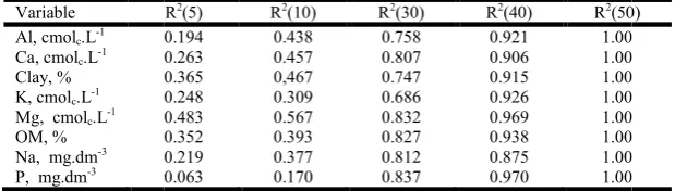
2. Cumulated explained variance for first 50 factors of the reflective bands dataset
2
) of regression models of each variable as a linear function of factors for differ number of extracted factors
R2(5) R2(10) R2(30) R2(40) R2(50)
0.194 0.438 0.758 0.921 1.00
0.263 0.457 0.807 0.906 1.00
0.365 0,467 0.747 0.915 1.00
0.248 0.309 0.686 0.926 1.00
0.483 0.567 0.832 0.969 1.00
0.352 0.393 0.827 0.938 1.00
0.219 0.377 0.812 0.875 1.00
0.063 0.170 0.837 0.970 1.00
International Journal of Development Research, Vol. 09, Issue, 08, pp. 28875-28880, August,
ND 49 49 49 49 49 49 49 49 105399
Maximum; MO = Organic matter; ND = Number of determinations;
mple. RR = Relative Reflectance
reflective bands dataset
) of regression models of each variable as a linear function of factors for different
(50) 1.00 1.00 1.00 1.00 1.00 1.00 1.00 1.00
[image:3.595.155.438.439.620.2] [image:3.595.140.450.681.769.2]Factor Analysis is a multivariate method related to Principal Components, so its success for modeling information was predicted. Thus, when Ge et al. (2011) mentioned “…inconsistency of models obtained from different studies at different locations”, they are suggesting segregation of the sample population. Nocita et al. (2012) and Vendrame (2012) confirmed this idea, for moisture of soil and other pedologic parameters respectively influencing reflective light data. However, population was always cons
by data processing methods, without any segregation.
Table 3. Means of the groups (G1-4) defined by cluster analysis and result of nonparametric tests Kruskal Whitney
Variable Al,cmolc.L-1
Ca,cmolc.L-1
Clay, % K,cmolc.L-1
Mg, cmolc.L-1
OM, % Na, mg.dm-3
P, mg.dm-3
[image:4.595.91.516.214.516.2] [image:4.595.112.494.553.742.2]Samples or groups (KW and MWU)
Figure 3. Line graphic including the means of the groups (G1
Figure 4. Multivariate statistical process applied in this work aschart flow
Factor Analysis is a multivariate method related to Principal Components, so its success for modeling information was (2011) mentioned “…inconsistency of models obtained from different studies at re suggesting segregation of the . (2012) and Vendrame et al. (2012) confirmed this idea, for moisture of soil and other influencing reflective light data. However, population was always considered as a whole by data processing methods, without any segregation.
Studying groups (subpopulations)
the regression models or factor analysis increased according to the number of factors considered. Alongside
and variables the greater variance, so more factors will be needed for explaining 100% of variance. Four groups were defined by Cluster Analysis (Table 3).
showed statistical significant values for, at least, the me one group. Group 1 included two samples only, with different combinations of extreme values for Al, K and Na, thus, they were considered outliers. Group 2 had significant high values of K and Na, and clay intermediate.
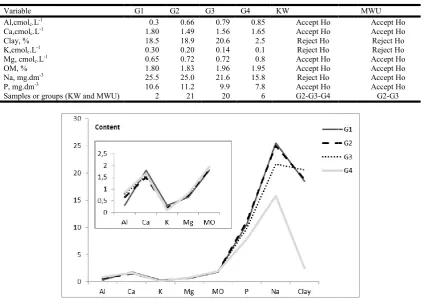
4) defined by cluster analysis and result of nonparametric tests Kruskal Whitney-U (MWU). Ho = no difference among means
G1 G2 G3 G4 KW
0.3 0.66 0.79 0.85 Accept Ho 1.80 1.49 1.56 1.65 Accept Ho 18.5 18.9 20.6 2.5 Reject Ho 0.30 0.20 0.14 0.1 Reject Ho 0.65 0.72 0.72 0.8 Accept Ho 1.80 1.83 1.96 1.95 Accept Ho 25.5 25.0 21.6 15.8 Reject Ho 10.6 11.2 9.9 7.8 Accept Ho
2 21 20 6 G2-G3-G4
Line graphic including the means of the groups (G1-4) defined by Cluster Analysis. First part of the graphic was detailed in the little rectangle
Multivariate statistical process applied in this work aschart flow
Studying groups (subpopulations): The variance explained by the regression models or factor analysis increased according to the number of factors considered. Alongside the more samples and variables the greater variance, so more factors will be needed for explaining 100% of variance. Four groups were defined by Cluster Analysis (Table 3). Clay, K and Na content showed statistical significant values for, at least, the mean of one group. Group 1 included two samples only, with different combinations of extreme values for Al, K and Na, thus, they were considered outliers. Group 2 had significant high values of K and Na, and clay intermediate.
4) defined by cluster analysis and result of nonparametric tests Kruskal-Wallis (KW) and
Mann-MWU Accept Ho Accept Ho Reject Ho Reject Ho Accept Ho Accept Ho Accept Ho Accept Ho G2-G3
4) defined by Cluster Analysis. First part of the graphic
Groups 1 and 2 have a similar behavior (
[image:5.595.106.485.207.790.2]differences are observed for the detailed picture. Group 3 is the richest in clay and Group 4 suggests sandy or silty soil occurrence, due to very low clay content. Regression linear models with 40 factors as independent variables were developed for the physicochemical variables of the groups 2, 3 and 4. Total variance was explained at full and the relation between the dependence variable and the simulated variable was always perfectible linear as it happened with the regression models with 50 factors and all samples.
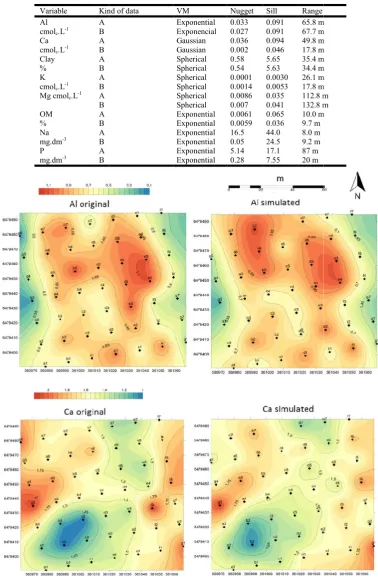
Table 4. Parameters of variograms for original data and simulated data considering 40 factors (G2, G3 and G4). Two samples (o were discarded in the last case: 49 samples and 47 samples were used, respectively. VM = Variogram model. Kind of
Variable Kind of data Al
cmolc.L-1
A B Ca
cmolc.L-1
A B Clay
%
A B K
cmolc.L-1
A B Mg cmolc.L-1 A
B OM
%
A B Na
mg.dm-3
A B P
mg.dm-3 A B
Figure 5. Maps of Al and Ca (cmolc
28879 International Journal of Development Research,
Groups 1 and 2 have a similar behavior (Figure 3), but differences are observed for the detailed picture. Group 3 is the sandy or silty soil very low clay content. Regression linear models with 40 factors as independent variables were developed for the physicochemical variables of the groups 2, 3 and 4. Total variance was explained at full and the relation between the dependence variable and the simulated variable was always perfectible linear as it happened with the regression models with 50 factors and all samples.
The number of factors considered
was equal to the degree of freedom for each group, 6 samples to 5 factors; 20 samples to 19 factors and go on. The statistical process was synthetized in Figure 4.
Spatial analysis: Although data could be simulated by two different methods, both incorporating
one including cluster analysis, the second option is a more embracing method, which can be applied in a greater number of situations.
Table 4. Parameters of variograms for original data and simulated data considering 40 factors (G2, G3 and G4). Two samples (o were discarded in the last case: 49 samples and 47 samples were used, respectively. VM = Variogram model. Kind of
B = Simulated, 40 factors
Kind of data VM Nugget Sill Range Exponential 0.033 0.091 65.8 m Exponencial 0.027 0.091 67.7 m Gaussian 0.036 0.094 49.8 m Gaussian 0.002 0.046 17.8 m Spherical 0.58 5.65 35.4 m Spherical 0.54 5.63 34.4 m Spherical 0.0001 0.0030 26.1 m Spherical 0.0014 0.0053 17.8 m Spherical 0.0086 0.035 112.8 m Spherical 0.007 0.041 132.8 m Exponential 0.0061 0.065 10.0 m Exponential 0.0059 0.036 9.7 m Exponential 16.5 44.0 8.0 m Exponential 0.05 24.5 9.2 m Exponential 5.14 17.1 87 m Exponential 0.28 7.55 20 m
c.L -1
) interpoled by krigging in the lowland station (“Estação Capão do Leão – RS, southern Brazil
International Journal of Development Research, Vol. 09, Issue, 08, pp. 28875-28880, August,
The number of factors considered for the regression models was equal to the degree of freedom for each group, 6 samples to 5 factors; 20 samples to 19 factors and go on. The statistical process was synthetized in Figure 4.
Although data could be simulated by two nt methods, both incorporating factor analysis, but only one including cluster analysis, the second option is a more embracing method, which can be applied in a greater number
Table 4. Parameters of variograms for original data and simulated data considering 40 factors (G2, G3 and G4). Two samples (outliers) were discarded in the last case: 49 samples and 47 samples were used, respectively. VM = Variogram model. Kind of data: A = original;
65.8 m 67.7 m 49.8 m 17.8 m 35.4 m 34.4 m 26.1 m 17.8 m 112.8 m 132.8 m 10.0 m
krigging in the lowland station (“Estação Terras Baixas”),
So, spatial analysis was considered upon data with 40 factors, considering groups 2, 3 and 4. The outliers (group 1) were discarded, consisting of 4,1 % of total variance. Simulated data considered the regression models for each group, allowing reconstitution of the physicochemical variables. The variograms of Al, clay, Mg and OM were similar when the real data and the simulated data were compared (Table 4). However, Ca, K, Na and P showed significant differences. This consideration could be confusing initially, but it can be elucidated by the outliers influence, with extreme values of K and Na.Ca, K and P were strongly affected including the range values. Some variables related to the previous variograms were interpoled by krigging. The maps of Al original and Al simulated were very analogous (Figure 5), but some local differences are related to samples g6 and c7, which were discarded for the second map. Significant differences occurred for the maps of Ca in the same way of the respective variograms (Table 4).
Final Remarks: Physicochemical soil parameters were simulated by spectroradiometry data of the same samples in plain soils from lowlands in Southern Brazil. Both sets of data showed low variability because coefficients of variation were lesser than 40%. The spectroradiometry data showed strong correlation among sequential bands, but low correlation with physicochemical data. Spectra can be discriminated by multivariate criteria, but a visual interpretation, as suggested with mineralogical composition (Ducart et al., 2006), was not possible. Thus, factor analysis was applied on spectroradiometry data in the way that the regression models have got the full simulation of the physicochemical variables, which can be achieved by the determination coefficients of 100%. This particular event happened when 48 factors were extracted. More than 99% of the total variance was accumulated in the two first factors, but the 46 following factors were necessary anyway. A successful simulation with fewer factors was obtained when cluster analysis was applied. Four groups were defined, characterized by different values of K, Na and clay means. One group was interpreted as outliers (two samples). Interpoled maps by krigging were smoother when outliers were discarded and physicochemical groups were considered. This second method could be used when the influence of moisture (Nocita et al, 2012) or different kind of soils (Vendrame et al., 2012) affect data. Most studies have used laboratory measures at the present, so to reach automation, in situ data and temporally changes must be evaluated.
Acknowledgments
The authors are thankful to Lais R. Silva and Bárbara Cosenza by languages revision. Second author had financial support of CAPES. Other contributors were Silvia B.A. Rolim (UFRGS) and Rosemary Hoff (Embrapa) for FieldSpec measuring and Diego S. Vieira, Jones O. Moraes and Mayara Zanchin for initial processing data.
REFERENCES
COHEN, M.; MYLAVARAPU, R.S.; BOGREKCI, I.; LEE, W.S.; CLARK, M.W. Reflectance spectroscopy for routine soil analysis. Soil Sc. 172: 469 - 485, 2007. DUCART, D.F.; CRÓSTA, A.P.; SOUZA FILHO, C.R.
Alteration mineralogy of the Cerro La Mina epithermal prospect,
GE, Y.; THOMASSON, A.; SUI, R. Remote sensing of soil properties in precision agriculture: A review. Frontier
Earth Science, v. 5 (3), p. 229 – 238, 2011.
JÖRESKOG, K.G.; KLOVAN, J.E.; REYMENT, R.A. Geological Factor Analysis. Amsterdam: Elsevier Pub.
Co., 1976, 178p.
KARDEVÁN, P. Reflectance spectroradiometer – a new tool for environmental mapping. Carpth. J. Earth Environ. Sc.,
2: 29-38, 1997.
LEE, W.S.; SANCHEZ, J.F.; MYLAVARAPU, R.S.; CHOE, J.S. Estimating chemical properties of Florida soils using spectral reflectance. Am. Soc. Agricultural Engenieers
46:1443-1453, 2003.
LIAGHAT, S.; BALASUNDRAM, S.K. A review: the role of remote sensing in precision agriculture, Am. J. Agricultural and Biological Sc., 5: 50-55, 2010.
LIEW, S.C. Principles of Remoter Sensing.Singapure: CRISP, 2001. Available: https://crisp.nus.edu.sg/~research/ tutorial/optical.htm. Access: fev 21, 2019.
NOCITA, M.; STEVENS, A.; NOON, C.; WESEMAEL, B. van. Prediction of soil carbon for different levels of soil moisture using Vis-NIR spectrometry. Geoderma 199: 37-42, 2013.
ROSSEL, R.A.V.; WALVOORT, D.J.J.; McBRATNEY, A.B.; JANIK, L.J.; SKJEMSTAD, J.O. Visible, near infrared, mid infrared or combined diffuse reclectance spectroscopy for simultaneous assessment of various soil properties. Geoderma 1331:59-75, 2006.
SELIGE, T.; BÖHNER, J.; SCHMIDHALTER, U. High resolution topsoil mapping using hyperspectral image field data in multivariate regression modeling. Procedures. Geoderma 136: 235-244, 2006.
VENDRAME, P.R.S.; MARCHÃO, R.L.; BRUNET, D.; BECQUER, T.The potential of NIR spectroscopy to predict soil texture and mineralogy in CerradoLatosols.J. Soil Sc. 63: 743-753, 2012.
WREGE, M. S.; STEINMETZ, S.; REISSER JUNIOR, C.; ALMEIDA, I. R. de. (Ed.). Atlas climático da região Sul do Brasil: Estados do Paraná, Santa Catarina e Rio Grande do Sul. Brasília, DF: Embrapa, 2012. 334 p.