3717
THE EFFECT OF ATTRIBUTE DIVERSITY IN THE
COVARIANCE MATRIX ON THE MAGNITUDE OF THE
RADIUS PARAMETER IN FUZZY SUBTRACTIVE
CLUSTERING
1MARJI, 2SAMINGUN HANDOYO, 3IMAM N. PURWANTO, 4 M. YUYUD ANIZAR 1Department of Informatics Engineering, Universitas Brawijaya Malang, Indonesia
2,4Department of Statistics, Universitas Brawijaya Malang, Indonesia
3Department of Mathematics, Universitas Brawijaya Malang, Indonesia
E-mail: 1[email protected], 2[email protected], 3[email protected],4[email protected]
ABSTRACT
The Fuzzy Subtractive Clustering (Fsc) method is applied in many fields because it is able to produce optimal clusters without requiring initial information of many groups as well as on the k-mean method. Unfortunately, in the Fsc method, there is a radius parameter that has a vital role in generating optimal clusters. The magnitude of this radius parameter is hypothetical to be influenced by the variability of the covariance matrix of the dataset. This study investigates the magnitude of radius parameter that resulted in optimal clusters on three datasets with high variability (dataset1), moderate variability(dataset2), and low variability(dataset3) on covariance matrices. In the clustering process, the squash factor and accept ratio parameters are made in constant, while the radius parameter is the determined variable that leads to the optimal cluster achievement. Clustering results are said to be optimal based on two criteria: each cluster consists of at least 2 members, and the clustering produces the smallest Ctm value. The results of this study recommend that prior to clustering with Fsc, it should be calculated first covariance matrix based on the standardized dataset. If the covariance matrix has a high variability, the radius value used is close to 1, the moderate variability is a radius value of about 0.5, whereas the low variability is used near the 0 radius value.
Keywords: Covariance Matrix, Fuzzy Subtractive Clustering, Optimal Cluster, Radius Parameter, Variability
1. INTRODUCTION
In a database system, an object is expressed as a record that occupies rows of a schema or table. The columns of the table state the attributes that describe the object. The attribute whose value varies is known by the term variable. Let A be a group of objects with attributes or variables attached to them. Based on all attributes or variables that are shared by all objects in A, it is desirable to separate or split A into subgroups A1, A2, ..., Ak. The goal to be achieved in clustering is that all objects in a subgroup are expected to have a high similarity. In the conventional clustering method, the size of the resemblance used is the norm or distance[1],[2]. Therefore, information about the object acting as the center of the group is
absolutely necessary to be used as a reference for calculating distance[3].
3718 quickly produces the optimal cluster. Mustakim[6] uses the eigenvector of the covariance matrix as the cluster center initialization. Nevertheless, the k-mean method is still constrained by the parameter k which influences the cluster center initialization.
Some recent applications of the k-mean method are performed by Jumma, et al[7] which protects sensitive information from data mining clustering results, while Sugiantoro and Kiswanto[8] profiles the contents of emails to determine the pattern of email content that interferes with the client or server. Rabbouch, et al[9] proposed a pattern recognition system that uses clustering algorithms in order to detect, calculate and recognize a number of dynamic objects crossing the highway. From the various applications of the k-mean method, the problem of determining a large number of groups (k) that will result in the optimal clustering is a problem that is not easily solved.
Along with the development of fuzzy logic, emerging fuzzy set-based clustering methods, some of which are Fuzzy c-mean and fuzzy subtractive. Chiu[10] identifies the fuzzy model based on cluster estimation, Tafazoli, et al[11] modeling the dependence of a system, not only on its current state but also in its hysteresis using fuzzy subtractive, while Ghosh, et al[12] using fuzzy clustering for unattended detection changes in remote sensing images. The application of subtractive fuzzy in various fields is performed by Chamzini et al[13] predicting the performance of the road headers, optimizing the transient performance of the automatic generation control by Rouhani et al[14] and Ariadji, et al[15] optimizing the direction and length horizontal wells on the X-oil field. The comparison of the performance of Fsc against other methods was done by Bataineh, et al[16] compares the performance of both Fcm and Fsc methods on some experimental data. In Fcm requires a training algorithm and in Fsc it requires setting the radius parameters done by trial and error so that both methods produce the optimal grouping. The merging of Fsc and SOM methods in two-level clustering was done by Lisangan, et al[17]. The fuzzy subtractive appeal is very high for researchers because this method can generate automatic grouping without requiring the determination of the number of groups at the beginning.
The superiority of Fsc in forming clusters automatically without having to provide the cluster
number input seems to make Fsc an easy-to-implement method. In fact, the input of the magnitude of the radius parameters that have an important role in Fsc is still determined by trial and error, so to produce an optimal cluster must be done several times grouping with different radius parameter values and then the optimal cluster is determined based on certain indicators. This study intends that the Fsc implementation can be applied effectively without having to try some radius values by proposing the identification of the variability of each variable in the dataset to be clustered through the covariance matrix. Researchers assume that variability in the dataset greatly affects the magnitude of the radius that produces the optimal cluster, so that if the dataset variability value is known then the radius value can be determined easily, finally, the Fsc method can be implemented effectively.
Based on the above explanation that the number of clusters (k) in k-mean clustering can be solved by the fuzzy-subtractive method in which this method can form groups automatically. However, in the application the Fsc method requires the parameter of the magnitude of the radius (r) that plays an important role in the optimal Fsc application. In this study focused to investigate the magnitude of radius parameters that can result in grouping of the optimal Fsc method. The proposed method is to explore the covariance matrix of the dataset to be clustered and to test several parameters of the radius that will lead to the optimal clustering that produces a small value Ctm. For the purposes of investigating the effect of the covariance matrix on the magnitude of the radius parameter, there are provided three datasets having high[18], moderate[19], and low[20] of covariance matrix variability.
2. LITERATURE REVIEW
3719 clustering methods namely hierarchical and non-hierarchical clustering. Almost all clustering methods require initial information on the number of clusters to be established. This is not an easy setting for getting an optimal clustering. One method that does not require that information is fuzzy subtractive clustering(Fsc).
2.1 Sample covariance matrix
According to Rencher[2], the variance of random variables is the size of variability whereas the covariance is a value which expresses the variation of the value of a random variable in its associative ratios with other random variables. Covariance is the mean product value of the X1 variable deviation on its mean and the X2 variable deviation at the mean. The random variable is positively related, ie if X1 is greater than the mean, then the X2 value also tends to be greater than the mean, the value of the covariance will be positive. Conversely, the two variables are negatively related, ie if X1 is greater than the mean, then the variable X2 tends to be less than the mean, the value of the covariance will be negative. Consider, both X1 and X2 are random variables had mean and
successively, the covariance between X1 and X2 is
(1) while the value of the variance is the covariance value of the variable itself, ie
or (2)
Assumes of an object or a record observed based on p attributes are , the value of the record on the i-th object is , if as much as n number of samples of the object
observed, it will be obtained the size of its variability called the matrix of variance-covariance sample as follows[3]:
(3)
In S the sample variances of the p variables are on
the main diagonal, and all possible pairwise sample covariance appear off the diagonal. The j-th row
(column) contains the covariance of with the other p − 1 variables. There are three approaches to
obtaining S. The first of these is to simply calculate the individual elements sjk. The sample variance of
the j-th variable, sj j= , is calculated as in (2) and
is calculated using (1).
2.2 Fuzzy Set
At the outset, the concept of the fuzzy set was introduced by Professor Lotfi A. Zadeh in 1965. The concept of fuzzy set comes from a
classical set (crisp) of a strict or absolute nature that has only two membership values, if an object is a member of a set then the object has degree membership one and vice versa if the object is not a member of a set then the object has a degree of membership zero. In the fuzzy set, the degree of membership of an object in a set is not strictly defined. The transition characteristics are described in terms of membership functions that make the fuzzy set flexible in modeling linguistic expressions[10].
2.3 Gaussian Membership Function
A function that gives degrees to an object or record of its existence in a set is called a membership function. The membership function will map each record with a membership degree value that has a value between 0 and 1 (Jang et al, 2000). Some form functions that can be used to represent a fuzzy membership function are the triangle, shoulder, Gaussian, and sigmoid curve shapes[11].
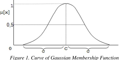
Gaussian membership function is a bell-shaped curve, in which the shape of the membership function is determined by two parameters, namely the center-size or mean (c) and standard deviation (σ). The formula of the Gausian membership function is stated as follows[12]:
[image:3.612.318.522.490.593.2](4) Parameter c determines the location of the center of the curve, and the parameter σ determines the width of the curve of the Gaussian membership function, as in Figure 1 below.
Figure 1. Curve of Gaussian Membership Function
2.4 Fuzzy Subtractive Clustering(Fsc)
3720 greatest distance change on the dendrogram, all possible group members are already formed, while in Fsc, group number will be calculated one by one starting at the beginning of the iteration.
According to Chiu[10], the initial step of clustering with Fsc is to determine the object or record that has the highest potential value to the object around it. Suppose there are n objects or
records potential value of an object can be calculated by the formula:
(5)
Pk is the potential value of k-record, is the k-record, and is the j-record, notation ||.|| is the Euclidean distance, n is the amount of data, is a positive constant known as the radius. An object has a high potential if the object has the largest number of neighbors. After calculating the potential of each object, the object with the highest potential is selected as the center of the group. Suppose is the object selected as the center of the first group, while Pc1 is a measure of the potential of the cluster center in the first group. Furthermore, the potential of the object around it is determined by the formula[10]:
(6)
is the new potential value of object k-th, is a positive constant. This means that objects near the center of the group will experience great potential reductions. The constant causes the object around the center of the group to diminish its potential value. Usually is greater when compared to , ie: = q * where q is squash factor. Once the potential of all objects in a group is reduced, the object with the highest potential is selected as the center of the second group. Furthermore, after obtaining the center of the second group, the potential value of each object is reduced again, and so on.
The center of the group is determined by using two comparative factors namely the accept ratio and reject ratio[11]. Accept ratio is the lower bound of an object that becomes a candidate group center accepted as the center of the group, while the reject ratio is the upper limit of an object that becomes the candidate center group is not accepted as the center of the group. At an iteration, if it is found an object with the highest potential, then
proceed by calculating the potential ratio of the object to the highest potential of an object in the first iteration. There are 3 conditions that may occur in an iteration that is:
a.
If the ratio> accept ratio, then the object is accepted as a new group center.b.
If the reject ratio <ratio≤ accept ratio, then the object is accepted as a new group center if and only if the sum between the ratio and the object's nearest distance to the other existing group center ≥1.c.
If the ratio≤ reject ratio, then no more objects can be considered as a candidate for group center, iteration is stopped[11].According to Chiu[10], the specification of accept ratio = 0.5 and reject ratio = 0.15, whereas the radius is a vector that determines how much influence the cluster center on each variable.
2.5 Cluster Tighness Measure (Ctm)
Optimization of clustering results can be assessed using Ctm, which is formulated with[16]:
(7) M is the number of groups, K is the number of variables, is the standard deviation of the k-th variable in the m-th group, and is the standard deviation of the k-th variable. The value of Ctm is closer to zero, the better of the clusters result obtained.
3. DATA AND METHOD
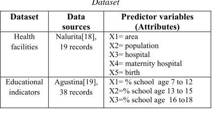
[image:4.612.310.528.624.740.2]The data used in this study are three datasets that have varying covariance matrix variability that is high, moderate, and low respectively[18-20] for dataset1, dataset2, and dataset3. Dataset1 consists of 5 attributes and 19 records, dataset2 consists of 5 attributes and 38 records, while dataset3 consists of 3 attributes and 19 records. The three datasets come from the research data that has been done. Detailed data description can be seen in Table 1.
Table 1. Data Sourcs and Attributes for Three Dataset
Dataset Data
sources Predictor variables (Attributes)
Health facilities
Nalurita[18], 19 records
X1= area X2= population X3= hospital X4= maternity hospital X5= birth
Educational indicators
Agustina[19], 38 records
3721
X4=average in school age 15 X5=literacy minimum age 10 Educational
rate
Yuliantin[20], 19 records
X1= Gross participation rate X2= Net participation rate X3= School participation rate
The method in this research is divided into four stages as follows:
1. Description of data aims to explore the variability contained in the three datasets. The steps in this stage are
a. Normalize the data to equalize the unit of each attribute
b. Calculates the variance of each attribute
c. Calculates covariance between two attributes
d. Draw a boxplot of each attribute e. Assess the variability of each dataset 2. Determining the input parameter values of
the Fsc method other than the radius parameter with a constant [15] ie Accept ratio = 0.5, Reject ratio = 0.15, and Squash factor = 1.25. The amount of radius value used as input is determined by the researcher by considering 2 criteria that each cluster has at least 2 members and small CTM value. In this study is determined using 5 radius values leading to optimal grouping. The first radius value used is 0.5. If clustering is obtained there is still one cluster with only 1 record member then the radius value will be increased, and if the value of CTM obtained is still large enough then the radius value will be decreased. Optimal cluster occurs if the CTM value is small and at least every cluster has 2 members.
3. Clustering with Fuzzy subtractive for each dataset with various radius values using Gaussian membership function, then observation of the clustering results that include:
a. Center each group
b. The degree of membership of each record
c. Members of each group
4. Calculate the Ctm value of each clustering result on each radius parameter
5. Determine optimal clustering results based on criteria:
a. smallest Ctm value, and
b. all the groups that are formed have at least 2 members
4. RESULTS AND DISCUSSION
The data used in this research are 3 datasets which have successively number of variables of for each dataset are 5, 5, and 3 variables. The use of dataset with a different type of variables is intended to determine the effect of the variables type to the number of groups formed by Fuzzy Subtractive. It will also be investigated the effect of variability of each dataset based on the covariance matrix calculated on each dataset after the normalization process (equating the data units).
In the dataset1, the differences in the variability value between one variable to each others variables are quite large. The covariance matrix of dataset1 as follows:
[image:5.612.316.510.466.539.2]The main diagonal of C1 is the variance of each variable, ie: the value=0.80 is the variance of variable X1, 0.087 for variable X2, and so on. Whereas all values that lie outside the main diagonal express the value of covariance ie the value that states the relationship between two variables, for example, ie cov (X1, X3) = cov (X3, X1) = -0.030. On other hand, the Figure 2 present 5 boxplot diagram from each variable of the dataset1.
Figure 2. Boxplot diagram of the dataset1
The bold lines on each box shows the value of mean of each variable. There are not only quite differences in mean value, but also the boxes are devided by mean with not propotional that indicate the distribution of the variables asymmetric.
3722
Figure 3. Boxplot diagram of the dataset2
Generally, the dataset2 has a more symmetrical distribution than dataset1 but has a low intermediate relationship, which is approximately 10% covariance when compared to the covariance of dataset1.
[image:6.612.95.525.63.237.2]The dataset3 has the homogeneous character of both variance and covariance. This is shown in matrix C3 and Figure 4. The value of variance and covariance is almost the same that is 0.06, while the median divides the box into two parts which are relatively proportional
.
Figure 4. Boxplot diagram of the dataset3
Thus, the dataset3 is an example of the symmetrically distributed dataset case and has a homogeneous variance for each variable.
4.2 Clusters Resulted in Fuzzy Subtractive Clustering Method
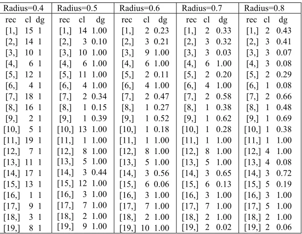
[image:6.612.153.462.477.717.2]Clustering with Fuzzy Subtractive is done with the help of R software. After inputting data on worksheet R, followed by setting input argument parameters ie radius, accept ratio, reject ratio, and squash factor. In this study, the input argument of the radius is set for several different values, while the value of the accept ratio, the reject ratio, and the squash factor is set using only one value. After setting the input parameters, then run the program source code on each dataset to generate the center of the group. This group center will be used as a reference to calculate the degree of membership of each record or object using the Gaussian membership function. A large difference in the value of the radius affects many groups that are formed on each dataset. Table 2 presents the clustering result on dataset1.
Table 2. Clustering Results for the Various Radius Values on Dataset1
Radius=0.4 Radius=0.5 Radius=0.6 Radius=0.7 Radius=0.8 rec cl dg
[1,] 15 1 [2,] 14 1 [3,] 10 1 [4,] 6 1 [5,] 12 1 [6,] 4 1 [7,] 18 1 [8,] 16 1 [9,] 2 1 [10,] 5 1 [11,] 19 1 [12,] 7 1 [13,] 11 1 [14,] 17 1 [15,] 13 1 [16,] 1 1 [17,] 9 1 [18,] 3 1 [19,] 8 1
rec cl dg [1,] 14 1.00 [2,] 3 0.10 [3,] 10 1.00 [4,] 6 1.00 [5,] 11 1.00 [6,] 4 1.00 [7,] 2 0.34 [8,] 1 0.15 [9,] 1 0.39 [10,] 13 1.00 [11,] 1 1.00 [12,] 8 1.00 [13,] 5 1.00 [14,] 3 0.44 [15,] 12 1.00 [16,] 3 1.00 [17,] 7 1.00 [18,] 2 1.00 [19,] 9 1.00
rec cl dg [1,] 2 0.23 [2,] 3 0.21 [3,] 9 1.00 [4,] 6 1.00 [5,] 2 0.11 [6,] 4 1.00 [7,] 2 0.47 [8,] 1 0.27 [9,] 1 0.52 [10,] 1 0.18 [11,] 1 1.00 [12,] 8 1.00 [13,] 5 1.00 [14,] 3 0.56 [15,] 6 0.06 [16,] 3 1.00 [17,] 7 1.00 [18,] 2 1.00 [19,] 10 1.00
rec cl dg [1,] 2 0.33 [2,] 3 0.32 [3,] 3 0.03 [4,] 6 1.00 [5,] 2 0.20 [6,] 4 1.00 [7,] 2 0.58 [8,] 1 0.38 [9,] 1 0.62 [10,] 1 0.28 [11,] 1 1.00 [12,] 8 1.00 [13,] 5 1.00 [14,] 3 0.65 [15,] 6 0.13 [16,] 3 1.00 [17,] 7 1.00 [18,] 2 1.00 [19,] 2 0.02
3723 where,
rec= record number cl=cluster number
dg=degree of membership a record on the cluster
Table 2 presents the output of clustering results from dataset1 with Fsc for radius parameter values between 0.4 and 0.8. The selection of the first radius used as input is r = 0.5 which is then followed by selecting radius value r = 0.4 and r = 0.6. Because the clustering result with radius r = 0.4 obtained as many as 19 clusters which each cluster consisting of only one element, whereas the result of clustering with radius r = 0.6 obtained fewer cluster number that is 14 clusters. Thus to obtain optimal clustering results, then selected radius r = 0.7 and r = 0.8.
In summary, the result of clustering Fsc on dataset1 that is at radius r = 0.4 formed 19 clusters, at r = 0.5 formed 14 clusters which only in clusters 1,2 and 3 respectively have the number of members 3, 2, and 3, while the other cluster consists of only 1 member. In the radius r = 0.6 formed 10 clusters, which there are still 6 clusters consisting of only one member, the cluster 10,9,8,7,5, and 4. Similarly
at radius r = 0.7 formed 8 clusters, and also still found clusters consisting of only 1 member, for example, cluster 7 and cluster 8. While the clustering results on radius r = 0.8 formed 5 clusters which in each cluster at least consists of 2 records.
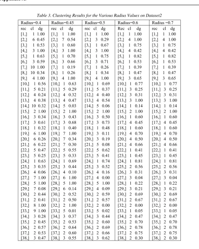
[image:7.612.147.465.429.669.2]The process of selecting the radius parameter values used in clustering dataset2 and dataset3 is almost identical to the selection process of the radius parameter in clustering dataset1. The principal principle is that the first radius parameter value is r = 0.5, followed by r> 0.5 or r <0.5. The clustering results in datasets 2 with radius r = 0.5 formed 5 clusters, whereas in radius r = 0.4 and r = 0.6, 10 clusters and 4 clusters formed respectively. At radius r = 0.4 from 10 clusters formed there are two clusters with one member that is cluster 8 and cluster 9, so no need to continue to try radius value r <0.4. Furthermore, clustering is continued for r = 0.7 which results in 2 clusters which indicate that in the dataset2 the value of the radius parameter is increased close to 1, the clustering of the dataset2 will produce 1 cluster only. Therefore, the next parameter of the radius being tested is r = 0.45. The clustering results of the complete dataset2 and its degree and record number are presented in Table 3 on Appendix A.
Table 4. Clustering Results for the Various Radius Values on Dataset3
Radius=0.07 Radius=0.1 Radius 0.3 Radius=0.5 Radius=0.6 rec cl dg
[1,] 3 1.00 [2,] 2 0.92 [3,] 2 1.00 [4,] 3 0.93 [5,] 1 0.00 [6,] 4 0.84 [7,] 1 0.12 [8,] 1 1.00 [9,] 4 1.00 [10,] 2 0.99 [11,] 3 0.41 [12,] 3 0.06 [13,] 4 0.00 [14,] 1 0.76 [15,] 1 0.09 [16,] 4 0.01 [17,] 2 0.33 [18,] 1 0.85 [19,] 1 0.78
rec cl dg [1,] 3 1.00 [2,] 2 0.96 [3,] 2 1.00 [4,] 3 0.96 [5,] 1 0.00 [6,] 1 0.02 [7,] 1 0.47 [8,] 1 0.92 [9,] 1 0.01 [10,] 2 1.00 [11,] 3 0.64 [12,] 3 0.25 [13,] 1 0.00 [14,] 1 0.81 [15,] 1 0.46 [16,] 1 0.00 [17,] 2 0.58 [18,] 1 1.00 [19,] 1 0.76
rec cl dg [1,] 2 1.00 [2,] 1 0.65 [3,] 1 0.67 [4,] 2 1.00 [5,] 1 0.00 [6,] 1 0.43 [7,] 1 1.00 [8,] 1 0.89 [9,] 1 0.36 [10,] 1 0.67 [11,] 2 0.95 [12,] 2 0.86 [13,] 1 0.00 [14,] 1 0.83 [15,] 1 0.81 [16,] 1 0.11 [17,] 1 0.86 [18,] 1 0.92 [19,] 1 0.87
rec cl dg [1,] 2 1.00 [2,] 1 0.65 [3,] 1 0.67 [4,] 2 1.00 [5,] 1 0.00 [6,] 1 0.43 [7,] 1 1.00 [8,] 1 0.89 [9,] 1 0.36 [10,] 1 0.67 [11,] 2 0.95 [12,] 2 0.86 [13,] 1 0.00 [14,] 1 0.83 [15,] 1 0.81 [16,] 1 0.11 [17,] 1 0.86 [18,] 1 0.92 [19,] 1 0.87
rec cl dg [1,] 1 0.61 [2,] 1 0.90 [3,] 1 0.91 [4,] 1 0.58 [5,] 1 0.00 [6,] 1 0.81 [7,] 1 1.00 [8,] 1 0.97 [9,] 1 0.77 [10,] 1 0.90 [11,] 1 0.69 [12,] 1 0.76 [13,] 1 0.00 [14,] 1 0.95 [15,] 1 0.95 [16,] 1 0.57 [17,] 1 0.96 [18,] 1 0.98 [19,] 1 0.97
The clustering on dataset3 with radius r = 0.5 and r = 0.3 both yield two clusters, then tested for radius r = 0.6 which turns out to produce only 1 cluster. The next radius parameter selection is
3724 complete clustering results of dataset3 along with the record numbers and degrees are given in Table 4 above.
4.3 Performance Fsc with Various Values of Radius and Optimal Cluster Formed
[image:8.612.314.512.164.288.2]After the clustering results are obtained which consists of the number of groups, degrees of membership, and members of each group, then the value of Ctm can be calculated from each dataset on each radius value. The Ctm value is used to measure the performance of the Fsc clustering method with a given radius value. The smaller the Ctm value indicates the better the performance of the clustering method. In this paper, the optimal cluster is determined based on the smallest Ctm value that meets the criteria that each cluster formed must have at least two members. The Ctm value of the clustering of the three datasets is given in Table 5 as follows:
Table 5. The Radius and Ctm Values of the Three Datasets
Dataset1 Dataset2 Dataset3
r Ctm r r Ctm r
0.4 0 0.40 0.34 0.07 0.39 0.5 0.12 0.45 0.33 0.10 0.42 0.6 0.32 0.50 0.54 0.30 0.56 0,7 0.47 0.60 0.52 0.50 0.56 0.8 0.49 0.70 0.72 0.60 1
The clustering results of dataset1 (see Table 2) on a radius in which each cluster has at least 2 members occurs only at the radius value r = 0.8. If the 2nd column of table 6 is examined more closely, the Ctm value increases, which is expected to decrease Ctm value. Thus in dataset1, it can be said that the value of the radius that produces the optimal cluster is r = 0.8 with Ctm value of 0.49. Thus, the clustering result at radius r = 0.8 produces the optimal cluster, although the Ctm value is not the smallest. The following Table 6 presents the optimal cluster center and its members.
Table 6. The Optimal Cluster Center of Dataset1 and its Cluster Members
Cluster Label
Center Cluster
Members X1 X2 X3 X4 X5
1 38.44 75873 6 13 413 6,8,9,10,11
2 88.22 30888 5 6 290 1,5,7,18,19
3 30.84 52350 5 13 491 2,3,4,14,16
4 13.67 69612 8 5 454 12,13
5 44.02 56584 4 17 331 15,17
Based on Table 6, it can be seen that the dataset1 is grouped into 5 clusters where the 6-th record is the center of cluster 1 with 5 members, the 1-st record
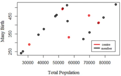
is the center of cluster 2 with 5 members, and so on, the center of cluster 5 is the 15-th record that has 2 members. The plot of two dimensions of dataset1 in radius r = 0.8 using two attributes X4 (Population number) and X5 (Many Births) are given in Figure 5 below.
Figure 5. Plot Cluster Center Versus Cluster Members of X4 to X5 on Dataset1
The Ctm of clustering results in the dataset2 (columns 3 and 4 of Table 5), the optimal cluster occurs at radius r = 0.45. Because on this radius, each cluster has at least 2 members and also has the smallest Ctm value is 0.33. The optimal center and cluster members of the dataset2 are presented in Table 7.
Table 7. The Optimal Cluster Center of Dataset2 and its Cluster Members
Cluster
Label Center
Cluster Members
X1 X2 X3 X4 X5
1 98.
88 91.37 53.15 7.07 90.47 8, 10, 18, 24 1, 3, 5, 7,
2 98.
66 96.
4 75.
05 9.89
97. 96
15, 30, 31, 32, 35, 36, 37
3 98.
58 94.
8 63.
57 8.04
94. 22
4, 6, 16, 17, 25, 34, 38
4 97.
91 80.44 42.35 6.79 83.1 9, 12, 13, 26
5 98.
26 88. 33
60.
88 6.24
84. 1
11, 14, 22, 23, 28, 33
6
97. 32
85. 34
42. 21 4.05
74.
4 27, 29
7
99. 57
98. 85
66. 91 7.46
87.
72 2, 19, 20, 21
[image:8.612.108.284.344.425.2]3725
Figure 6. Plot Cluster Center Versus Cluster Members of X2 to X5 on Dataset2
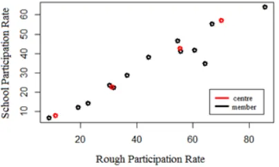
The Ctm of clustering results in dataset3 (columns 5 and 6 of Table 5), optimal clusters occur at radius r = 0.07. Because on this radius, each cluster has at least 2 members and also has the smallest Ctm value is 0.39. The optimal center and cluster members of dataset3 are presented in Table 8.
Table 8. The Optimal Cluster Center of Dataset3 and its Cluster Members
Cluster Label
Center Cluster
Members
X1 X2 X3
1 55.39 38.07 42.7 5,7,8,14,15,18,19 2 31.12 21.52 22.79 2,3,10,17 3 11.16 5.62 8.1 1,4,11,12 4 70.13 51.92 57.12 6,9,13,16
The plot of two-dimensional data with the center of the cluster at radius r = 0.07 for the variable used is X1 (Participation rate) and X3 (School Participation Rate) is presented in Figure 7 as follows:
Figure 7. Plot Cluster Center Versus Cluster Members of X1 to X3 on Dataset3
Based on the above description it has been shown that in the dataset1 having a large difference in covariance value or the variability between attributes is high obtained the radius parameters which yield optimal clustering is r=0.8. In the dataset2 with the difference of covariance matrix
between the variables that are not too large or variability between attributes of moderate values obtained radius parameters that yield optimal clustering of 0.45. In datasets3 which have almost homogeneous variance and covariance or variability between attributes are very small, the radius parameter that result in the optimal clustering are r= 0.07 which is almost close to zero.
Determination of the radius that produces optimal clustering cannot be done directly that must be done by trying some values. Based on the results obtained from this study to improve certainty in choosing the radius parameters in the Fsc method, it should be evaluated first against the covariance matrix between each attribute in the dataset. Information on the variability of the covariance matrix greatly affects the magnitude of the radius parameters. If a dataset has a very high variability then we should choose the size of the radius of a width that is between 0.7 to 0.9. This means that the more heterogeneous the objects to be clustered, the width of the radius is required as a filter for groups with a wide value. If the covariance matrix of a dataset has moderate variability, it is preferable to select the magnitude of the radius of about 0.5. Furthermore, on the other hand, if the covariance matrix of a dataset is relatively homogeneous, it is preferable that the radius parameter is selected small ie the magnitude of the radius parameter is closer to zero.
Unfortunately in determining the magnitude of variability that is categorized as large, moderate or small of a dataset is not an easy task and is subjective. In this study, we have provided 3 datasets that have the variability of large, moderate and small, but in its implementation in determining the variability of the dataset to be grouped requires an experience of its own. At least that information about the importance of calculating the covariance matrix value and making the boxplot diagram of the dataset are the steps that should be taken before applying Fsc has never been encountered in the existing literature included in [13-17]. However, the results obtained in this study are still limited to the dataset with the number of variables and records that are small.
5. CONCLUSION
Here are some conclusions from this study, 1. Variability of covariance matrix can be known
[image:9.612.92.294.493.614.2]3726 occurs between attributes in a dataset will be clearly described if boxplot diagram is drawn from each attribute.
2. The variability of the covariance matrix on a dataset greatly affects the magnitude of the radius parameter that results in the optimal cluster in the Fsc method.
3. In the dataset 1, the parameter of the radius of a large value (0.8), dataset2 are generated by the radius of medium value (0.45), whereas in dataset3 the parameter of small radius (0.07) is generated.
REFRENCES:
[1] Lisa L. Harlow, The Essence Of Multivariate Thinking : Basic Themes And Methods, Lawrence Erlbaum Associates, Inc., New Jersey, 2005.
[2] Alvin C. Rencher, Methods Of Multivariate Analysis, 2nd ed, John Wiley & Sons, Inc., Canada, 2002.
[3] F. Husson, Sebastian Le, J. Pages, Exploratory Multivariate Analysis by Example Using R. Taylor and Francis Group, CRC Press, New York, 2011.
[4] DS. Modha, and W. Scott Spangler, "Feature weighting in k-means clustering", Machine learning , 52.3, 2003, pp. 217-237.
[5] JZ. Huang, MK. Ng, H. Rong, and Z. Li, “ Automated variable weighting in k-means type clustering”, IEEE Transactions on Pattern Analysis and Machine Intelligence, 27(5), 2005, pp. 657-668.
[6] Mustakim, “Centroid K-Means Clustering Optimization Using Eigenvector Principal Component Analysis”, Journal of Theoretical & Applied Information Technology, 95.15,
2017, pp. 3534-3542.
[7] AK. Jumaa, AA. Aysar, RR. Aziz, AA. Shaltooki, R. Swathi, D. Sreenivas, and A. Ahmad, “Protect Sensitive Knowledge In Data Mining Clustering Algorithm”, Journal of Theoretical And Applied Information Technology, 95(15), 2017, pp. 3422-3431.
[8] B. Sugiantoro, and M H. Kiswanto, "Analysis OF Email Content With K-Means Clustering For Profiling On Postfix Server", Journal of Theoretical And Applied Information Technology , 95.17, 2017, pp. 4103-4113.
[9] H. Rabbouch, F. Saâdaoui, and R. Mraihi, "Unsupervised video summarization using cluster analysis for automatic vehicles counting and recognizing", Neurocomputing
,260, 2017, pp.157-173.
[10] SL. Chiu, “Fuzzy model identification based on cluster estimation”. Journal of Intelligent & fuzzy systems, 2(3), 1994, pp. 267-278.
[11] S. Tafazoli, L. Mathieu, and X. Sun, "Hysteresis modeling using fuzzy subtractive clustering", International journal of computational cognition, 4(3), 2006, pp.
15-27.
[12] A. Ghosh, NS. Mishra, and S. Ghosh, "Fuzzy clustering algorithms for unsupervised change detection in remote sensing images",
Information Sciences, 181.4, 2011, pp.
699-715.
[13] AY. Chamzini, M. Razani, SH.Yakhchali, EK. Zavadskas,Z. Turskis, “Developing a fuzzy model based on subtractive clustering for road header performance prediction”, Automation in Construction, 35, 2013, pp.111-120.
[14] SH. Rouhani, A. Sheikholeslami, H. Hosseini, H. Kazemi, “Application of fuzzy subtractive clustering for optimal transient performance of automatic generation control”, IETE Journal of Research, 59(6), 2013, pp. 753-760.
[15] T. Ariadji, AF. Mayusha, NN. Nissa, KA. Sidarto, E. Soewono, “Optimization of Direction and Length of Horizontal Wells in Oil Field-X Using Fuzzy Substractive Clustering and Fuzzy Logic Methods”,
Modern Applied Science, 8(6), 2014, pp.
326-336.
[16] KM. Bataineh, M. Naji, and M. Saqer, "A Comparison Study between Various Fuzzy Clustering Algorithms", Jordan Journal of Mechanical & Industrial Engineering, 5(4 ),
2011, pp. 335-343.
[17] LA. Lisangan, A. Musdholifah, and S. Hartati, “Two Level Clustering for Quality Improvement using Fuzzy Subtractive Clustering and Self-Organizing Map”,
Indonesian Journal of Electrical Engineering and Computer Science, 15(2), 2015, pp.
373-380.
[18] DP. Nalurita, Mapping of Health Facilities in Tulungagung Regency with Cluster Analysis using Average Linkage Method with Mahalanobis Distance and Euclidian, Thesis, Universitas Brawijaya, Malang, Indonesia, 2016, Unpublised.
3727 [20] Y. Yuliantini, Grouping Education
3728
[image:12.612.90.496.102.609.2]Appendix A.
Table 3. Clustering Results for the Various Radius Values on Dataset2
Radius=0.4 Radius=0.45 Radius=0.5 Radius=0.6 Radius =0.7 rec cl dg
[1,] 1 1.00 [2,] 6 0.45 [3,] 1 0.53 [4,] 3 1.00 [5,] 1 0.63 [6,] 3 0.59 [7,] 10 1.00 [8,] 10 0.34 [9,] 4 1.00 [10,] 1 0.56 [11,] 5 0.21 [12,] 4 0.24 [13,] 4 0.38 [14,] 10 0.32 [15,] 2 1.00 [16,] 3 0.34 [17,] 3 0.61 [18,] 1 0.32 [19,] 6 1.00 [20,] 6 0.26 [21,] 6 0.22 [22,] 5 0.47 [23,] 5 0.25 [24,] 1 0.63 [25,] 3 0.35 [26,] 4 0.06 [27,] 7 1.00 [28,] 5 1.00 [29,] 7 0.08 [30,] 2 0.44 [31,] 2 0.41 [32,] 8 1.00 [33,] 9 1.00 [34,] 3 0.28 [35,] 2 0.45 [36,] 2 0.57 [37,] 2 0.53 [38,] 3 0.47
rec cl dg [1,] 1 1.00 [2,] 7 0.54 [3,] 1 0.60 [4,] 3 1.00 [5,] 1 0.70 [6,] 3 0.66 [7,] 1 0.19 [8,] 1 0.26 [9,] 4 1.00 [10,] 1 0.63 [11,] 5 0.29 [12,] 4 0.32 [13,] 4 0.47 [14,] 5 0.03 [15,] 2 1.00 [16,] 3 0.43 [17,] 3 0.68 [18,] 1 0.40 [19,] 7 1.00 [20,] 7 0.34 [21,] 7 0.30 [22,] 5 0.55 [23,] 5 0.33 [24,] 1 0.69 [25,] 3 0.44 [26,] 4 0.10 [27,] 6 1.00 [28,] 5 1.00 [29,] 6 0.14 [30,] 2 0.52 [31,] 2 0.50 [32,] 2 1.00 [33,] 5 0.01 [34,] 3 0.37 [35,] 2 0.53 [36,] 2 0.64 [37,] 2 0.60 [38,] 3 0.55
rec cl dg [1,] 1 1.00 [2,] 3 0.29 [3,] 1 0.67 [4,] 3 1.00 [5,] 1 0.75 [6,] 3 0.71 [7,] 1 0.26 [8,] 1 0.34 [9,] 4 1.00 [10,] 1 0.69 [11,] 5 0.37 [12,] 4 0.40 [13,] 4 0.54 [14,] 5 0.06 [15,] 2 1.00 [16,] 3 0.50 [17,] 3 0.73 [18,] 1 0.48 [19,] 3 0.11 [20,] 3 0.19 [21,] 5 0.08 [22,] 5 0.62 [23,] 5 0.41 [24,] 1 0.74 [25,] 3 0.52 [26,] 4 0.16 [27,] 4 0.00 [28,] 5 1.00 [29,] 4 0.09 [30,] 2 0.59 [31,] 2 0.57 [32,] 2 0.00 [33,] 5 0.02 [34,] 3 0.44 [35,] 2 0.60 [36,] 2 0.69 [37,] 2 0.66 [38,] 3 0.62
Rec cl dg [1,] 1 1.00 [2,] 4 1.00 [3,] 1 0.75 [4,] 4 0.42 [5,] 1 0.82 [6,] 1 0.53 [7,] 1 0.39 [8,] 1 0.47 [9,] 3 0.65 [10,] 1 0.77 [11,] 3 0.25 [12,] 3 0.31 [13,] 3 1.00 [14,] 1 0.14 [15,] 2 1.00 [16,] 1 0.60 [17,] 4 0.45 [18,] 1 0.60 [19,] 4 0.70 [20,] 4 0.50 [21,] 4 0.66 [22,] 1 0.41 [23,] 1 0.45 [24,] 1 0.81 [25,] 2 0.56 [26,] 3 0.31 [27,] 3 0.04 [28,] 1 0.22 [29,] 3 0.21 [30,] 2 0.69 [31,] 2 0.67 [32,] 2 0.00 [33,] 1 0.05 [34,] 2 0.47 [35,] 2 0.70 [36,] 2 0.78 [37,] 2 0.75 [38,] 2 0.30