Runtime and Space Complexity Comparison of the
various Association Algorithms
K. Fathima Bibi,
Research Scholar, Reg. No.:Ph.D_CB_Dec2012_0441, Dept. of Comp. Sc., Bharathiyar University,Coimbatore, TN, India
M. Nazreen Banu,
Ph.D Research Advisor,Professor, Dept. of Comp. Sc. & Engg, MAM College of Engineering,
Tiruchirappalli, TN, India
ABSTRACT
Data mining has become an indispensable technology for businesses and researchers in many fields. Discovering frequent itemsets is a key problem in important data mining applications. Typical association algorithms for solving this problem operate in a bottom-up, top-down and breadth-first search direction. The computation starts from frequent 1-itemsets (the minimum length frequent itemsets) and continues until all maximal (length) frequent itemsets are found. Algorithms perform well when all maximal frequent itemsets are short. However, performance drastically decreases when some of the maximal frequent itemsets are relatively long. This paper focuses on finding Maximum Frequent Set with the implementation of the APRIORI and the Dynamic Itemset Counting Algorithm (DIC) and a comparative study with Pincer Search Algorithm to select the fast algorithm for discovering the Maximum Frequent Set.
General Terms
Knowledge Discovery, Data Warehousing, Data Mining, Algorithms, Patterns.
Keywords
Maximum Frequent Set, Association, Classification, Clustering, Sequential, Outlier, Evolution.
1. INTRODUCTION
Data Warehousing: The database in a data warehouse is not the same as the databases used for transaction processing. Data warehouse databases are designed to analyze terabytes of data and millions of records. They are organized to allow better analysis by using special techniques.
Data Mining:
hot buzzword for a class of techniques that find patterns in data [1]
A user-centric, interactive process which
leverages analysis technologies and computing power
A group of techniques that find relationships that have not previously been discovered
Knowledge Discovery in Database (KDD) defined as “the non-trivial process of identifying valid, novel, potentially useful, and ultimately understandable patterns in data”. A key component of many data mining problems is formulated as follows. Given a large database of sets of items, discover all frequent itemsets (sets of items), where
a frequent itemset is one that occurs in at least a user-defined percentage (minimum support) of the database. The problem was first formulated by Agrawal et al. [2, 3, 4, 5, 6, 7, 8, 9] and is often referred to as the ``market-basket'' problem. In this problem, a set of items and a large collection of transactions which are subsets (baskets) of these items are given. The task is to find relationship between the presences of various items within those baskets.
2. METHODOLOGIES
Different methods or techniques are proposed based on which the hidden patterns are discovered. They are Association Analysis, Classification, Prediction, Cluster Analysis, Sequential Pattern Analysis, Outlier Analysis and Evolution Analysis.
2.1 Association Analysis
As defined by Agrawal et al.,
LetI = {i1, i2, ……., in} be a set of n binary attributes
called items.
Let D = {t1, t2,……., tm} be a set of transactions called
the database.
Each transaction in D has a unique transaction ID and contains a subset of the items in I.
An Association rule is defined as an implication of the form X => Y where X, Y I and X ∩ Y =
ɸ
.
The sets of items (for short itemsets) X and Y is called antecedent (Left-Hand-Side or LHS) and consequent (Right-Hand-Side or RHS) of the rule.
{i1, i2} => {i3} means, if i1 and i2 are bought customers also buy i3.
The best-known constraints are minimum thresholds on support and confidence.
Support (Supp(X)) of an itemset X - the proportion of transactions in the data set which contain the itemset. Supp(X) = Number of transactions in which X occurred / Total number of transactions.
Confidence of a rule –
Conf(X => Y) = supp(X U Y) / supp(X).
7
2.2 Frequent Itemsets - Structural
Properties and Basic Discovery
Approaches
2.2.1 Maximum Frequent Set
Among all the frequent itemsets, some will be maximal frequent itemsets; they have no proper supersets that are themselves frequent. The maximum frequent set (or MFS) is the set of all the maximal frequent itemsets. The problem of discovering the frequent set can be reduced to the problem of discovering the MFS.
2.2.2 Closure Properties
The set of all itemsets is partitioned, perhaps implicitly, into three sets:
1. Frequent: This is the set of those itemsets that have been discovered so far as frequent. 2. Infrequent: This is the set of those itemsets that
have been discovered so far as infrequent. 3. Unclassified: This is the set of all the other
itemsets.
Initially, the frequent and the infrequent sets are empty. Throughout the execution, they grow at the expense of the unclassified set. The execution terminates when the unclassified set becomes empty, and then, of course all the maximal frequent itemsets are discovered.
Two closure properties can be used to immediately classify some of the unclassified itemsets
Property 1: If an itemset is infrequent, all it supersets must be infrequent, and they need not be examined further.
Property 2: If an itemset is frequent, all its subsets must be frequent, and they need not be examined further.
2.2.3 Discovering Frequent Itemsets
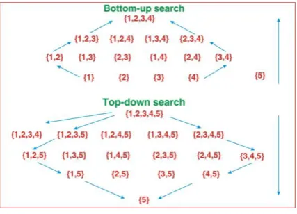
In general, it is possible to search for the maximal frequent itemsets either bottom-up or top-down. If all maximal frequent itemsets are expected to be short (close to 1 in size), it seems efficient to search for them bottom-up, uses only Property 1 to reduce the number of candidates. If all maximal frequent itemsets are expected to be long (close to n in size) it seems efficient to search for them top-down, uses only Property 2 to reduce the number of candidates as shown in Fig.1.
Bottom-up approach: It consists of repeatedly applying a pass, itself consisting of two steps. At the end of pass k all frequent itemsets of size k or less have been discovered. As the first step of pass k+1, itemsets of size k+1 each having two frequent k-subsets with the same first k-1 items are generated. Itemsets that are supersets of infrequent itemsets are pruned (and discarded), as of course they are infrequent (by Property 1). The remaining itemsets form the set of candidates for this pass. As the second step, the support of the candidates is computed (by reading the database), and they are classified as either frequent or infrequent.
Top-down approach: Starts with the single n-itemset and decreases the size of the candidates by one in every pass. When a k-itemset is determined to be infrequent, all of its (k-1)-subsets will be examined in the next pass. However,
[image:2.595.328.542.97.251.2]if a k-itemset is frequent, then all of its subsets must be frequent and need not be examined.
Fig. 1: Top-Down and Bottom-Up Searches
3. ASSOCIATION RULE MINING
ALGORITHMS
3.1 Apriori Algorithm
The Apriori algorithm is a typical bottom-up approach algorithm. The Apriori algorithm repeatedly uses Apriori-gen algorithm to Apriori-generate candidates and then count their supports by reading the entire database once. Apriori-gen relies on Property 1.
3.1.1 Join and Prune Procedures
The candidate generation algorithm consists of a join procedure and a prune procedure. The join procedure combines two frequent k-itemsets, which have the same (k-1) prefix, to generate a (k+1)-itemset as a new preliminary candidate. Following the join procedure, the prune procedure is used to remove from the preliminary candidate set all itemsets C such that some k-subset of C is not a frequent itemset.
The join procedure of the Apriori-gen algorithm
Input: Lk, the set containing frequent itemsets found in
pass k
Output: Preliminary candidate set Ck+1
The prune procedure of the Apriori-gen algorithm
Input:Preliminary candidate set Ck+1 generated from the
join procedure
Output: Final candidate set Ck+1, which does not contain
any infrequent subset
3.1.2 Reducing the Number of Candidates and
the Number of Passes
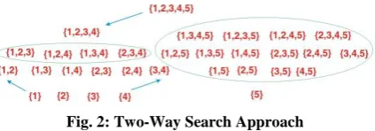
if an infrequent itemset is found in the bottom-up direction, then it can be used to eliminate some candidates in the top-down direction (Property 1). This “Two-Way Search Approach” shown in Fig.2 can fully make use of
Fig. 2: Two-Way Search Approach
both properties and thus speed up the search for the maximum frequent set. Reducing the number of candidates is of critical importance for the efficiency of the frequent set discovery process, since the cost of the entire process comes from reading the database (I/O time) to generate the supports of candidates ( CPU time) and the generation of new candidates (CPU time).
3.2 The Basic Pincer-Search Algorithm
The Pincer-Search Algorithm relies on the combined approach for determining the maximum frequent.
3.2.1 Pincer-Search Procedure
Input: A database and a user-defined minimum support Output: MFS, which contains all maximal frequent itemsets
The MFCS is initialized to contain one itemset, which consists of all the database items. The MFCS is updated whenever new infrequent itemsets are found. If an itemset in the MFCS is found to be frequent, then its subsets will not participate in the subsequent support counting and candidate set generation steps.
Pincer-Search reduces both the number of candidates and the number of passes.
3.2.1.1 Two-Way Search by Using the
MFCS
The two-way search algorithm for discovering the maximum frequent set relies on a new data structure during its execution, the maximum frequent candidate set (MFCS).
Consider some point during the execution of an algorithm for finding the MFS.
Let FREQUENT be the set of the itemsets known to be frequent.
Let INFREQUENT be the set of the itemsets known to be infrequent.
Then the maximum frequent candidate set (MFCS) is the minimum cardinality set of items satisfying the conditions.
FREQUENT U {2X / x MFCS}
INFREQUENT ∩ {2X / x MFCS} =
MFCS is a superset of the MFS. When the algorithm terminates, the MFCS and the MFS are equal. The computation of the algorithm follows the bottom-up breadth-first search approach.
In each pass, in addition to counting supports of the candidates in the bottom-up direction, the algorithm also counts supports of the itemsets in the MFCS; this set is adapted for the top-down search. This will help in pruning candidates, but will also require changes in candidate generation. The subsets of the MFCS must not contain this infrequent itemset.
By using the MFCS some maximal frequent itemsets may be discovered in early passes. This early discovery of the maximal frequent itemsets can reduce the number of candidates and the passes of reading the database, which in turn can reduce the CPU time and I/O time. This is especially significant when the maximal frequent itemsets discovered in the early passes are long.
3.2.1.2 Updating the MFCS
Replace every such itemset (say X) by Y itemsets, each obtained by removing from X a single item (element) of Y.
3.2.2 Procedure of MFCS-gen
Input: Old MFCS and the infrequent set Sk found in pass k
Output: New MFCS
3.2.3 Prune procedure
Input: Current MFCS and Ck+1 after join and recovery
procedures
Output: Final candidate set Ck+1
3.2.4 Candidate generation procedure
Input: Lk, current MFCS, and current MFS
Output: New candidate set Ck+1
3.3 The Dynamic Itemset Counting
Algorithm
1. Mark the empty itemset with a solid square. Mark all the 1-itemsets with dashed circles. Leave all other itemsets unmarked.
2. While any dashed itemsets remain:
Read M transactions (when the end of the transaction file is reached, continue from the beginning). For each transaction, increment the respective counters for the itemsets that appear in the transaction and are marked with dashes.
If a dashed circle's count exceeds minsupp, turn it into a dashed square. If any immediate superset of it has all of its subsets as solid or dashed squares, add a new counter for it and make it a dashed circle.
Once a dashed itemset has been counted through all the transactions, make it solid and stop counting it.
9 counting and exceeds the support
threshold minsupp.
Solid circle: confirmed infrequent itemset – that has finished counting and it is below minsupp.
Dashed square: suspected frequent itemset - an itemset which is still in counting that exceeds minsupp.
Dashed circle: suspected infrequent itemset - an itemset which is still in counting that is below minsupp.
Operations:
1. Add new itemsets
2. Maintain a counter for every itemset 3. Manage itemset states from dashed to solid
and from circle to square. When itemsets become large, determine which new itemsets should be added because they could potentially be large.
4. PERFORMANCE EVALUATION
Assume support to be equal to 20%. Since the number of transactions is 15, it means that an itemset is supported by at least three transactions is a frequent set. Generate candidate itemsets and frequent itemsets, when minimum support count is >2.
Table 1: Sample Database
Apriori Algorithm
In a 9 x 15, in pass -3 only one set is present. This is MFS. So the algorithm stops.
Pincer-Search Algorithm
Here also in pass -3 only one set is present which is MFS so the algorithm stops.
Dynamic Itemset Counting Algorithm
This algorithm requires only 2.75 database passes instead of 3 passes.
For the association mining algorithms to be effective, the top-down search needs to reach the maximal frequent itemsets faster than the bottom-up search.
5. TIME and SPACE COMPLEXITY
COMPARISON
Since transactions of itemsets are divided into groups by interval value, the work done by DIC algorithm [10] is increased. So complexity also increases. But the time taken to complete the algorithm is reduced.
In PINCER SEARCH algorithm, top-down and bottom-up approaches are applied on each step to find frequent itemset implicitly. So the amount of work done is increased in this case.
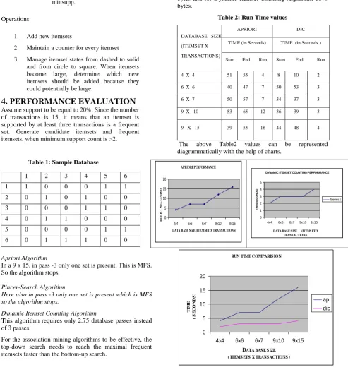
[image:4.595.130.294.71.242.2]If the amount of transactions and itemsets are increased, then considerably time taken to complete the process will be increased. The program size of Apriori algorithm is 923 bytes and for Dynamic Itemset Counting Algorithm 1879 bytes.
Table 2: Run Time values
DATABASE SIZE
(ITEMSET X
TRANSACTIONS)
APRIORI DIC
TIME (in Seconds) TIME (in Seconds )
Start End Run Start End Run
4 X 4 51 55 4 8 10 2
6 X 6 40 47 7 50 53 3
6 X 7 50 57 7 34 37 3
9 X 10 53 65 12 36 39 3
9 X 15 39 55 16 44 48 4
The above Table2 values can be represented diagrammatically with the help of charts.
RUN TIME COMPARIS ION
0 5 10 15 20
4x4 6x6 6x7 9x10 9x15
DATA BAS E S IZE
( ITEMS ETS X TRANS ACTIONS)
TI
M
E
( S
E
C
O
N
D
S
)
[image:4.595.76.570.233.760.2]ap dic
Fig. 3: Runtime and Space Complexity Comparison
APRIORI PERFORMANCE
0 5 10 15 20
4x4 6x6 6x7 9x10 9x15
DATA BASE SIZE (ITEMSET X TRANSACTIONS)
TI
M
E
(
S
EC
O
N
D
S
)
DYNAMIC ITEMSET COUNTING PERFORMANCE
0 1 2 3 4 5
4x4 6x6 6x7 9x10 9x15
DATA BAS E S IZE (ITEMS ET X TRANS ACTIONS )
T
IM
E
(S
E
C
O
N
D
S
)
Series1
6. CONCLUSION
The maximum frequent set provides a unique representation of all the frequent set, and once it is known, all the required frequent subsets can be easily generated. The Dynamic Itemset Counting algorithm could reduce both the number of times the database is read and the number of candidates.
Experiments show that the improvement of using this approach can be very significant, especially when some maximal frequent itemsets are long.
7. FUTURE ENHANCEMENTS
The performance of the Dynamic Itemset Counting algorithm in applications of discovering price changing patterns in stock market can be studied. It is worthwhile to study the performance of the Dynamic Itemset Counting Algorithm on problems having long maximal frequent itemsets. If the maximal frequent itemsets are distributed in a scattered manner, then the problem of discovering the MFS can be very hard. In this case, even Dynamic Itemset Counting Algorithm might not be able to solve it efficiently. Parallelizing the Dynamic Itemset Counting algorithm might be a possible way to solve this hard problem. The candidate set is divided in such a way that all the candidates that are subsets of an itemset in the MFCS are assigned to a same processor. Each processor can run totally independent. The issues to study would be the way to minimize the duplicate calculations and to maximize the use of available processors.
8. REFERENCES
[1] www.dama-ncr.org
[2] R. Agrawal, T. Imilienski, and A. Swami. Database Mining: A Performance Perspective. IEEE Transactions on Knowledge and Data Engineering, 5(6):914--925, December 1993.
[3] R. Agrawal, T. Imilienski, and A. Swami. Mining Association Rules between Sets of Items in Large Databases. Proc. of the ACM SIGMOD Int'l Conf. on Management of Data, pages 207--216, May 1993. [4] R. Agrawal and R. Srikant. Fast algorithms for
mining association rules. In Proceedings of the 20th VLDB Conference, Santiago, Chile, 1994.
[5] R. Agrawal and R. Srikant. Mining sequential patterns. In Proceedings of the 11th International Conference on Data Engineering, Taipei, Taiwan, 1995.
[6] R. Agrawal, K. Lin, S. Sawhney, and K. Shim. Fast similarity search in the presence of noise, scaling and translation in time-series databases. In Proc. of the Int'l Conf. on Very Large Data Bases (VLDB), 1995. [7] R. Srikant and R. Agrawal. Mining generalized
association rules. 1995.
[8] M. Mehta, R. Agrawal, and J. Rissanen. Sliq: A fast scalable classifier for data mining. March 1996. [9] H. Toivonen. Sampling large databases for
association rules. Proc. of the Int'l Conf. on Very Large Data Bases (VLDB), 1996.
[10] Sergey Brin, Rajeev Motwani y Jeffrey D. Ullman z, Dynamic Itemset Counting and Implication Rules for Market Basket Data, Department of Computer Science, Stanford University, Shalom Tsur, R&D Division, Hitachi America Ltd.