EKC: Static or Dynamic?

Munich Personal RePEc Archive

EKC: Static or Dynamic?

Dinda, Soumyananda

S. R. Fatepuria College, Beldanga, Murshidabad, West B, India,

Economic Research Unit, Indian Statistical Institute, 203, B. T.

Road, Kolkata-108, India.

2006

Online at

https://mpra.ub.uni-muenchen.de/65159/

EKC: Static or Dynamic?

Soumyananda Dinda*

Economic Research Unit, Indian Statistical Institute, 203, B. T. Road, Kolkata-108, India. S. R. Fatepuria College, Beldanga, Murshidabad, West B, India.

Abstract

This paper tests the robustness of the Environmental Kuznets Curve (EKC) hypothesis, using dynamic model specification for the long panel data set rather than static model. The monotonic income - CO2

emission relationship exists in most of the under developed or developing economies but EKC exists mostly in developed economies.

JEL

Classification Number

: C33, Q25.

Kay words

: EKC, Dynamic model, CO

2

Emission.

---*Corresponding Author: C/o, Dipankor Coondoo, Economic Research Unit, Indian Statistical Institute, 203, B. T. Road, Kolkata-35. E-mail: [email protected] or [email protected].

1.

Introduction

This paper investigates the robustness of the Environmental Kuznets Curve (EKC), an inverted-U shaped relationship between environmental quality indicators1 and the level of economic activity or income. Several earlier studies (See, Grossman and Krueger 1995, Selden and Song 1994, de Bruyn et al. 1998, Holtz-Eakin and Selden 1995, Cole et al. 1997, Dinda et al. 2000, Shafik 1994, etc.) have attempted to test the EKC hypothesis empirically with the help of panel data. Most of these studies have used static model for estimation purpose. Little attention has been given in the model specification, especially dynamic model specification in the EKC literature.

In re-examining the EKC relationship, this study improves over the previous literature in two aspects. Firstly, proper selection of a model and appropriate method of estimation are important for panel data. A dynamic model helps to draw a valid inference about the parameters of the EKC relationship. Finally, we re-examine the validity of EKC relationship between CO2 emission and

income using a cross-country panel data covering 88 countries, which are taken from all the continents of the world over the period 1960 - 1990.

In the next section, we select an appropriate model, the empirical results are analyzed in section 3, and a summary of the findings is given in the final section.

2. Methodology and Model selection

The basic simple EKC model, is used by most of the earlier studies, is given as:

it it it

i

it

T

x

x

y

=

α

+

φ

+

β

₁

+

β

₂ 2

+

ε

(1)

Where

y

_it denotes the environmental quality indicator of ith individual at time t; x is income per capita (PPP at a constant price, 1985),

α

_iis the country specific effect, T is the time trend and

ε

_it is

1

disturbance term. Note that this model has an individual effect (

α

_i) that allows for the intercept of the

Kuznets curve to vary in every country. Despite the inclusion of fixed country effects, the

β

s, which measures the effect of the explanatory variables, is the same for each country for each time period. The parameter

β

s can be thought of as the average income - emission relation, but individual country may differ from this average. Actually, equation (1) is a static model. It means that due to any shock, all adjustment takes place within the time period in which it occurs. Here adjustment process is actually instantaneous. On the contrary, a slow adjustment process exists in reality and a statistical sound approach is required to estimate a dynamic model (see Greene 1998) in panel data set up. The earlier EKC models are mis-specified because the dynamic nature of the model has not been taken into consideration for the estimation purpose in case of long time series data in panel set up. Now, we consider the following dynamic model:

it it it

it i

it

T

y

x

x

y

=

α

+

φ

+

η

₋₁

+

β

₁

+

β

₂ 2

+

ε

′

(2)

This dynamic relationship is characterized by the presence of a lagged dependent variable among the regressors. Thus, autocorrelation effect can be removed from error terms.

3. Data and discussion of results

For the present study, we have used cross-country panel data on per capita GDP (PCGDP, measured at 1985 US dollar) compiled by Summers and Heston (Mark 5.6) and corresponding per capita CO2

emission (PCCO2, measured in metric tons) are taken from Carbon Dioxide Analysis Information Center (CDAIC) of Oak Ridge National Laboratory (ORNL), USA. Given these basic data, we have compiled a cross-country bi-variate panel data set of yearly observations covering 88 countries spread over the globe for the time period 1960 - 1990.

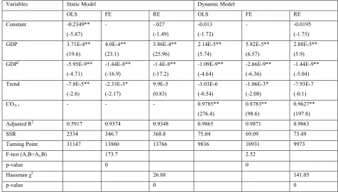
Now, we see the results of static model (1). The estimated turning point for the global EKC is $31147 (at US 1985 Prices) per capita income which is the out of sample range, that imply a monotonic income-emissions relation. This estimated turning point is nearly same as that of Holtz-Eakin and Selden (1995) (i.e., $35428 per capita). The estimates are consistent with an inverted-U shape for the CO2 emission-income relation (i.e.,

β

₁>0 and

β

₂<0). In most of the developed

countries, CO2 emission starts to decline after oil shock (see, Moomaw and Unruh (1997)).

Incorporating dummy (d=1 for post oil shock period, i.e., 1975 1990, and zero otherwise, i.e., 1960 -1974) in model 1 and 2, we also try to examine the oil shock effect which is the major cause of reducing CO2 emission in post oil shock period. We also examine the EKC relationship between

income and emission for individual countries. Table 1 presents the results of individual EKC regressions. In case of with and without trend, the statistically significant EKCs exist in 34 and 36 countries out of 88, respectively. The relationship of CO2 emission with per capita income has been

found to be monotonic in most of the under developed and developing economies but EKC exists mostly in developed economies (see table 1).

general for the world, these results reject the monotonic relationship of carbon dioxide emission with per capita income. The estimated Turning Point of global EKC model differs from OLS to FE or RE model estimations (See Table 2).

In general, the valid inference can be drawn about the parameters of the EKC relationship between PCGDP and PCCO2 when a more completely specified dynamic model (i.e., equation (2)) is chosen. Now, for the model (2), we obtain the turning point at $10931 per capita in FE model estimation and in OLS at $ 9836 per capita, which is far below that of model (1). The model (1) is mis-specified because the dynamic effect has not been considered in long panel data. The dynamic effects have been incorporated in the model (2). The results are drastically changed if the model is properly selected or specified. See the table 2, how the estimated results differ due to mis-specification of models. The result of dynamic model is consistent and efficient for EKC relationship.

4. Conclusion

Our findings are briefly: It makes an important difference for estimation and inference techniques in case of dynamic model rather than static model in case of panel data. The EKC relations exist for the world as a whole, and Carbon dioxide emission is no longer monotonic with per capita income. The FE estimation of dynamic model is consistent and efficient for global EKC relation. The individual EKC relation exists mostly for developed economies.

5. References

• Agras, J. and Chapman, D., 1999, A Dynamic Approach to the Environmental Kuznets Curve hypothesis, Ecological Economics, vol.-28, 267 - 277.

• Cole, M. A., A. J. Rayner and J. M. Bates, 1997, The Environmental Kuznets Curve: an empirical analysis, Environment and Development Economics, vol.-2, 401 - 416.

• de Bruyn, S. M., J. C. J. M. van den Bergh, and J. B. Opschoor, 1998, Economic growth and emissions: reconsidering the empirical basis of Environmental Kuznets Curve, Ecological Economics, vol.-25, 161 - 175.

• Dinda, S., D. Coondoo, and M. Pal, 2000, Air quality and economic growth: an empirical study,

Ecological Economics, vol.-34, 409 - 423.

• Grossman, G. M. and A. B. Krueger, 1995, economic growth and the environment, Quarterly journal of Economics, vol.-110, 353 - 377.

• Greene, W., 1998, Econometric Analysis, Prentice-Hall International, Inc.

• Holtz-Eakin, D. and T. M. Selden, 1995, Stoking the fires? CO2 emissions and economic growth,

Journal of Public Economics, vol.-57, 85 - 101.

• Hsiao, C., 1986, Analysis of panel data, Cambridge University Press, New York, (reprint 1989).

• Moomaw, W. R. and G. C. Unruh, 1997, are environmental kuznets curves misleading us? The case of CO2 emissions, Environment and Development Economics, vol.-2, 451 - 463.

• Selden, T. M. and D. Song, 1994, Environmental quality and development: Is there a kuznets curve for air pollution emissions?, Journal of Environmental economics and Management, vol.-27, 147 - 162.

• Shafik, N., 1994, Economic development and environmental quality: An econometric analysis,

[image:5.612.92.510.195.274.2]

Table 1: Results of individual EKC regression: with and without trends.

OECD Non-OECD

With trend Without trend With trend Without trend

1

β

>0 and

β

₂<0 (EKC) 20/27 18/27 14/61 18/61

1

β

<0 and

β

₂>0 (U-shaped) 2/27 1/27 5/61 4/61

Table 2: Estimated EKC results for Static and Dynamic models.

Variables Static Model Dynamic Model

OLS FE RE OLS FE RE

Constant -0.2349** (-5.87) - -.027 (-1.49) -0.013 (-1.72) - -0.0195 (-1.75) GDP 3.71E-4** (19.6) 4.0E-4** (23.1) 3.86E-4** (25.96) 2.14E-5** (5.74) 5.82E-5** (6.57) 2.88E-5** (5.9)

GDP2 _-5.95E-9**

(-4.71) -1.44E-8** (-16.9) -1.4E-8** (-17.2) -1.09E-9** (-4.64) -2.66E-9** (-6.36) -1.44E-9** (-5.04) Trend -7.8E-5** (-2.6) -2.33E-3* (-2.17) 9.9E-5 (0.83) -3.03E-6 (-0.54) -1.06E-3* (-2.08) -7.93E-7 (-0.1)

CO2t-1 - - - 0.9785**

(276.4)

0.8783**

(98.6)

0.9627**

(197.8)

Adjusted R2 _{0.5917 0.9374 0.9348 0.9865 0.9871 0.9863}

SSR 2334 346.7 360.8 75.04 69.09 73.49

Turning Point 31147 13860 13766 9836 10931 9973

F-test (A,B=Ai,B) 173.7 2.52

p-value 0 0

Hausman χ2 _{26.88 141.05}

p-value 0 0

Note: Figures in parentheses are t-ratios. SSR= Sum of Squared Residuals. * and ** denote the significance level at 5% and 1%,

[image:5.612.69.545.396.667.2]