Mixed Transforms Generated by Tensor Product and
Applied in Data Processing
Saifuldeen A. Mohammed
M.Sc LecturerElectrical Department College of Engineering Baghdad University
Zainab Ibraheem
M.Sc Assistant LecturerElectrical Department College of Engineering, Baghdad University
Abdullah Abdali Jassim
B.Sc in Computer EngineeringHead of IT Academies, Computer Center, Baghdad University
ABSTRACT
Finding orthogonal matrices in different sizes is very complex and important because it can be used in different applications like image processing and communications (e.g. CDMA and OFDM). In this paper we introduce a new method to find orthogonal matrices by using tensor products between two or more orthogonal matrices of real and imaginary numbers with applying it in images and communication signals processing. The output matrices will be orthogonal matrices too and the processing by our new method is very easy compared to other classical methods those use basic proofs .The results are normal and acceptable in communication signals and images but it needs more research works.
General Terms
Mixed Transforms, Tensor Operation, Orthogonal Matrices, Images Compression, Communication system.
Keywords
Orthogonally, OFDM, CDMA, JCDMA, Wavelet, Safe Transform, Compression, Kronecker product.
1.
INTRODUCTION
The definition of the matrix that it is orthogonal can be summary by the equations below [1]:
Anxn∗ A∗Tnxn= Inxn Or Anxn∗ A∗Tnxn= kInxn then: Anxn−1 =
A∗Tnxn or Anxn−1 = A∗Tnxn⁄ k .
Where k is a constant, A is square matrix and I identical squa-re matrix (the main diagonal is one) example:
FFT4×4∗ FFTm4×4∗T =(
1 1 1 1 1 −j −1 j 1 −1 1 −1 1 j −1 −j
)∗(
1 1 1 1 1 −j −1 j 1 −1 1 −1 1 j −1 −j
)
=(
4 0 0 4
0 0 0 0 0 0 0 0
4 0 0 4
)= 4 ∗(
1 0 0 1
0 0 0 0 0 0 0 0
1 0 0 1
)
= 4 ∗ I4×4
Where k is any constant number (may be real or imaginary), the conjugate transport for the matrix for both real and imaginary matrices like FFTn×n matrix, let us take Fast Fourier Transform matrix 4×4 size , Walsh Hadamared and Safe 4×4 transforms as in the following example[1],
The first FFTn×n :
FFTm4×4= (
1 1 1 1 1 −j −1 j 1 −1 1 −1 1 j −1 −j )
The second Walsh Hadamared: If Walsh Hadamared 2x2 is equal:
WH2×2= (1 11 −1)
Then the 4x4 tensor product will be:
WH4×4= WH2×2WH2×2= (1 11 −1)(1 11 −1)
= (WH2×2 WH2×2
WH2×2 −WH2×2)
= (
1 1 1 1 1 −1 1 −1 1 1 −1 −1 1 −1 −1 1 )
And the third, Safe Transform 𝕊nxnθ where n is the dimension
and θ is the phase shift, let n=2 and θ=0o then:
𝕊2x2= (−1 −j ) j 1 , And 𝕊2nx2nθ = WH2×2 𝕊nxnθ or
𝕊4𝑥4= WH2×2𝕊2x2= (𝕊2x2 𝕊2x2
𝕊2x2 −𝕊2x2
) =
𝕊4𝑥4= (1 11 −1)(−1 −j) = ( j 1
j 1
−1 −j −1 −j j 1 j 1
−1 −j 1−j −1 j )
2.
BASIC MATHEMATICS
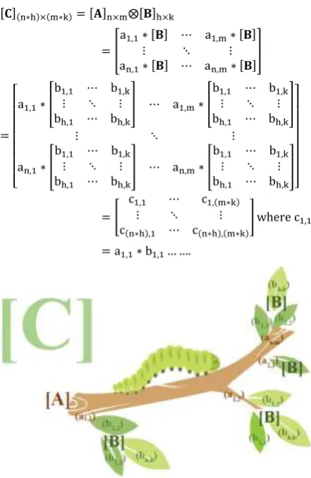
We find that for Walsh Hadamard and Safe Transform can be created by tensor product, the question is what is the tensor product? It is like a tree has branches and the branches have leaves (see Figure 1) or a basic victor in its end has many a new vectors where:
[𝐀]n×m= [
a1,1 ⋯ a1,m
⋮ ⋱ ⋮
an,1 ⋯ an,m
]
[𝐁]h×k= [
b1,1 ⋯ b1,k
⋮ ⋱ ⋮
bh,1 ⋯ bh,k
Volume 81– No.19, November 2013 [𝐂](n∗h)×(m∗k)= [𝐀]n×m⨂[𝐁]h×k
= [
a1,1∗ [𝐁] ⋯ a1,m∗ [𝐁]
⋮ ⋱ ⋮
an,1∗ [𝐁] ⋯ an,m∗ [𝐁]
]
=
[ a1,1∗ [
b1,1 ⋯ b1,k
⋮ ⋱ ⋮
bh,1 ⋯ bh,k
] ⋯ a1,m∗ [
b1,1 ⋯ b1,k
⋮ ⋱ ⋮
bh,1 ⋯ bh,k
]
⋮ ⋱ ⋮
an,1∗ [
b1,1 ⋯ b1,k
⋮ ⋱ ⋮
bh,1 ⋯ bh,k
] ⋯ an,m∗ [
b1,1 ⋯ b1,k
⋮ ⋱ ⋮
bh,1 ⋯ bh,k
] ]
= [
c1,1 ⋯ c1,(m∗k)
⋮ ⋱ ⋮
c(n∗h),1 ⋯ c(n∗h),(m∗k)
] where c1,1
[image:2.595.54.275.68.407.2]= a1,1∗ b1,1… ….
Fig 1: Kronecker tensor product
The tensor product, may be applied in different ways in vectors, matrices, spaces, algebras, topological vector and modules, among many other structures or objects. The most general bilinear operation, in some contexts, this product is also referred to as outer product. The linear maps A and B can be represented by matrices. Then, the description of matrix tensor product is the Kronecker product of the two or more matrices. There are many properties for tensor product but in this paper we will proof a new property that can be applied for our research, the property is:
Theorem 1 If A: → and B: → are square matrices, and both A and B are orthogonal matrices then action of their tensor product on a matrix is given by (A⊗B=C: →) the matrix C will be square orthogonal too, which is the set for complex numbers including the vectors numbers.
Proof: We have that [𝐀]n×n= [
a1,1 ⋯ a1,n
⋮ ⋱ ⋮
an,1 ⋯ an,n
]
[𝐁]m×m= [
b1,1 ⋯ b1,m
⋮ ⋱ ⋮
bm,1 ⋯ bm,m
]
And both orthogonal or
𝐀nxn∗ 𝐀∗Tnxn= 𝐈nxn Or 𝐀nxn∗ 𝐀∗Tnxn= k1𝐈nxn then: 𝐀−1nxn=
𝐀∗Tnxn or 𝐀−1nxn= 𝐀∗Tnxn⁄ k1
And
𝐁mxm∗ 𝐁mxm∗T = 𝐈mxm Or 𝐁mxm∗ 𝐁mxm∗T = k2𝐈mxm then
: 𝐁mxm−1 = 𝐁mxm∗T or 𝐁mxm−1 = 𝐁mxm∗T ⁄ k1
Where both k1, k2 and
[𝐂](n∗m)×(n∗m)= [𝐀]n×n⨂[𝐁]m×m
= [
a1,1∗ [𝐁] ⋯ a1,n∗ [𝐁]
⋮ ⋱ ⋮
an,1∗ [𝐁] ⋯ an,n∗ [𝐁]
]
=
[ a1,1∗ [
b1,1 ⋯ b1,m
⋮ ⋱ ⋮
bm,1 ⋯ bm,m
] ⋯ a1,n∗ [
b1,1 ⋯ b1,m
⋮ ⋱ ⋮
bm,1 ⋯ bm,m
]
⋮ ⋱ ⋮
an,1∗ [
b1,1 ⋯ b1,m
⋮ ⋱ ⋮
bm,1 ⋯ bm,m
] ⋯ an,n∗ [
b1,1 ⋯ b1,m
⋮ ⋱ ⋮
bm,1 ⋯ bm,m
] ]
= [
c1,1 ⋯ c1,(n∗m)
⋮ ⋱ ⋮
c(n∗m),1 ⋯ c(n∗m),(n∗m)
] where c1,1= a1,1∗ b1,1… ….
As we now A*T⊗B*T = (A⊗B)*T = C*T then we must proof th
at C* C*T=kI
𝑘[𝐈](n∗m)×(n∗m)= [𝐂](n∗m)×(n∗m)∗ [𝐂](n∗m)×(n∗m)∗T
= ([𝐀]n×n⨂[𝐁]m×m) ∗ ([𝐀]n×n∗T⨂[𝐁]m×m∗T)
= [
a1,1∗ [𝐁] ⋯ a1,n∗ [𝐁]
⋮ ⋱ ⋮
an,1∗ [𝐁] ⋯ an,n∗ [𝐁]
] ∗ [
a1,1∗∗ [𝐁]∗T ⋯ an,1∗∗ [𝐁]∗T
⋮ ⋱ ⋮
a1,n∗∗ [𝐁]∗T ⋯ an,n∗∗ [𝐁]∗T
]
=
[ a1,1∗ [
b1,1 ⋯ b1,m
⋮ ⋱ ⋮
bm,1 ⋯ bm,m
] ⋯ a1,n∗ [
b1,1 ⋯ b1,m
⋮ ⋱ ⋮
bm,1 ⋯ bm,m
]
⋮ ⋱ ⋮
an,1∗ [
b1,1 ⋯ b1,m
⋮ ⋱ ⋮
bm,1 ⋯ bm,m
] ⋯ an,n∗ [
b1,1 ⋯ b1,m
⋮ ⋱ ⋮
bm,1 ⋯ bm,m
] ]
∗
[ a1,1∗∗ [
b1,1∗ ⋯ bm,1∗
⋮ ⋱ ⋮
b1,m∗ ⋯ bm,m∗
] ⋯ an,1∗∗ [
b1,1∗ ⋯ bm,1∗
⋮ ⋱ ⋮
b1,m∗ ⋯ bm,m∗
]
⋮ ⋱ ⋮
a1,n∗∗ [
b1,1∗ ⋯ bm,1∗
⋮ ⋱ ⋮
b1,m∗ ⋯ bm,m∗
] ⋯ an,1∗∗ [
b1,1∗ ⋯ bm,1∗
⋮ ⋱ ⋮
b1,m∗ ⋯ bm,m∗
] ]
If we take the first row to the [C] then we gate:
k ∗ 1 = a1,1a1,1∗ (b1,1b1,1∗ + b1,2b1,2∗ … … … b1,mb1,m∗ )
+a1,2a1,2∗ (b1,1b1,1∗ + b1,2b1,2∗ … … … b1,mb1,m∗ ) + … ..
… + a1,na1,n∗ (b1,1b1,1∗ + b1,2b1,2∗ … … … b1,mb1,m∗ )
k ∗ 1 = ∑ ((a1,i∗ a1,i∗ ) ∗ ∑(b1,j∗ b1,j∗ ) 𝑚
𝑗=1
)
𝑛
𝑖=1
Because [B] is orthogonal then:
(b1,1b1,1∗ + b1,2b1,2∗ … … … b1,mb1,m∗ ) = ∑𝑚𝑗=1(b1,j∗ b1,j∗ )= 1
𝑜𝑟 𝑘2 (Otherwise = 0) then the equations will be:
∑ ((a1,i∗ a1,i∗ ) ∗ ∑(b1,j∗ b1,j∗ ) 𝑚
𝑗=1
)
𝑛
𝑖=1
= (1 𝑜𝑟 𝑘2) ∑(a1,i∗ a1,i∗ ) 𝑛
𝑖=1
And because [A] is orthogonal too then the equation will be:
∑ ((a1,i∗ a1,i∗ ) ∗ ∑(b1,j∗ b1,j∗ ) 𝑚
𝑗=1
)
𝑛
𝑖=1
= (1 𝑜𝑟 𝑘2) ∗ (1 𝑜𝑟 𝑘1) = 𝑘
For the second row for [C] will be as:
0 = a2,1a1,1∗ (b1,1b1,1∗ + b1,2b1,2∗ … … … b1,mb1,m∗ )
+a2,2a1,2∗ (b1,1b1,1∗ + b1,2b1,2∗ … … … b1,mb1,m∗ ) + … …
… + a2,na1,n∗ (b1,1b1,1∗ + b1,2b1,2∗ … … … b1,mb1,m∗ )
0 = ∑ ((a2,i∗ a1,i∗ ) ∗ ∑(b1,j∗ b1,j∗ ) 𝑚
𝑗=1
)
𝑛
𝑖=1
Because ∑𝑚𝑗=1(b1,j∗ b1,j∗ )= (1 𝑜𝑟 𝑘2) but:
∑𝑛𝑖=1(at,i∗ al,i∗)= {0 if t ≠ l1 if t = l
This is the most desired property in the orthogonally applied
to the matrices; therefore [C] is orthogonal and square and:
𝑘[𝐈](n∗m)×(n∗m)= [
c1,1 ⋯ c1,(n∗m)
⋮ ⋱ ⋮
c(n∗m),1 ⋯ c(n∗m),(n∗m)
]
∗ [
c1,1∗ ⋯ c1,(n∗m)∗
⋮ ⋱ ⋮
c(n∗m),1∗ ⋯ c(n∗m),(n∗m)∗
]
where c1,1= a1,1∗ b1,1…
And this is the proof
As we shown it can create an orthogonal matrix from two or more orthogonal matrices as shown in the example below:
Example 1: Let [𝐀] = [1 1
1 −1] and Wavelet Db2 [𝐁] =
[ 1 1
0 0 01 1 0 1 −1
0 0 0 01 −1 ] then
[𝐀]2x2⨂[𝐁]4x4=
[
1 1 0 0 1 1 0 0
0 0 1 1 0 0 1 1
1 −1 0 0 1 −1 0 0
0 0 1 −1 0 0 1 −1
1 1 0 0 −1 −1 0 0
0 0 1 1 0 0 −1 −1
1 −1 0 0 1 −1 0 0
0 0 1 −1 0 0 1 −1]
Then to proof the orthogonally:
[
1 1 0 0 1 1 0 0
0 0 1 1 0 0 1 1
1 −1 0 0 1 −1 0 0
0 0 1 −1 0 0 1 −1
1 1 0 0 −1 −1 0 0
0 0 1 1 0 0 −1 −1
1 −1 0 0 1 −1 0 0
0 0 1 −1 0 0 1 −1]
∗
[
1 0 1 0 1 0 1 0
1 0 −1 0 1 0 −1 0
0 1 0 1 0 1 0 1
0 1 0 −1 0 1 0 −1
1 0 1 0 −1 0 1 0
1 0 −1 0 −1 0 −1 0
0 1 0 1 0 −1 0 1
0 1 0 −1 0 −1 0 −1]
=
[ 4 0 0 4 0 00 0 0 0 0 0 4 00 4
0 0 0 0 0 00 0 0 0 0 0 0 00 0 0 0
0 0 0 00 0 0 0 0 0 0 00 0
4 0 0 4 0 00 0 0 0 0 0 4 00 4]
= 4[𝐈]8𝑥8
Example 2: Safe transform if we take 𝕊245o= [1 −jj −1] and
wavelet Db2[𝐁] = [
1 1
0 0 01 1 0 1 −1
0 0 0 01 −1 ] then:
𝕊245
o
⨂[𝐁] = [ 1 1
0 0 01 1 0 1 −1
0 0 0 01 −1
] ⨂ [1 −jj −1]
=
[
1 −j 1 −j 0 0 0 0
j −1 j −1 0 0 0 0
0 0 0 0 1 −j 1 −j
0 0 0 0 j −1 j −1
1 −j −1 j 0 0 0 0
j −1 −j 1 0 0 0 0
0 0 0 0 1 −j −1 j
0 0 0 0 j −1 −j 1]
= [𝐗]
Then [X]* [X]*T=4[I]
8x8(Where X from Mixed)
Example 3: [𝐁]⨂ 𝕊245
o
⨂𝐖𝐇𝟐= [𝐗]
=
[
1 −j 1 −j 0 0 0 0
j −1 j −1 0 0 0 0
0 0 0 0 1 −j 1 −j
0 0 0 0 j −1 j −1
1 −j −1 j 0 0 0 0
j −1 −j 1 0 0 0 0
0 0 0 0 1 −j −1 j
0 0 0 0 j −1 −j 1]
⨂ [−j −j−j j]
Then [X]* [X]*T=4[I]
16x16(Where X from Mixed).
3.
MIXED TRANSFORMS
In this section we will take several cases to find Mixed Transforms from two or more famous transforms like Wavelets Groups, Slantlet, Fourier Transform and other Transform (we will take the special case just in this paper). It can be create a Mixed Transforms from the following:
1- Wavelet with Wavelet its self ,
2- Wavelet with other family Wavelet ,
3- Slantlet With Wavelet family,
4- Fourier with Wavelet and Slantlet , .
.
At the end there are many of mixed two transforms or more the cause for this way to achieve the advantage for this transforms in one matrix or different sizes of filters to different sizes of objects and study the performances,
Volume 81– No.19, November 2013
Fig 2: 𝕊𝟐𝟒𝟓
𝐨
⨂[𝐁]⨂𝐖𝐇𝟐= [𝐗]
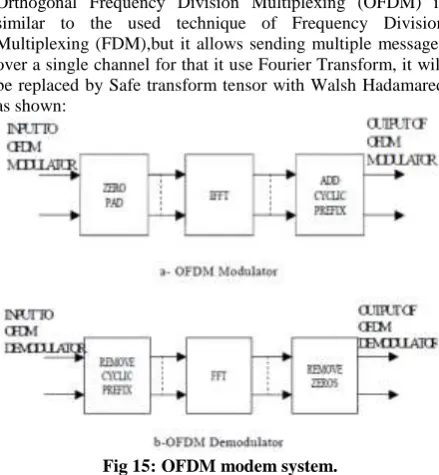
Fig 3: Old way Mix Algorithm for Images
Fig 4: New way Mix Algorithm for Images
4.
IMAGES APPLICATION
In this section, the images compression as most application in DSP today, in image processing there are 256 intensity levels (scales) of grey. 0 is black and 255 are white. Each level is represented by an 8-bit binary number so black is 00000000 and white is 11111111. An image can therefore be thought of as grid of pixels, where each pixel can be represented by the 8-bit binary value for grey-scale. Images require much storage space, large transmission bandwidth and long transmission time (and in the early year the storage devices were very expansive). The only way currently to improve these resource requirements is to compress images, such that they can be transmitted quicker and then decompressed by the receiver [4]. The compression is a process of representing information in a compact form with less bit rate for transmission or less storage while maintaining acceptable fidelity or data quality [10]. Image compression is a reduction method of the number of pixels needed to store a digital image [6]. The aim of image compression algorithms is to remove the redundancy in data in a way which makes image reconstruction possible." This basically means that image compression algorithms try to exploit redundancies in the data; they calculate which data
needs to be kept in order to reconstruct the original image and therefore which data can be ’thrown away’. By removing the redundant data, the image can be represented in a smaller number of bits, and hence can be compressed [4].
5.
COMPRESSION USING WAVELET
TRANSFORM
Wavelets are functions which allow data analysis of signals or images, according to scales or resolutions and it provide a powerful and remarkably flexible set of tools for handling fundamental problems in science and engineering, such as signal (image) compression, image de-noising, image enhancement, image recognition [9]. The wavelet transform is a type of signal transform that is commonly used in image compression [10], so, by using a wavelet image compression, the compressed image size is reduced but the quality of the image is quite similar to original image [9]. Wavelet analysis can be used to divide the information of an image into approximation and detail sub signals. The approximation sub signal shows the general trend of pixel values, and three detail sub signals show the vertical, horizontal and diagonal details or fast changes in the image [5]. In the decomposition level
=
[
1 1
1 −1
−j −j
−j j 11 −11
−j −j
−j j 00 00
0 0
0 0
0 0
0 0
0 0
0 0
j j
j −j −1−1 −11
j j
j −j −1−1 −11 00 00 00 00 00 00 00 00
0 0
0 0
0 0
0 0
0 0
0 0
0 0
0 0
1 1
1 −1
−j −j
−j j 11 −11
−j −j
−j j
0 0
0 0 00 00 00 00 00 00
j j
j −j −1−1 −11
j j
j −j −1−1 −11
1 1
1 −1
−j −j
−j j −1−1 −11
j j
j −j 00 00 00 00 00 00 00 00
j j
j −j −1−1 −11
−j −j
−j j 11 −11
0 0
0 0
0 0
0 0
0 0
0 0
0 0
0 0
0 0
0 0 00 00 00 00 00 00 11 −11
−j −j
−j j −1−1 −11
j j
j −j
0 0
0 0
0 0
0 0
0 0
0 0
0 0
0 0
j j
j −j −1−1 −11
−j −j
−j j 11 −1]1
First Transform Second
Transform Second
Transform First Transform
*T *T
2ed T 2ed T 2ed T 2ed T
2ed T 2ed T 2ed T 2ed T
2ed T 2ed T 2ed T 2ed T
2ed T 2ed T 2ed T 2ed T
2ed T *T
2ed T *T
2ed T *T
2ed T *T
2ed T *T
2ed T *T
2ed T *T
2ed T *T 2ed T
*T
2ed T *T
2ed T *T
2ed T *T
2ed T *T
2ed T *T
2ed T *T
one, the image will be divided into 4 sub-bands, called LL, LH, HL, and HH. The LL sub-band is a low-resolution residue that has low frequency components, which are often referred to as the average image, LH provides vertical detailed images, HL provides detailed images in the horizontal direction, finally, the HH sub-band image gives details on the diagonal, In the discrete wavelet transform (DWT), there are properties for precise reconstruction. This nature gives a sense that in fact no information is lost after the transformed image is set to its original form. But there are missing information on image data compression with wavelet transform that occurs during quantization. Information loss due to compression should be minimized to keep the quality of the compression. A good quality compression is generally achieved in the process of memory consolidation, which generates a small reduction, and vice versa. The quality of an image is subjective and relative, depending on the observation of the user [5]. Compression ratio is the ratio of number of bits required to represent the data before compression to the number of bits required to represent data after compression. Increase of compression ratio causes more effective compression technique employed and vice versa [7].
The energy measures pixel pair’s repetitions. For each sub-band, it is computed by using the equation below:
Energy=∑ ∑ P2(i, j)
Where P(i, j) is probability density and i and j are the gray levels [8].The result out came as shown in Table 1 (the discussion will be in the next papers )
Fig 5
Fig 6
Fig 7
[image:5.595.316.532.88.376.2] [image:5.595.62.535.416.757.2]Fig 8 Table 1. Taking the quarter of mixed image as LL-sub-band R=1/4:
Figure size of 1st
matrix (M1)
size of 2nd
matrix (M2)
size of mixed image
no. of sub-band of mixed
image
size of each sub- band(LL-sub-band)
energy of LL sub-band (e1) energy of one of horizontal sub-band (e2) energy of one of
vertical sub-band
(e3)
energy of one of Diagonal sub-band (e4)
5 2×2 1024×1024 2048 2×2 1024×1024 1.0392 0.1979 0.0988 0.4077
6 4×4 512×512 2048 4×4 1024×1024 0.3785 -0.1946 -0.0424 -0.1213
7 8×8 256×256 2048 8×8 1024×1024 0.4085 0.0013 0.0112 -0.0485
8 16×16 128×128 2048 16×16 1024×1024 1.2635 0.0725 0.0339 -0.0462
9 32×32 64×64 2048 32×32 1024×1024 0.9173 0.0385 0.0069 0.0181
10 64×64 32×32 2048 64×64 1024×1024 0.8486 -0.0180 0.0050 -0.00003
11 128×128 16×16 2048 128×128 1024×1024 0.8840 0.0051 0.0058 0.0103
12 256×256 8×8 2048 256×256 1024×1024 0.9123 -0.0049 0.0041 0.0008
13 512×512 4×4 2048 512×512 1024×1024 0.9366 0.0038 0.0030 0.0069
14 1024×1024 2×2 2048 1024×1024 1024×1024 0.9457 0.0005 -0.0006 0.0194
Original Image
500 1000 1500 2000 500
1000
1500
2000
gray class double;image before mixing
500 1000 1500 2000 500
1000
1500
2000
mixed image
500 1000 1500 2000 500
1000
1500
2000
reconstructed image
500 1000 1500 2000 500
1000
1500
2000
LL subband of image
200 400 600 800 1000 200
400 600 800 1000
reconstructed image of LL subband
500 1000 1500 2000 500
1000
1500
2000 Original Image
500 1000 1500 2000 500
1000 1500
2000
gray class double;image before mixing
500 1000 1500 2000 500
1000 1500
2000
mixed image
500 1000 1500 2000 500
1000 1500
2000
reconstructed image
500 1000 1500 2000 500
1000 1500
2000
LL subband of image
200 400 600 800 1000 200
400 600 800 1000
reconstructed image of LL subband
500 1000 1500 2000 500
1000 1500
2000
Original Image
500 1000 1500 2000 500
1000
1500
2000
gray class double;image before mixing
500 1000 1500 2000 500
1000
1500
2000
mixed image
500 1000 1500 2000 500
1000
1500
2000
reconstructed image
500 1000 1500 2000 500
1000
1500
2000
LL subband of image
200 400 600 800 1000 200
400 600 800 1000
reconstructed image of LL subband
500 1000 1500 2000 500
1000
1500
2000 Original Image
500 1000 1500 2000 500
1000
1500
2000
gray class double;image before mixing
500 1000 1500 2000 500
1000
1500
2000
mixed image
500 1000 1500 2000 500
1000
1500
2000
reconstructed image
500 1000 1500 2000 500
1000
1500
2000
LL subband of image
200 400 600 800 1000 200
400 600 800 1000
reconstructed image of LL subband
500 1000 1500 2000 500
1000
1500
2000
Original Image
500 1000 1500 2000 500
1000
1500
2000
gray class double;image before mixing
500 1000 1500 2000 500
1000
1500
2000
mixed image
500 1000 1500 2000 500
1000
1500 2000
reconstructed image
500 1000 1500 2000 500
1000
1500
2000
LL subband of image
200 400 600 800 1000 200
400 600 800 1000
reconstructed image of LL subband
500 1000 1500 2000 500
1000
1500
2000 Original Image
500 1000 1500 2000 500
1000
1500
2000
gray class double;image before mixing
500 1000 1500 2000 500
1000
1500
2000
mixed image
500 1000 1500 2000 500
1000
1500
2000
reconstructed image
500 1000 1500 2000 500
1000
1500
2000
LL subband of image
200 400 600 800 1000 200
400 600 800 1000
reconstructed image of LL subband
500 1000 1500 2000 500
1000
1500 2000 Original Image
500 1000 1500 2000 500
1000
1500
2000
gray class double;image before mixing
500 1000 1500 2000 500
1000
1500
2000
mixed image
500 1000 1500 2000 500
1000
1500
2000
reconstructed image
500 1000 1500 2000 500
1000
1500
2000
LL subband of image
200 400 600 800 1000 200
400 600 800 1000
reconstructed image of LL subband
500 1000 1500 2000 500
1000
1500
2000 Original Image
500 1000 1500 2000 500
1000 1500
2000
gray class double;image before mixing
500 1000 1500 2000 500
1000 1500
2000
mixed image
500 1000 1500 2000 500
1000 1500
2000
reconstructed image
500 1000 1500 2000 500
1000
1500
2000
LL subband of image
200 400 600 800 1000 200
400 600 800 1000
reconstructed image of LL subband
500 1000 1500 2000 500
1000
Volume 81– No.19, November 2013 Fig 9 Fig 10 Fig 11 Fig 12 Fig 13 Fig 14
The reader can find “Related Works” in: Karen Lees, 2002[4] , introduced the background of wavelets and compression in more detail followed by a review of a practical investigation into how compression can be achieved with wavelets The purpose of the investigation was to find the effect of the decomposition level, wavelet and image on the number of zeros and energy retention that could be achieved. And Nik Shahidah, introduced Algorithm contains transformation process, quantization process, and lossy entropy coding. For the transformation process, Wavelets functions were used. One of the limitations of this system is that it cannot support image more than 1024x1024 dimensions [9].
6.
COMMUNICATION APPLICATION
In this section will introduce the application for OFDM and DS-CDMA and then compare with FFT and Walsh Hadamard matrices, the application consist of the communication and DSP. The communication will be the digital transmitter OFDM and CDMA, the DSP uses the basic matrix as filter or coding,the both system will have results and will be compared with the original system in performance, for more [1,2].
6.1
OFDM System
Orthogonal Frequency Division Multiplexing (OFDM) is similar to the used technique of Frequency Division Multiplexing (FDM),but it allows sending multiple messages over a single channel for that it use Fourier Transform, it will be replaced by Safe transform tensor with Walsh Hadamared as shown:
[image:6.595.318.538.477.715.2]
Fig 15: OFDM modem system.
The result came out the same but easy to find the matrix as shown:
Original Image
500 1000 1500 2000 500
1000
1500
2000
gray class double;image before mixing
500 1000 1500 2000 500
1000
1500
2000
mixed image
500 1000 1500 2000 500
1000
1500
2000
reconstructed image
500 1000 1500 2000 500
1000
1500
2000
LL subband of image
200 400 600 800 1000 200
400 600 800 1000
reconstructed image of LL subband
500 1000 1500 2000 500
1000
1500
2000 Original Image
500 1000 1500 2000 500
1000
1500
2000
gray class double;image before mixing
500 1000 1500 2000 500
1000
1500
2000
mixed image
500 1000 1500 2000 500
1000
1500
2000
reconstructed image
500 1000 1500 2000 500
1000
1500
2000
LL subband of image
200 400 600 800 1000 200
400 600 800 1000
reconstructed image of LL subband
500 1000 1500 2000 500
1000
1500 2000 Original Image
500 1000 1500 2000 500
1000 1500
2000
gray class double;image before mixing
500 1000 1500 2000 500
1000 1500
2000
mixed image
500 1000 1500 2000 500
1000 1500
2000
reconstructed image
500 1000 1500 2000 500
1000
1500
2000
LL subband of image
200 400 600 800 1000 200
400 600 800 1000
reconstructed image of LL subband
500 1000 1500 2000 500
1000
1500 2000 Original Image
500 1000 1500 2000 500
1000
1500
2000
gray class double;image before mixing
500 1000 1500 2000 500
1000
1500
2000
mixed image
500 1000 1500 2000 500
1000
1500
2000
reconstructed image
500 1000 1500 2000 500
1000
1500
2000
LL subband of image
200 400 600 800 1000 200
400 600 800 1000
reconstructed image of LL subband
500 1000 1500 2000 500
1000
1500 2000 Original Image
500 1000 1500 2000 500
1000
1500
2000
gray class double;image before mixing
500 1000 1500 2000 500
1000
1500
2000
mixed image
500 1000 1500 2000 500
1000
1500 2000
reconstructed image
500 1000 1500 2000 500
1000
1500
2000
LL subband of image
200 400 600 800 1000 200
400 600 800 1000
reconstructed image of LL subband
500 1000 1500 2000 500
1000
1500
2000 Original Image
500 1000 1500 2000 500
1000
1500
2000
gray class double;image before mixing
500 1000 1500 2000 500
1000
1500
2000
mixed image
500 1000 1500 2000 500
1000
1500 2000
reconstructed image
500 1000 1500 2000 500
1000
1500
2000
LL subband of image
200 400 600 800 1000 200
400 600 800 1000
reconstructed image of LL subband
500 1000 1500 2000 500
1000
1500 2000 Original Image
500 1000 1500 2000 500
1000 1500
2000
gray class double;image before mixing
500 1000 1500 2000 500
1000 1500
2000
mixed image
500 1000 1500 2000 500
1000 1500
2000
reconstructed image
500 1000 1500 2000 500
1000 1500
2000
LL subband of image
200 400 600 800 1000 200
400 600 800 1000
reconstructed image of LL subband
500 1000 1500 2000 500
1000 1500
2000 Original Image
500 1000 1500 2000 500
1000
1500
2000
gray class double;image before mixing
500 1000 1500 2000 500
1000
1500
2000
mixed image
500 1000 1500 2000 500
1000
1500 2000
reconstructed image
500 1000 1500 2000 500
1000
1500
2000
LL subband of image
200 400 600 800 1000 200
400 600 800 1000
reconstructed image of LL subband
500 1000 1500 2000 500
1000
1500 2000 Original Image
500 1000 1500 2000 500
1000
1500
2000
gray class double;image before mixing
500 1000 1500 2000 500
1000
1500
2000
mixed image
500 1000 1500 2000 500
1000
1500 2000
reconstructed image
500 1000 1500 2000 500
1000 1500
2000
LL subband of image
200 400 600 800 1000 200
400 600 800 1000
reconstructed image of LL subband
500 1000 1500 2000 500
1000 1500 2000
Original Image
500 1000 1500 2000 500
1000 1500
2000
gray class double;image before mixing
500 1000 1500 2000 500
1000 1500
2000
mixed image
500 1000 1500 2000 500
1000 1500
2000
reconstructed image
500 1000 1500 2000 500
1000 1500
2000
LL subband of image
200 400 600 800 1000 200
400 600 800 1000
reconstructed image of LL subband
500 1000 1500 2000 500
1000 1500
2000 Original Image
500 1000 1500 2000 500
1000 1500
2000
gray class double;image before mixing
500 1000 1500 2000 500
1000 1500
2000
mixed image
500 1000 1500 2000 500
1000 1500
2000
reconstructed image
500 1000 1500 2000 500
1000 1500
2000
LL subband of image
200 400 600 800 1000 200
400 600 800 1000
reconstructed image of LL subband
500 1000 1500 2000 500
1000 1500
[image:7.595.323.530.390.516.2]
Fig 16: 4QAM with Doppler shift 50Hz in selective channel
Fig 17: 16QAM with Doppler shift 50Hz in selective channel
FFT8𝑥8=
[
1 1 1 1 1 1 1 1
1 1
√2− 1
√2j −j − 1 √2−
1
√2j −1 − 1 √2+
1 √2j j
1 √2+
1 √2j
1 −j −1 j 1 −j −1 j
1 −1 √2−
1 √2j j
1 √2−
1 √2j −1
1 √2+
1
√2j −j − 1 √2+
1 √2j
1 −1 1 −1 1 −1 1 −1
1 −1 √2+
1 √2j −j
1 √2+
1 √2j −1
1 √2−
1
√2j j − 1 √2−
1 √2j
1 j −1 −j 1 j −1 −j
1 1
√2+ 1
√2j j − 1 √2+
1
√2j −1 − 1 √2−
1 √2j −j
1 √2−
1 √2j]
𝕊8×8 0o =
[ j 1 −1 −j
j 1 −1 −j j 1
−1 −j 1 j− j −1
j 1 −1 −j
j 1 −1 −j j 1
−1 −j 1− j −1 j j 1
−1 −j −1 −j j 1 j 1
−1 −j 1 j− j −1
− j −1
1 j 1− j −1 j − j −1
1 j −1 −j ] j 1
6.2
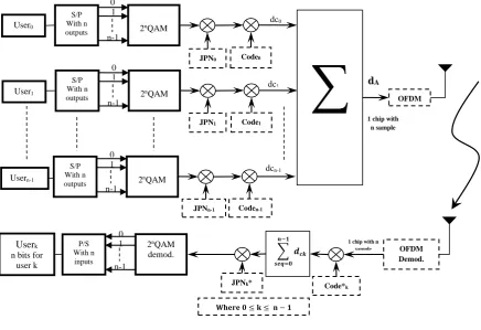
CDMA System
Communication systems today are growing rapidly then the need for high speed or high bit rate with limited bandwidth or limited frequency for that .The multiple inputs multiple outputs (MIMO) system can help with the limitation of band- width frequency (transmitted many users with same frequency) like Time Division Multiplexing Access (TDMA) and Code Division Multiplexing Access (CDMA) or Multi Carrier Code Division Multiplexing Access (MC-CDMA) like Orthogonal Frequency Division Multiplexing companies with CDMA (OFDM-CDMA) .This paper introduce a proposed systems those will use the complex number as data (consolation data like n-QPSK and n-QAM where n is power of 2) with many transforms like Fast Fourier Transform Matrix (FFTm) ,Safe Transform (𝕊𝒏𝒙𝒏), Slantlet, Wavelet, Jwavelet , Hadamard and so on. Instead of the old systems, the Mixed Transform is applied in the CDMA system especially in the Direct Sequence DS-CDMA (JCDMA) with security that uses the complex number like pseudo noise (JPN) and also works in binary form, in this way the derivatives of equations are included in the researcher work papers. The results show that we can increase the data bitrates with gain 1-3 dB from classic CDMA and from OFDM about 14dB when using MC-JCDMA using n-QAM and with normalize the two systems [2], for more see [2].
It is clear that using many orthogonal codes can achieve many advantages like security, anti-interference, and synchronization, which will be discussed later in another paper.
Fig 18: Power spectrum for systems
7.
Conclusion and Future Works
This paper introduce a brand new method for making the mixed transformation has better performance in DSP, for example if we need frequency domain and time domain we can use FFT matrix then tensor with Wavelet instead of using the old way that multiply the signal with FFT matrix then with Wavelet, that make the transform matrix as a tree with branches have leaves companied properties for two or more transform, the future work will study well the philosophy of this method in colored images processing by taking many transforms mixed together, the result in this paper may be not so good or clear but it is acceptable as a study of mixed transform by tensor in the communication applications especially in CDMA, it can generate many of orthogonal Codes, in this field the Code Hopping (CH) (or Phase Hopping ) can be in reality soon for increasing the security on CDMA system or LTE-A.
Frequency
Power Signal
DS-CDMA
JCDMA Noise level
fc
[image:7.595.53.294.500.711.2]Volume 81– No.19, November 2013
8.
REFERENCES
[1] Saifuldeen Abdulameer Mohammed, “A Propose for a Quadrature – Phase as Full Orthogonal Matrix Transform Compared with FFT Matrix Multiplication and Applied in OFDM System (Safe Transform the Fourier Twins)”,Doi :10.7321/jscse. Vol. 2, No.6.5, Jun pp : 56 – 72
[2] Saifuldeen Abdulameer Mohammed, “Proposed System
to Increase the Bits rat for User in the Chip packet using Complex number in Code Division Multiplexing Access and Pseudo Noise (JCDMA and JPN)”, Published in the proceeding of the Second Scientific Conference of Electrical Engineering University of Technology 4-5 April 2011 CE13 pp 200-211.
[3] Bourbaki, Nicolas (1989), Elements of mathematics,
Algebra I, Springer-Verlag, ISBN 3-540-64243-9.
[4] Karen Lees, “Image Compression using Wavelets”,
thesis, 2002, www.ivsl.org.
[5] P.M.K. Prasad ,Prabhakar Telagarapu and G. Uma
Madhuri, “Image Compression using Orthogonal Wavelets Viewed from Peak Signal to Noise Ratio and Computation Time”, International Journal of Computer Applications (0975 – 888)Volume 47– No.4, June 2012,
www.ivsl.org..
[6] Catherine Bénéteau and Patrick J. Van Fleet, “Wavelets
and Image Compression”, 2009.Tavel, P. 2007 Modeling and Simulation Design. AK Peters Ltd.
[7] Nagamani .K and A G Ananth, “Evaluation of SPIHT Compression Scheme for Satellite Imageries Based on Statistical Parameters”, International Journal of Soft Computing and Engineering (IJSCE) ISSN: 2231-2307, Volume-2, Issue-2, May 2012, www.ivsl.org.
[8] H.B.Kekre, Sudeep D. Thepade, Tanuja K. Sarode and Vashali Suryawanshi, “Image Retrieval using Texture Features extracted from GLCM, LBG and KPE”,
International Journal of Computer Theory and
Engineering, Vol. 2, No. 5, October, 2010, www.ivsl.org.
[9] Nik Shahidah Afifi Md. Taujuddin, Nur Adibah Binti
Lockman “Image Compression using Wavelet
Algorithm”, [email protected],
[email protected], International Seminar on the Application of Science & Mathematics 2011.
[10]Sudhakar Radhakrishnan and Jayaraman Subramaniam,
[image:8.595.70.507.367.666.2]“Novel Image Compression Using Multi-wavelets with SPECK Algorithm”, the International Arab Journal of Information Technology, Vol. 5, No. 1, January 2008.
Fig 19: JCDMA 𝐖𝐡𝐞𝐫𝐞 𝟎 ≤ 𝐤 ≤ 𝐧 − 𝟏
User0
JPN0 Code0 dc0
∑
dAOFDM
1 chip with n
sample OFDM
Demod. JPNk* Code*
k
∑ 𝒅𝒄𝒌
𝒏−𝟏
𝒔𝒆𝒒=𝟎 S/P
With n
outputs 2
nQAM
1
n-1
User1
JPN1 Code1 dc1 S/P
With n
outputs 2
nQAM
0 1
n-1
Usern-1
JPNn-1 Coden-1 dcn-1 S/P
With n
outputs 2nQAM
0 1
n-1
Userk
n bits for user k
P/S With n inputs
2nQAM
demod. 1
n-1 0
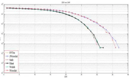
Fig 20: Performance of the all proposed systems and codes
(SNR and BER with number of 4-bits /user/chip in the selective fading channel with 100 Doppler).
a-Safe matrix b-Walsh matrix
d-Slantlet matrix
c-FFT matrix
e-Wavelet and Jwavelet matrix