Practical Guidelines for Learning Bayesian Networks from Small Data Sets

http://dx.doi.org/10.4236/oalib.1100481

How to cite this paper: Bookholt, F.D., Stuurman, P. and Hanea, A.M. (2014) Practical Guidelines for Learning Bayesian Networks from Small Data Sets. Open Access Library Journal, 1: e481. http://dx.doi.org/10.4236/oalib.1100481

Practical Guidelines for Learning Bayesian

Networks from Small Data Sets

F. D. Bookholt, P. Stuurman, A. M. Hanea

Delft Institute of Applied Mathematics, Delft University of Technology, Delft, Netherlands Email: [email protected], [email protected], [email protected]

Received 21 April 2014; revised 26 May 2014; accepted 12 June 2014

Copyright © 2014 by authors and OALib.

This work is licensed under the Creative Commons Attribution International License (CC BY). http://creativecommons.org/licenses/by/4.0/

Abstract

Model learning is the process of extracting, analysing and synthesising information from data sets. Graphical models are a suitable framework for probabilistic modelling. A Bayesian Network (BN) is a probabilistic graphical model, which represents joint distributions in an intuitive and efficient way. It encodes the probability density (or mass) function of a set of variables by specifying a number of conditional independence statements in the form of a directed acyclic graph. Specifying the structure of the model is one of the most important design choices in graphical modelling. Notwithstanding their potential, there are several limitations to learning BNs from small data sets. In this paper, we introduce a set of practical guidelines a modeller can use to deal with these limi-tations. The main goal of the guidelines is to increase awareness of the underlying assumptions and the tacit implications of several learning techniques. Unsurprisingly, one of the authors’ find-ings is that learning BNs from small data sets is a complex and challenging task, yet potentially very rewarding. The paper also draws attention to the amount of subjective input needed from the modeller and the necessity to tailor solutions on the particularity of the application.

Keywords

Hybrid Bayesian Networks, Test for Conditional Independence PC Algorithm, Modeling Choices, Small Data Sets, Structure Learning

Subject Areas: Mathematical Statistics, Network Modeling and Simulation

1. Introduction

1.1. Goal of the Paper

2

(BN) is a probabilistic graphical model that provides an elegant way of expressing the joint distribution of a number of interrelated variables. BNs have been successfully used to represent uncertain knowledge, in a con-sistent probabilistic manner, in a variety of fields. When joint data is available, the structure of the BN may be inferred/learned from data.

The goal of this paper is to propose a sequential overview of the steps a modeller has to take when learning such a structure from data. Since enough literature is available for situations that concern sufficiently big data sets or data that clearly follow some parametric distribution (Gaussian, exponential, etc.), the discussion here concentrates on the challenges encountered when working with small and/or incomplete data sets collected in real life applications. The learning process is divided into sequential steps that tackle possible problems that might be encountered. The guidelines go through the following topics: data preparation, algorithms, testing con-ditional independence, data modelling and division in sub-networks, node ordering, directing arcs and learning parameters from little data.

After introducing the guidelines, we use them to learn a network from a real life data set from a medical study on diabetes. Conclusions about factors that influence the presence of the disease (diabetes) are drawn based on the learned network.

1.2. The Power of BNs

A direct relationship between random variables is modelled in a BN as a directed arc from one corresponding node to another. Indirect effects are modelled as directed paths in the graph. In most applications directed arcs represent direct causal influences1. Before jumping to definitions, two examples of problems one can address are presented to get an idea of the power of BN-modelling.

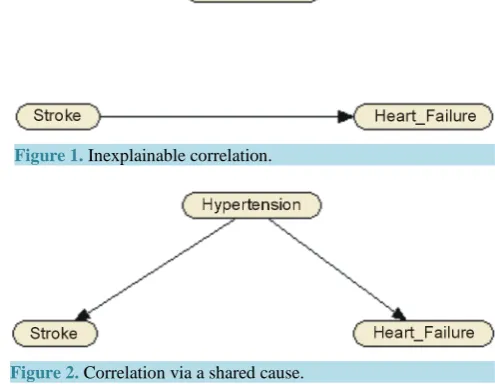
[image:2.595.186.434.512.704.2]

The first problem arises in research where too few factors are taken into account. For instance one may vary some factor A and measure the effects on B whilst keeping all other factors unchanged. Finding a correlation between A and B will often lead a researcher to drawing the general conclusion that A must be causing B. Note that the direction of the causal flow is predefined by the design of the experiment and that other influences are not taken into account. However, one knows that correlations can arise from a shared causal influence which is not taken into account. Consider, for example, Figure 1 and Figure 2. In the former, not taking hypertension into account, one concludes that a patient who suffered a stroke will therefore have an increased chance of heart failure in the future. In the latter, also knowing whether a patient suffers from hypertension, strokes and heart failure become conditionally independent, i.e. the correlation vanishes given the state of a patient’s hypertension. The causal flow then passes through the shared cause and one finds a better representation of the inter variable dependence structure. One sees that the direction of the causal flow can be misinterpreted by the construction of the experiment.

Figure 1. Inexplainable correlation.

Figure 2. Correlation via a shared cause.

3

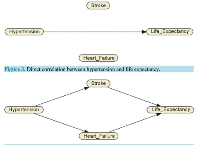
The second type of problem can arise when a correlation found between two factors A and B is an indirect causal effect. Consider the example in Figure 3 and Figure 4. In the former, persistent hypertension is shown to shorten life expectancy. However in the latter, if one takes the patient’s history of strokes and heart problems into account, one sees that the causal effect is indirect. If one knows that a patient has not had a stroke or any heart problems, the correlation between blood pressure and life expectancy ceases to exist. The wrongly drawn conclusion that hypertension is a direct cause of decrease of life expectation can lead to curing the symptoms rather than the cause.

These examples give an impression of the increased insight into the dependence of variables leading to a bet-ter understanding of the nature of causal relations.

1.3. Definitions

A BN is a probabilistic graphical model that represents a set of random variables and their conditional indepen-dences using a directed acyclic graph (DAG). This means that the nodes in the network are connected by di-rected edges in such a way that there are no cycles, thus avoiding causal “chicken and egg” reasoning. The set of nodes (or vertices) is called V and the set of directed edges is called E. Node v∈V is associated with random variable X_v on a sample space Ω_{X v}, either continuous or discrete, with some probability density functions

( )

X_v v

f x assigning a probability to each realisation x_v∈ Ω_Xv. Thanks to the acyclicity, one can order (and number) the nodes in the network such that every edge

(

v w,

)

∈E from node v∈V to node w V∈ satisfies

<

v w.

For a node v∈V , this ordering induces the natural notion of its parents Π

( )

v and children C v

( )

con-sisting of the set of nodes having an edge towards v and the set of nodes that v has edges towards. One may call a node with no parental nodes a source node. The set of ancestors A v

( )

consists of Π

( )

v and their parents recursively. Likewise, the set of descendants D v

( )

consists of C v

( )

and all their children recursively.

A connection via an edge from node v to node w typically indicates a suspected direct causal relationship

[image:3.595.151.476.473.711.2]

from v to w. In other words, v causes or influences w directly. An indirect influence is represented by a directed path between two nodes via other nodes in the network. It is important to state that only the absence of a path between two nodes v and w implies independence of their corresponding variables. Nodes that are connected to each other by a, not necessarily directed, path need not be dependent. Once a network is agreed upon and the modeller finds the parameters for the conditional distributions of each node given its parents, the nodes with a path between them can still be rendered independent. However, the absence of a path between two nodes implies (conditional) independence and it is therefore a much stronger statement.

[image:3.595.159.471.598.703.2]

Figure 3. Direct correlation between hypertension and life expectancy.

4

A BN must satisfy the condition2

(

1

) (

1

)

(

( )

)

=1

, , , , = ,

n

n n i i

i

P_ X  X = x  x _=

∏

P X x Π i

where P X

(

_i =x_i Π

( )

i

)

=P X

(

_i= x_i

)

if Π

( )

i =∅. This property entails the conditional independence of a node from all its ancestors given its parents and it is known as the local Markov property:

Definition 1.1. The Local Markov Property: Let v∈V be a node, than for all v:

\ ( )| ( ) .

v V D v v

X ⊥⊥X X_Π ∀ ∈v V

One can express this property in a useful way by inferring

( )

(

_v = _{v i}= _i,

)

=

(

_v = _{v i} = _i,

( )

)

P X x X x i∉D v P X x X x i∈ Π v

For more theoretical notions concerning BNs, the reader is referred to [1]. It is especially the concept of

d-separation that can be useful in thoroughly understanding causal inference in BNs. For a broader view on causal reasoning [2] is recommended.

Perhaps one of the most important features of BNs is that they permit diagnostic and predictive (e.g., bidirec-tional) inference in the event that only subsets of variables of interest may be observed.

1.4. Types of BNs

Discrete: As the name suggests, in discrete BNs one assumes that the nodes represent discrete random variables. A model is fully specified by the marginal distributions of all source nodes and the conditional probability tables for child nodes. No further assumptions about the distributions are necessary. Modelling discrete BNs might be inflexible at times, e.g. when a new parent-node is added, one must re-determine the conditional distributions of all its children.

Continuous: Perhaps the most popular way of dealing with continuous variables is to discretise them.

Natu-rally, after discretising continuous data, one ends up with a discrete BN. Nevertheless the size of the conditional probability tables will explode if a good approximation of the continuous variables is kept via a fine discretisa-tion.

Often, when dealing with continuous BNs, joint normality is assumed and they are called Gaussian or normal BNs. This assumption should be tested beforehand3. For more information on the testing of multivariate normal-ity, see for example [3]. The influence of a parent on a child is viewed as a regression coefficient and each node is regressed on the set of its parents. A Gaussian BN model is fully specified by the means, conditional variances and the regression coefficients of all variables. However, models for other distributions such as mixtures of ex-ponential distributions do exist and they are described in [4]. We will call these models Continuous parametric BNs.

In Continuous non-parametric BNs, nodes can be associated with arbitrary continuous invertible distributions and arcs with conditional rank correlations. The rank correlations are realised by copulae [5] as described in [6]. Any copula can be used but there are great advantages in using the Gaussian copula. To test for Gaussian copula, one can use a statistical test based on the determinant of the correlation matrix [6]. Note that no joint distribution of the variables is assumed. A model is fully specified by the univariate marginal distributions and the number of one parameter copulae parametrised by the rank correlations r.

Hybrid: Hybrid BNs have a mixture of continuous and discrete nodes. In Parametric Hybrid BNs the nodes

have some pre-defined parametric distribution. Learning algorithms are, for example, available for mixed dis-crete-continuous networks where the parents (and not the children) of Gaussian variables may be discrete.

In hybrid non-parametric BNs, the nodes can be associated with arbitrary discrete or continuous invertible distributions and arcs with conditional rank correlations. Again, the reader is referred to [6] for details.

1.5. Learning BNs from Data

Structure learning is a difficult task due to its computational complexity (NP-hard) and memory intensiveness. Structure learning algorithms can be roughly divided into two classes. Constraint based algorithms test conditional

5

independencies sequentially to draw conclusions about the dependence structure whilst Score based algorithms

use heuristics to construct a BN and validate the result with some score function, of which many have been de-veloped. The process ends when the score of sequential BN’s is no longer improving. Examples are the Markov Chain Monte Carlo (MCMC) BN algorithm [7] and the K2 algorithm [8]. The focus of this paper is on the con-straint based algorithms, and they will be further discussed in Step 2 of our guidelines.

2. Guidelines for Learning BNs from Sparse Data

We will now propose guidelines for modellers to use in order to better understand the structure learning process when learning BNs from small data sets. Many BN learning algorithms exist, and most of them are data hungry,

i.e. the number of data points needed to reach a desirable level of statistical significance grows exponentially with the number of observed nodes. The guidelines segment the different steps of the process and discusse the limitations of small data sets for each step. The process depends to a great extent on the modellers’ input and providing more insight into the options and their implications will help a modeller make more justified choices.

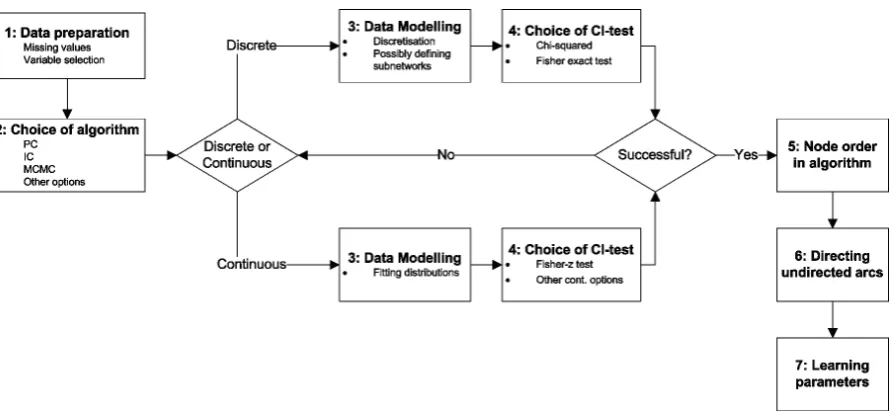
A graphical overview of the steps can be seen in Figure 5. The boxes indicate the seven different steps that are proposed in the structure learning process. The diamond-shaped boxes indicate the decisions that the model-ler has to take. In our experience, the CI-test is the most critical step in becoming intractable. However, using other CI-tests often leads to having to redo the data modelling. This is why after the choice of CI-test, the mod-eller is presented with a possible feedback loop to start again with the data modelling. In the rest of this chapter, each step will be discussed separately.

2.1. Step 1: Data Preparation

[image:5.595.94.542.479.687.2]

In many practical applications, it is impossible to obtain large data sets due to budgetary constraints, time or population size. Furthermore, the data sets will often contain missing values due to, for instance, improper mea-surements or non respondence in a survey. For many BN structure learning algorithms, one needs a fully ob-served data set, so one must deal with these problems. One approach could be to leave out respondents with many missing values, as well as variables with the same problem and to fill the remaining missing values with the mean, median, mode or a sample from the empirical distribution. For specific cases and other methods one can, for example, read [9]. Furthermore, at this stage the modeller must choose which variables will be taken in-to account in the structure learning. One would preferably like in-to include all variables, but this would lead in-to an increase in computational time for the structure learning. Variables that are not of great influence on the main variables of interest can be left out at this stage using light sensitivity analysis [10] or other techniques.

6

2.2. Step 2: Choice of Structure Learning Algorithm

In the category of constraint-based algorithms, the test for conditional independence is often implemented in an oracle or subroutine fashion. The modeler can choose from a variety of different tests discussed in Step 4. Two main categories within the family of constraint-based algorithms are the algorithms that initiate with an empty graph and add arcs and the algorithms that start with a saturated graph and remove arcs.

In the first group, one of the best known algorithms is Inductive Causation (IC). The graph starts with all nodes and no edges. It then connects nodes a and b by an edge if no set S_ab can be found such that

| ab

a⊥⊥b S . Edges are directed using the reasoning of v-structures [11]. Other algorithms that start with an empty graph include the algorithm described in [12] and the SLA-Π algorithm described in [13].

In the second category, the best known is the PC algorithm [11]. It starts with a saturated graph and removes an edge a to b if a set S_ab of neighbours is found such that a⊥⊥b S| ab.

2.3. Step 3: Data Modelling

In order to avoid the problems arising from the increasingly sparse conditional probability tables when using discrete data, one might prefer to model the data as a realisation from some parametric distribution. Especially when fitting normal or exponential distributions, learning algorithms are very efficient. As mentioned above ex-tensions to hybrid parametric BNs exist too.

However, in many practical applications, the nodes do not seem to follow joint normal or exponential distri-butions, so one always has to test this assumption first. Non-parametric continuous or hybrid BNs are a good op-tion if parametric data modelling fails. However, in this case one has to test for the copulae assumpop-tion.

When this fails too, the option of discretising is left, introducing a modelling error as well. The question that arises is how to minimise this error. In practice, a straightforward equal width or equal frequency discretisation will not work since the number of bins must be kept as low as possible in order for the CI-tests to be tractable without losing too much information on the dependence between variables.

An elaborate summary of the available methods is given in [14]. It is particularly useful to minimise the “cor-relation wise error” one introduces by discretisation, because cor“cor-relations are a direct result of the dependence structure. One hopes the dependence structure of the data will be preserved after discretisation.

Even when trying to keep the number of bins per node as small as possible, it is often not possible to learn a complex structure because one might end up with very large conditional probability tables, especially in the case of dense structures. In these circumstances one cannot avoid to split the network into several sub-networks and then learning the structure for each sub-network separately. One can, for instance, define sub-networks by clus-tering groups of nodes with high inter-variable correlations. In this case, connecting the sub-graphs afterwards is a challenge and, to our knowledge, no standard methods to do so exist.

2.4. Step 4: Choice of CI-Test

All constraint-based structure learning algorithms are in some way built around the concept of sequential condi-tional independence tests (CI-tests) so that one can decide whether to remove or add arcs. Many choices are available, depending on the size and nature of the data set. Some of the options are discussed here and differ-ences are distinguished between tests for continuous and discrete data.

2.4.1. Tests on Discrete Data

An obvious choice for a conditional independence test on discrete data is a χ2-type test, as suggested in [15]. Their test statistics converge towards the χ2-distribution with a specific number of degrees of freedom. A modeller has to be careful when using this type of tests when dealing with a small number of data points relative to the number of nodes since this will result in increasingly “bad” convergence which renders the CI-test insig-nificant.

Under the assumption of independence between random variables X and Y, discretised in n_X and n_Y states, the test for independence works as follows. One considers a frequency table in which each cell corresponds to some realisation

(

x y_i, _j

)

that has an observed frequency of O_ij and an expected frequency defined as

= j i

ij

O O E

N

+ ⋅ +

7

Pearson χ2 _{test statistic is now given by}

(

)

2 2

=1 =1

( ) =

n m

ij ij

i j ij

O E X y

E −

∑∑

which converges to the χ2_{-distribution with}

(

₁

) (

₁

)

X Y

n − ⋅ n − degrees of freedom as the number of data points grows. The conditional version of this independence test is obtained by creating this test statistic for every different realisation of a conditioning set of k nodes

{

S₁,,S_k

}

. Here S_i∉

{

X Y,

}

for i= 1,,k and each

i

S is discretised in

Si

n states. Finally, a summation of these values yields the desired conditional CI-test. This CI-test statistic tends to the χ2_{-distribution with}

(

) (

)

=1

1 1

k

X Y _Si

i

n − ⋅ n − ⋅

∏

n (1)

degrees of freedom as N tends to ∞. Other types of χ2-type tests exist, like the Likelihood ratio test.

Agresti points out in [15] that for sparse frequency tables the Pearson χ2-test for conditional independence works better than the Likelihood ratio test. However, the frequency tables must have values bigger than 5 and can have some values as low as 1 if the rest of the table is not very skewed in order for _X2 _{to converge. In}

many practical applications, especially whenever one works with a fine discretisation, frequency tables become increasingly large and the frequency counts can easily drop to values below these lower bounds. Furthermore, checking these conditions on the frequency counts can be computationally expensive and in many implementa-tions of this test, actually a bound on the ratio between degrees of freedom and number of data points is used. This is, in fact, a bound on the average frequency count, not the minimum.

All these facts make us consider another class of conditional independence tests: the exact tests (i.e. not con-verging to some distribution). A well known example is the Fisher exact test4 described in [15]. The p-value for a 2 × 2 frequency table is given by

1 2 11 21 1 = . O O O O p O O + + ++ +               

However, testing for X ⊥⊥Y S| results in k frequency tables of size n × m. This problem causes computa-tional complexity as the number of possible tables given the row and column sums get much bigger. To calcu-late the p-value for a given table, one must calculate the probability of all possible tables and sum all probabili-ties smaller than the probability of the observed table. A mathematical background to the method is provided in [16]. In [17] an n × m generalisation of Fisher’s exact test is implemented. The test uses an exact calculation for 2 × 2, 2 × 3, 3 × 3 and 2 × 4 tables, and does Monte Carlo simulations for bigger tables.

The drawback of this method is that it depends on Monte Carlo simulations for every CI-test. Especially when a model consists of many interconnected nodes, the number of CI-tests to be evaluated by the structure learning algorithm becomes exponentially big. The option to divide the nodes into sub-networks has already been dis-cussed in Step 3, data modelling.

2.4.2. Tests on Continuous Data

A test on continuous data that requires the data to have a normal copula is the CI-test that is based on the Fish-er-z transform. Note that multivariate normality implies the normal copula, but the converse fails to be true.

Suppose

(

X Y,

)

has a bivariate distribution that has a normal copula with a Pearson product moment or a Spearman rank correlation coefficient ρ_{X Y,} and one has a data set of size N with empirical correlation coeffi-cient ρˆ_{X Y,} , then the Fisher-z transform is defined as:

,

, ˆ 1 1

:= ln .

ˆ 2 1 X Y X Y z ρ ρ  +     ₋   

Note that z is approximately normally distributed i.e. 

(

µ σ

, 2

)

with

4

8

,

, 1

1 1

= ln and = .

2 1 3

X Y

X Y N

ρ µ σ ρ  +     ₋  ₋  

Under the assumption of Gaussian copula, one knows the partial correlation coefficient ρ_{X Y S, ;} = 0 is equiv-alent to X ⊥⊥Y S| . One can then use the empirical partial correlation coefficient ρ_{X Y S, ;} to test for (condi-tional) independence. Use Fisher’s z-transform of the empirical partial correlation and introduce the statistical test:

(

)

(

)

0 , ;

1 , ;

5 ˆ

: = 0 |

ˆ

: 0 |

= 0.05 . X Y S

X Y S

H X Y S

H X Y S

ρ ρ α ⇔ ⊥⊥   _{≠ ⇔ ⊥⊥}   

For this test, one has the statistic

(

)

( )

, | = ˆ , ; 3 ~ 0,1 ,

X Y S X Y S

P z ρ ⋅ N− ≥ S − 

and one rejects H₀ if

1

, | > 1 ,

2

X Y S

P Φ− _ −α_

 

where Φ−1 is the inverse standard normal density function. Here S is the number of nodes in the condition-ing set. For further background information on this test, the reader is referred to [18].

In an unpublished study by M. Sneller at Delft University of Technology the kernal-based Conditional Inde-pendence (KCI) Test is used for modelling the same data set. The reader is referred to [19] for the theoretical background to this method.

2.5. Step 5: Node Order in the Algorithm

Structure learning algorithms can or cannot require the modeller to feed the nodes in a specific order. Algo-rithms that do so, often assume the nodes to be ordered descendingly in terms of the parent-child relationships. However, a modeller does not know these relationships beforehand and must therefore base the order on some heuristic. With this, the modeller pre-defines the direction of the flow of causal information in the resulting network and reduces the number of possible networks dramatically.

Other algorithms do not require the nodes to be fed in an order that contains information about the causal structure of the data. However, the resulting network produced by the algorithm does depend on the node order-ing regardorder-ing the presence of arcs as well as their directionality. Among these is the PC algorithm. The reason for this phenomena is that, for example, the PC algorithm removes arcs after a positive CI-test, therefore altering the network and the possible CI-tests that will be performed further on in the process.

There is, to our knowledge, no simple rule for a modeller to make the best choice between these networks, neither does one have the ability to learn the structure of a BN for every permutation of the nodes since this is highly time-consuming. One remark can be made to assist the modeller in making a justified choice. We propose that a modeller learns a network for a couple of radically different permutations of the nodes and then chooses the network with the highest number of arcs. It has already been mentioned that the absence of an arc is a state-ment about independence and that it is therefore much stronger than the presence of an arc since this relation can still be rendered significantly independent when one finally learns the conditional probability densities of the nodes.

Furthermore, a modeller could call in help from an expert in the field of the relevant data set to give a judge-ment on which network is the most intuitive model for the real life situation. One can even reverse the direction of the arcs whenever the chosen direction makes no sense in practice as long as it does not violate the acyclicity in the network.

2.6. Step 6: Directing Undirected Arcs

Many structure learning algorithms produce a Partially Directed Acyclic Graph (PDAG) or randomly choose the

9

unfound directions. In general, not all arcs can be directed on the basis of the data and all possible DAGs for choices of directionality of undirected arcs belong to the same equivalence class. The choice of direction of the undirected arcs will therefore not dramatically change the dependence structure. Some further background in-formation on DAG equivalence classes can be found in [20] and [21].

The modeller now has to direct these arcs by hand. In so doing, one can take two considerations into account. The first and most important one is common sense, preferably based on expert judgement. The second is driven by the underlying data. It is not preferable, in a small data set, for a node to have many parents because of the rapid growth of the number of cells in the conditional probability table. If a node already has over three parents and directing the arc away from the node does not conflict with common sense, then it is the preferable choice.

2.7. Step 7: Learning Parameters

Finally, a modeller has to specify the parameters for the final network. For discrete nodes, this means calculating the values in the conditional probability tables. For continuous nodes, this entails specifying the parameters of the assumed distribution given its parents. Many structure learning software packages have subroutines to do this. However, one must be careful, especially when learning parameters for discrete frequency tables with very low frequency counts since the statistical significance of the obtained conditional probabilities can be very low.

3. A Real Life Case from a Medical Data Set

3.1. The Medical Data Set

In this chapter, we learn the structure for a BN following the recommended steps presented in the flowchart given in Figure 5. The data set is from a medical survey obtained from a group of around 250 patients in the Netherlands. The data consists of a total of 32 continuous and discrete variables, most of which are highly skewed. Among the variables are diabetes-related variables, blood pressures and blood sugar concentrations, as well as other factors like diet, age, sex, weight, etcetera. We are particularly interested in the node “dmbekend”, which states whether a patient is diagnosed with diabetes mellitus type 2. Using the BN we try to find a set of risk factors for this disease. The original data is depicted in Figure 6.

The missing value analysis of Step 1 is done according to our recommendations. In Step 2 we chose the PC algorithm and wrote a recommendation for other researchers to try other algorithms on this data set. The loop of data modelling in Step 3 in combination with different CI-test in Step 4 proved to be more tedious and so we shall elaborate on this topic in the following chapter.

3.2. Data Modelling and CI-Test

In our research, the loop of Step 4 and Step 5 is walked through two times before we arrived at a fruitful result.

3.2.1. First Attempt: Custom Discretisation, Subnetworks Combined with χ2-Type and Fisher

Exact Test

We first tried to discretise the data and use a χ2-type tests. The prevailing problem is the increasing number of degrees of freedom in the conditional probability tables. We therefore refer back to Equation (1). To cope with this problem, we use a custom discretisation to reduce the number of states per variable to a maximum of 5 and a division into subnetworks to reduce the number of nodes per subnetwork to 8.

The discretisation is made by minimising the correlation difference in the correlation matrix of the original data and the that of the discretisation. We used MATLAB to iteratively find the optimal discretisation depicted in Figure 6. In order to check when we have reached a desirable level in the reduction of the correlation wise error, we can calculate the critical value of significance for correlation coefficients. Ramsey states is [22] that the critical value for Spearman correlation coefficients for a data set of n = 100 data points with α = 0.05 is 0.16. Naturally, this number tends to get smaller whenever our data set grows. We managed to reduce this error to below 0.1 for every combination of variables. We propose that one can stop fine tuning the discretisation when-ever the maximum correlation-wise error drops to the level of the critical value for correlation coefficients.

[image:10.595.105.531.82.684.2]

10

Figure 6. The data from the medical research in histograms (blue) together with the used discretisation (red) for the 2

[image:11.595.96.536.86.448.2]

11

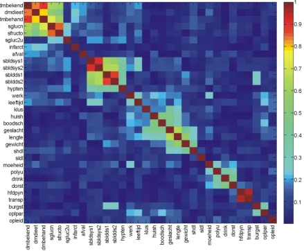
Figure 7. The grouped nodes per subnetworks forming blocks of high correlation.

Despite the efforts made to decrease the number of degrees of freedom, the highly skewed nature of our data set caused most of the χ2-tests to be insignificant and to assume the null hypothesis of dependence ending up with a saturated graph.

We turned to the Fisher exact test, which does not have a lower bound on the frequency counts in the condi-tional probability tables. However, since the condicondi-tional version of this test is based on Monte Carlo techniques and the PC algorithm uses exponentially many CI-test calls, this method turned out to be intractable for our number of variables.

3.2.2. Second Attempt: Gaussian Copula Assumption and Fisher-z CI Test

In our second attempt, we wanted to use the Fisher-z test for conditional independence. The advantage of this method is that partial correlations can be easily calculated in advance to be used in successive CI-tests. The va-lidity of the test is based upon the normal copula assumption. When testing for normal copula, we obtained a positive result, although our data is partly discrete. We decided to use this test to build the structure for our net-work.

Steps 5 to 7 (Determining node order, Directing undirected arcs, Learning parameters) are done according to the recommendation. The result is given in Figure 8.

3.3. Working with the Network

[image:12.595.92.540.83.491.2]

12

Figure 8. The fully directed and quantified network. This figure is created using AgenaRisk (www.agenarisk.com). Note that, although the structure learning with the Fisher-z CI test is done using the complete set of variables, we still group (and colour) the variables using the subnetworks found in the previous step because it seems “natural”.

node “dmbekend”, whether the patient is a known diabetic or not. This allows us to observe changes in all other random variables knowing or observing whether a patient is diagnosed with diabetes. An interesting observation is that the distribution of only six random variables changes upon conditioning. These variables are the diet, the age, the blood sugar values, hypertension and whether the patient has a history of diabetes. All other random va-riables remain unchanged and therefore are of no value for the prediction of diabetes. One could argue that a doctor should not “waste” time on questioning these factors. The converse statement also holds: Conditioning on states of the just mentioned variables changes the distribution of “dmbekend” and conditioning on all other va-riables does not.

We see that a patient with low glucose levels is unlikely to be diabetic despite his or her age. Patients are more often diabetic when the age is between 56 and 70 and glucose levels are very high.

A strange observation is that the probability of a patient being diabetic drops significantly for low glucose le-vels to rise again for large values. This seemingly strange effect can have a medical background or it can be the result of the skewed small data set we are working with. The opinion of an expert will most definitely be helpful in this case.

applica-13

tions. It would be beyond the scope of this article to elaborate further upon this topic.

4. Conclusion

While very promising in applications, learning Bayesian Network structures for small data sets is hard and relies on many modelling choices. Gaining more insight in the modelling process helps a modeller to make more justified choices. The guidelines presented in this paper help to do so. One should refrain from using BN modelling software as a “black box” and keep close track of the assumptions made along the way. In most applications, no standard solutions exist and insight in the different steps of the process is key to obtaining useful and reliable results.

References

[1] Lauritzen, S.L. (1996) Graphical Models. Clarendon Press, Oxford.

[2] Pearl, J. (2000) Causality: Models, Reasoning and Inference. Cambridge University Press, Cambridge.

[3] Krzanowski, W.J. (2000) Principles of Multivariate Analysis: A User’s Perspective. Oxford Statistical Science Series, Oxford University Press, Oxford.

[4] Langseth, H., Nielsen, T., Rumi, R. and Salmeron, A. (2009) Maximum Likelihood Learning of Conditional MTE Dis-tributions. Proceedings of the 10th European Conference, ECSQARU 2009, Verona, 1-3 July 2009.

[5] Joe, H. (1997) Multivariate Models and Dependence Concepts. Chapman & Hall, London. http://dx.doi.org/10.1201/b13150

[6] Hanea, A.M. (2008) Algorithms for Non-Parametric Bayesian Belief Nets. Dissertation, Delft University of Technolo-gy, Delft.

[7] Friedman, N. and Koller, D. (2003) Being Bayesian about Network Structure. A Bayesian Approach to Structure Dis-covery in Bayesian Networks. Machine Learning, 50, 95-125. http://dx.doi.org/10.1023/A:1020249912095

[8] Cooper, G.F. and Herskovits, E. (1993) A Bayesian Method for the Induction of Probabilistic Networks from Data. Technical Report KSL-91-02, Knowledge Systems Laboratory, Medical Computer Science, Stanford University School of Medicine, Stanford.

[9] Little, R.J.A. and Rubin, D.B. (2002) Statistical Analysis with Missing Data. Wiley-Interscience, Hoboken.

[10] Saltelli, A., Chan, K. and Scott, E.M. (2000) Sensitivity Analysis. John Wiley and Sons, Hoboken.

[11] Harris, N. and Drton, M. (2013) PC Algorithm for Nonparanormal Graphical Models. Journal of Machine Learning Research, 14, 3365-3383.

[12] Cheng, J., Bell, D.A. and Lin, W. (1997) An Algorithm for Bayesian Belief Network Construction from Data. School of Information and Software Engineering, University of Ulster at Jordanstown, Jordanstown.

[13] Cheng, J., Greiner, R., Kelly, J., Bell, D. and Liu, W. (2002) Learning Bayesian Networks from Data: An Information- Theory Based Approach. Artificial Intelligence, 137, 43-90. http://dx.doi.org/10.1016/S0004-3702(02)00191-1 [14] Kotsiantis, S. and Kanellopoulos, D. (2006) Discretization Techniques: A Recent Survey. GESTS International

Trans-actions on Computer Science and Engineering, 32, 47-58.

[15] Agresti, A. (1990) Categorical Data Analysis. Wiley Series in Probability and Mathematical Statistics, John Wiley and Sons, Hoboken.

[16] Mehta, C.R. and Patel, N.R. (1983) A Network Algorithm for Performing Fisher’s Exact Test in r c× Contingency Tables. Journal of the American Statistical Association, 78, 427-434.

[17] Cardillo, G. (2010) MyFisher: The Definitive Function for the Fisher’s Exact and Conditional Test for Any R c×

Matrix. http://www.mathworks.com/matlabcentral/fileexchange/26883

[18] Baba, K., Ritei, S. and Masaaki, S. (2004) Partial Correlation and Conditional Correlation as Measures of Conditional Independence. Australian and New Zealand Journal of Statistics, 46, 657-664.

http://dx.doi.org/10.1111/j.1467-842X.2004.00360.x

[19] Zhang, K., Peters, J., Janzing, D. and Schölkopf, B. (2012) Kernel-Based Conditional Independence Test and Applica-tion in Causal Discovery. Max Planck Institute for Intelligent Systems, Tübingen.

[20] Pearl, J. and Verma, T.S. (1990) Equivalence and Synthesis of Causal Models. Proceedings of the 6th Conference on Uncertainty in Artificial Intelligence,Cambridge, 27-29 July, 220-227.

[21] Chickering, D.M. (2002) Learning Equivalence Classes of Bayesian-Network Structures. The Journal of Machine Learning Research, 2, 445-498.