Munich Personal RePEc Archive
Modeling Long-Term Memory Effect in
Stock Prices: A Comparative Analysis
with GPH Test and Daubechies Wavelets
Ozun, Alper and Cifter, Atilla
Marmara University
1 February 2007
Online at
https://mpra.ub.uni-muenchen.de/2481/
Modeling Long-Term Memory Effect in Stock Prices: A
Comparative Analysis with GPH Test and Daubechies
Wavelets
Dr. Alper Ozun a & Atilla Cifter b
a Department of Risk Management, Isbank of Turkey, [email protected]
bDeniz Investment, Dexia Group, and PhD Candidate, Department of Econometrics,
Marmara University, Istanbul, [email protected]
February 2007
Abstract
Long-term memory effect in stock prices might be captured, if any, with alternative models. Though Geweke and Porter-Hudak (1983) test model the long memory with the OLS estimator, a new approach based on wavelets analysis provide WOLS estimator for the memory effect. This article examines the long-term memory of the Istanbul Stock Index with the Daubechies-20, Daubechies-12, the Daubechies-4 and the Haar wavelets and compares the results of the WOLS estimators with that of OLS estimator based on the Geweke and Porter-Hudaktest. While the results of the GPH test imply that the stock returns are memoryless, fractional integration parameters based on the Daubechies wavelets display that there is an explicit long-memory effect in the stock returns. The research results have both methodological and practical crucial conclusions. On the theoretical side, the wavelet based OLS estimator is superior in modeling the behaviours of the stock returns in emerging markets where nonlinearities and high volatility exist due to their chaotic natures. For practical aims, on the other hand, the results show that the Istanbul Stock Exchange is not in the weak-form efficient because the prices have memories that are not reflected in the prices, yet.
Key words: Long-term memory, Wavelets, Stock prices, GPH test
JEL classification: C4, G12, G14
1. Motivation
This article aims to test the long-term partial stationary memory effect in stock prices by wavelet analysis. Finding out the long-term memory parameter in accordance with timescales might be useful for the emerging markets in which high volatility, financial turbulences and chaotic behaviours are observed. By using wavelets in detecting long-term memory effect provides information on memories of the stocks in case f shocks.
Timescaling capital asset pricing model and variance as a risk measure provide an alternative approach for the portfolio theory by giving information on change of risk amount in accordance with hold period and frequency.
or partial stability give financial information that the shock effects might be maintained in long-term and the current prices might depend on the historical price patterns.
Long-term memory indicates the correlation structure of a series at long lags. If a series shows long-term memory, (or the biased random walk), there is persistent temporal dependence even between distant observations. Those time series are characterized by distinct but non-periodic cyclical patterns (Barkoulas and Balum, 2000).
Maheswaran (1990) underlies that the presence of long-term memory in stock returns has important implications for many of the paradigms in financial economics. For example, optimal consumption /savings and portfolio decisions might become extremely sensitive to the investment period if the returns were long-range dependent. There might be also fundamental problems in the pricing of derivatives with martingale methods, since the continuous time stochastic processes most commonly employed are inconsistent with long-term memory.
The presence of long-term memory volatility in stock returns has important implications for pricing contingent claims in emerging markets. High volatility in the capital markets of Turkey as similar to other emerging equity markets creates non-linear behaviours in the stock returns, which might have long-term effect in their time series. Though the markets are expected to be efficient in terms of information flow, the chaotic climate in the emerging stock markets might block the investors to reflect their expectations on the their portfolio decisions or create a long-term effect in the markets especially in case of negative shocks. The negative shocks lead capital markets to affect long-term risk appetite reflected in the stock prices.
The importance of the test results in terms of financial theory, on the other hand, comes from the fact that existence of long-term memory effect in the stock returns implies that the market is not weak form efficient. According to LeRoy (1989), the CAPM and the APT are not valid in the current financial markets because the usual forms of statistical inference do not apply to time series exhibiting such persistence; and tests of efficient markets hypotheses also hang precariously on the presence of long-term memory in the returns. Therefore, this research should also be considered as the examination of the weak-form efficiency in the Istanbul Stock Exchange-30 Index and 100 Index.
As much as we know, this article includes the first empirical research on the long-term memory effect in the share prices at the Turkish capital markets. The long-term memory effect in the Istanbul Stock Exchange-30 Index, and randomly selected ten companies within the ISE-30 Index since 02.01.2002 are examined by using alternative tests, namely Geweke and Porter-Hudak (1983) tests, Hurst Exponent test and wavelet tests (Jensen, 1999; and Tkacz, 2001).
2. Literature Review
Wavelet based integration and causality analysis are applied to the finance and economics by
Jensen (1999, 2000), Jensen and Whitcher (2000) and Whitcher and Jensen (2000) who use the initial works of Wornell and Oppenheim (1992), Tevfik and Kim (1992), McCoy and Walden (1996). Percival and Walden (2000), Tkacz (2001), Gencay, Selcuk and Whitcher (2002) and Vourenmaa (2005) show that wavelet based long-term memory effect model performs better than Geweke and Porter-Hudak (1983) and fractional integration and causality tests. Jin, Elder and Koo (2006) show that wavelet based models solve the abnormal results of the alternative models dealing with long-term memory in the stock prices.
Sowell (1992) suggests an exact maximum-likelihood estimator for long-memory models possessing both short and long-memory parameters, namely the autoregressive, fractionally integrated, moving-average model. However, the assumption of a constant long-memory in the returns might not be reliable in all case. Though Bayraktar et al (2003) argue a solution for the time-varying long-memory by segmenting the data before its prediction, the solution is not always sufficient in that Whitcher and Jensen (2000) argue that the capacity of estimating local behavior by applying a partitioning model to a broad estimating process is not enough when compared with an estimator constructed to model time-varying characteristics. For that reason, in this paper, we use the MODWT-based methodology to estimate long-memory effect.
Wavelets employ Fourier analysis to decompose the variance of time series on different frequencies. The scales contributing the most to the variance of the series are related to those coefficients with the largest variance. Devore, Jawerth, and Popov (1992) state that the capacity of wavelet to localize the time series in multi-scale space causes the computational efficiency of the wavelet representation of an N £ N matrix operator by allowing the N largest elements of the wavelet-represented operator to represent the matrix operator. This feature enables dense matrices to have sparse representation when transformed by wavelets.
Empirical evidences show that though the GPH-estimator based on the ordinary least squares regression of the log-periodogram for frequencies close to zero is consistent under Gaussian distribution, the normality assumption in the distributions are not realistic with financial data which have generally abnormally distributed volatility. In that framework, Jensen (1999)
shows that a wavelet based OLS-estimator is consistent with the real financial dynamics, when the sample variance of the wavelet coefficients is used in the regression.
The wavelets methodology is theoretically well-examined in the works by Schleicher (2002) and Crowley (2005). Usage of wavelets analysis in statistical time series can be followed on
Nason and Von-Sachs (1999). Mathematical concerns on the wavelets are discussed within the work of Hardle et al (1998).
3. GPH Test For OLS Estimator vs. Wavelet Based OLS Estimator
In the methodology part, we discuss the wavelet based OLS estimation and GPH test for detecting the long-term memory effect in the financial time series. Jensen (1999) argues that the wavelets are superior in estimation because of their strength to simultaneously localize a process in time and scale. Wavelets are based on Fourier analysis where any covariance-stationary process xt is expressed as a linear combination of sine and cosine functions in the
frequency domain. However, since few financial time series show smooth rhythmic cycles suggested by sine and cosine functions, an alternative transformation model, namely wavelet transforms where function f(x) on [0,1] interval is expressed in the wavelet domain as
∑
∑
−= ∞
=
= 2 1
0 0 0
c ) (
f
k j
x
f cjkΨ (2jx-k) (1)
On the formula cited from Tkacz (2001),Ψ(x) is mother wavelet, as the mother to all dilations and translations of Ψ in above equation. A mother wavelet can be shown as (Tkacz, 2001)
1, if 0 ≤x < ½
Ψ(x) = 1, if ½ ≤x < 1 (2) 0, otherwise
The functions of Ψjk(x) = Ψ (2jx-k) for j ≥0 and 0 ≤k < 2j are orthogonal, and they create a
basis in the space of all square-integrable functions L2 along the [0,1] interval. j is the dilation
index compressing the function Ψ(x), and k is the translation index shifting the function Ψ(x). Any such basis in L2(R)is a wavelet, and the Equation 2 is the Haar wavelet (Tkacz, 2001).
Among several wavelets models in the literature we use Daubechies model (1988), which has supported wavelets whereby each wavelet represents different degrees of smoothing of the step function, namely the Equation 2. By following Tkacz (2001), we use different Daubechies and the Haar wavelets to verify the robustness of the results to different degrees of smoothing. The Daubechies-20 wavelet is used as the smoothest wavelet, followed by the Daubechies-12 and the Daubechies-4, with the Haar wavelet being the least smooth.
To test the long-term memory effect with wavelet based OLS estimator, we use Jensen (1999)
and Tkacz (2001) technique. The matlab codes used by Tkacz (2001) are restructured for the empirical analysis. The WOLS estimator can be formulized as follow:
Let define xt as a random process,
(1-L)dxt = et (3)
where L is the lag operator, et is i.i.d. normal with zero mean and constant variance σ2, and d
is a differencing parameter. The wavelet OLS estimator of d comes from the smooth decay of long-memory processes. When d=0, the random process xt equals to et and therefore, xt ~
(N(0, σ2), or xt ~ I(0). On the other hand, when d=1, xt follows a unit root process with a zero
If d is noninteger, the random xt process becomes fractionally integrated, namely ARFIMA
process as shown on the Equation 3. Hosking (1981) shows that when 0<d<½ the autocovariance function of the random process declines hyperbolically to zero as a long-memory process. When ½ d<1, the random process takes an infinite variance but still reverts to its trend in the very long run (Tkacz, 2001). On the Table 1, the features of the fractional integration parameter (d) are summarized.
≤
Table 1: Memory Features With Respect to the Fractional Integration Parameter Values
D Variance Shock Duration Stationarity
d =0 Finite Short Memory Stationary 0< d <0.5 Finite Long Memory Stationary 0.5≤ d <1 Infinite Long Memory -Finite
Impact-Reflect
Nonstationary
d=1 Infinite Finite-Not Revert to Its Mean Nonstationary
d >1 Infinite Finite-Not Revert to Its Mean Nonstationary
Source: Tkacz, G. (2001), Estimating the Fractional Order of Integration of Interest Rates Using a Wavelet OLS Estimator, Studies in Nonlinear Dynamics & Econometrics, 5(1): pp. 23.
Tevfik and Kim (1992), McCoy and Walden (1996), Jensen (1999) and Tkacz (2001)
empirically show that for an I(d) process xt with /d/< ½ , the autocovariance function shows
that the wavelet coefficients cjk in Equation 1 are distributed as N (0; σ2 2-2jd). By taking
logarithms, an estimate of d can be reached using ordinary least squares from
ln R( j) = ln σ2 – dln22j (4)
where R j denotes the wavelet coefficient’s variance at scale j (Tkacz, 2001). In that
framework, Tkacz (2001) states that the wavelets are used only in the estimation of the d
consistent with the observed autocovariance function. What’s more, the number of observations for the random process should be a factor of two due to the form of the wavelet expansion 1.
To detect the long-term memory effect in stock returns, Geweke and Porter-Hudak (1983)
test, Hurst Exponent test and wavelets are used. Long-memory was firstly developed by Hurst (1951) and adopted into the econometrics by Granger and Joyeux (1980) and Geweke and Porter-Budak (1983).
The GPH test starts with the spectral density function of xi (Kasman, Kirbas and Turgutlu,
2005):
{
4sin ( /2)}
( ) )2 / ( )
(λ σ2 π 2 λ d u λ
x f
f = − (5)
) (λ
u
f , is the spectral density function of ui at λ frequency. After taking logarithmics and including I(λj), at j ordination, the Equation 5 is reached (Chambers ve Cifter, 2006).
{
I( j)}
In{
2fu(0)/2}
dIn{
4sin2( /2)}
In{
I( j)/ f ( j)}
When λj has low frequency, In
{
fu(λj)/ fu(0)}
becomes inefficient. GPH regression can beformulated as
[
I j]
In[
j]
ujIn (λ ) = β0 +β1 4sin2(λ /2) + (7)
The constant term, β0, is (In
{
σ2fu(0)/2π}
), β1=-d, uj=In{
I(λj)/ fχ(λj)}
as the error term.If lim ( )2/ ( )=0, then asymptotic distribution of is formulized by the Equation 8.
∞
→ g T g T
T dGPH
∧
⎟ ⎠ ⎞ ⎜
⎝ ⎛
−
→
∑
=
∧ n
i i
GPH N d x x
d
1 2
( 6 /
,π (8)
i
x =In
[
4sin2(λj/2)]
. In the GPH test, if , provides statistically acceptable and asymptotic normality.0
<
∧
d dGPH
∧
4. Data
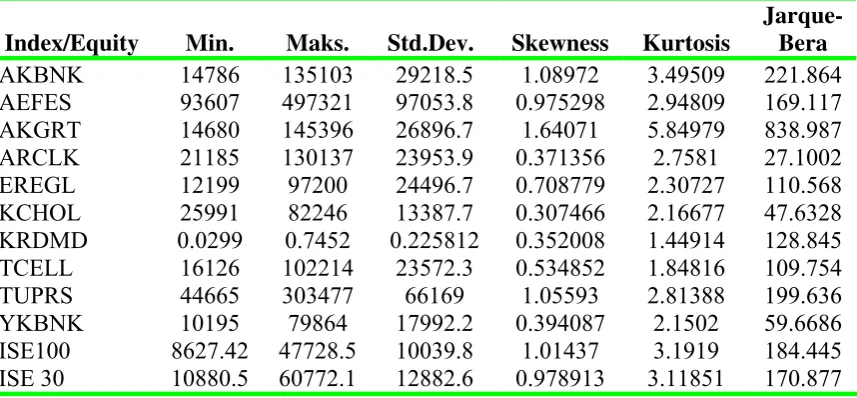
[image:7.595.77.506.498.697.2]The data is obtained from 10 common stocks namely AKBNK, AEFES, AKGRT, ARCLK, EREGL, KCHOL, KRDMD, TCELL, TUPRS and YKBNK, all of which are included in ISE-30 index. These shares have been selected randomly and they represent 33% sample rate (10/30). Further, ISE 100 index has also been considered as an analysis subject. In this sense, the empirical study provides a wide range comprising ISE 30 and ISE 100 indexes along with the randomly selected shares from ISE 30. The volatility of the returns of the selected stocks depending on the size, systematic risk and long-term memory parameter are determined by using wavelet analysis. The statistical features of the selected stocks are available in Table 2. All stocks can be accepted in normal distribution according to Jarque-Bera normality test, and their depressiveness and distortion features are different from those of each other’s.
Table 2: Descriptive Statistics
Index/Equity Min. Maks. Std.Dev. Skewness Kurtosis
Jarque-Bera
AKBNK 14786 135103 29218.5 1.08972 3.49509 221.864 AEFES 93607 497321 97053.8 0.975298 2.94809 169.117 AKGRT 14680 145396 26896.7 1.64071 5.84979 838.987 ARCLK 21185 130137 23953.9 0.371356 2.7581 27.1002 EREGL 12199 97200 24496.7 0.708779 2.30727 110.568 KCHOL 25991 82246 13387.7 0.307466 2.16677 47.6328 KRDMD 0.0299 0.7452 0.225812 0.352008 1.44914 128.845 TCELL 16126 102214 23572.3 0.534852 1.84816 109.754 TUPRS 44665 303477 66169 1.05593 2.81388 199.636 YKBNK 10195 79864 17992.2 0.394087 2.1502 59.6686 ISE100 8627.42 47728.5 10039.8 1.01437 3.1919 184.445 ISE 30 10880.5 60772.1 12882.6 0.978913 3.11851 170.877
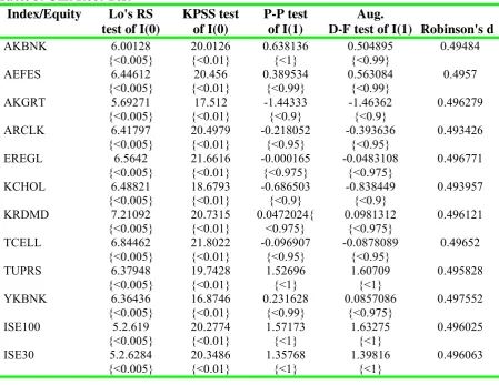
In the Table 3, the stability values of the stocks are given according to Lo's RS test, KPSS test, P-P test, Augmented Dickey Fuller test and Robinson D test. All series are stable to logarithmic difference.
Table 3: Unit Root Test
Index/Equity Lo's RS test of I(0)
KPSS test of I(0)
P-P test of I(1)
Aug.
D-F test of I(1) Robinson's d AKBNK 6.00128 {<0.005} 20.0126 {<0.01} 0.638136 {<1} 0.504895 {<0.99} 0.49484 AEFES 6.44612 {<0.005} 20.456 {<0.01} 0.389534 {<0.99} 0.563084 {<0.99} 0.4957
AKGRT 5.69271
{<0.005} 17.512 {<0.01} -1.44333 {<0.9} -1.46362 {<0.9} 0.496279
ARCLK 6.41797
{<0.005} 20.4979 {<0.01} -0.218052 {<0.95} -0.393636 {<0.95} 0.493426
EREGL 6.5642
{<0.005} 21.6616 {<0.01} -0.000165 {<0.975} -0.0483108 {<0.975} 0.496771
KCHOL 6.48821
{<0.005} 18.6793 {<0.01} -0.686503 {<0.9} -0.838449 {<0.9} 0.493957
KRDMD 7.21092
{<0.005} 20.7315 {<0.01} 0.0472024{ <0.975} 0.0981312 {<0.975} 0.496121
TCELL 6.84462
{<0.005} 21.8022 {<0.01} -0.096907 {<0.95} -0.0878089 {<0.95} 0.49652
TUPRS 6.37948
{<0.005} 19.7428 {<0.01} 1.52696 {<1} 1.60709 {<1} 0.495828
YKBNK 6.36436
{<0.005} 16.8746 {<0.01} 0.231628 {<0.99} 0.0857086 {<0.975} 0.497552
ISE100 5.2.619
{<0.005} 20.2774 {<0.01} 1.57173 {<1} 1.63275 {<1} 0.496025
ISE30 5.2.6284
{<0.005} 20.3486 {<0.01} 1.35768 {<1} 1.39816 {<1} 0.496063
5. Empirical Evidence
In Table 4, there are stability test results according to Geweke and Porter-Hudak method. The long-term memory parameter (d) changes between 0.98138 and 1.08555. The series are not stable and the shock period is infinite (non-returnable in the average of series), since the long term memory parameter is closing to 1, in the long-term. Owing to the long-term memory parameters of KCHOL and KRDMD are smaller than 1, these series are not stable and have long term memory. According to GPH method, it is evidenced that the stocks other than KCHOL and KRDMD are not stable, and no-returning is available in the averages of the series.
Table 4 : Fractional Integration Parameters With Geweke/Porter-Hudak Method *
Index/Equity d T(d) Bias Test: ChiSq(1)
AKBNK 1.07727 14.583 0.273943 {0.601}
AEFES 1.06873 14.468 0.443364 {0.506}
AKGRT 1.08555 14.695 0.00479251 {0.945} ARCLK 1.01197 13.699 0.351684 {0.553}
EREGL 1.07203 14.512 0.500397 {0.479}
[image:8.595.77.495.642.764.2]KRDMD 0.98138 13.285 0.327224 {0.567}
TCELL 1.0949 14.822 0.334297 {0.563}
TUPRS 1.01841 13.787 1.17552 {0.278}
YKBNK 1.08551 14.695 2.52501 {0.112}
ISE 100 1.06538 14.422 0.162058 {0.687} ISE 30 1.07107 14.499 0.150576 {0.698}
* Bandwidth = 90 (= T^0.65)
[image:9.595.73.498.71.166.2]All series are not stable and shock period is infinite according to Fractal Dimension – Hurst Exponent. In other words, the series do not return to their averages. In case of taking the difference of the series, all series are stable and the shock period is permanent (Table 5).
Table 5 : Fractal Dimension – Hurst Exponent
Series Difference Series
Index/Equity
H Standart Dev. (H) R2
H Standart Dev. (H) R2
AKBNK 1.0216 0.002054 0.9948 0.8141 0.006859 0.9915 AEFES 1.0137 0.001837 0.9995 0.8055 0.006702 0.9916 AKGRT 1.0249 0.001866 0.9995 0.8081 0.006830 0.9911 ARCLK 1.0230 0.002052 0.9995 0.8118 0.006781 0.9913 EREGL 1.0208 0.002164 0.9994 0.8113 0.005877 0.9936 KCHOL 1.0271 0.001817 0.9996 0.8246 0.006629 0.9921 KRDMD 1.0078 0.001994 0.9994 0.7706 0.006956 0.9904 TCELL 1.0163 0.001578 0.9996 0.8217 0.006401 0.9925 TUPRS 1.0093 0.002565 0.9991 0.7923 0.006644 0.9917 YKBNK 1.0310 0.002317 0.9993 0.8118 0.003744 0.9970 ISE 100 1.0190 0.001391 0.9997 0.7590 0.005861 0.9928 ISE 30 1.0144 0.001236 0.9998 0.7563 0.005890 0.9927
* Bandwidth = 90 (= T^0.65)
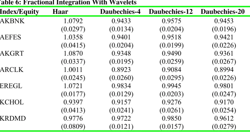
[image:9.595.77.502.541.767.2]The partial stability test results of 10 stocks from ISE-30 according to Daubechies-4, Daubechies-20 and Daubechies-20 wavelet are available in the table 3.16.
Table 6: Fractional Integration With Wavelets
Index/Equity Haar Daubechies-4 Daubechies-12 Daubechies-20
AKBNK 1.0792 (0.0297) 0.9433 (0.0134) 0.9575 (0.0204) 0.9453 (0.0196) AEFES 1.0358 (0.0415) 0.9401 (0.0204) 0.9518 (0.0199) 0.9421 (0.0226) AKGRT 1.0870
(0.0337) 0.9348 (0.0195) 0.9490 (0.0259) 0.9361 (0.0267) ARCLK 1.0011
(0.0245) 0.8923 (0.0260) 0.9084 (0.0295) 0.8994 (0.0226) EREGL 1.0721
(0.0177) 0.9834 (0.0129) 0.9945 (0.0203) 0.9801 (0.0247) KCHOL 0.9397
(0.0413) 0.9157 (0.0241) 0.9276 (0.0261) 0.9170 (0.0254) KRDMD 0.9776
TCELL 1.0316 (0.0372)
0.9726 (0.0119)
0.9825 (0.0200)
0.9570 (0.0368) TUPRS 1.0548
(0.0368)
0.9414 (0.0125)
0.9458 (0.0180)
0.9312 (0.0203) YKBNK 1.0125
(0.0372)
0.9543 (0.0541)
0.9682 (0.0382)
0.9548 (0.0349) ISE 100 1.1104
(0.0279)
0.9544 (0.0102)
0.9678 (0.0196)
0.9531 (0.0237) ISE 30 1.1002
(0.0274)
0.9561 (0.0097)
0.9691 (0.0186)
0.9540 (0.0232)
Note: The values in the paranthesis are standart deviation.
The findings found by using Harr wavelet are in parallel with GPH method. By performing Daubechies 4, 12 and 20 days wavelet analysis, it is found that all series can return to their averages where as they are not stable completely (0.5≤ d <1), and series has finite impact-response weight. Parameter d’s being within the range of 0,89-0,98 and closing of the memory parameter in the long-run show that prediction models based on past period volatility can be effective in the long run for the stocks included in ISE 30.
6. Concluding Remarks
Detecting long-term memory effect in stock prices has fundamental results for both methodological concerns and portfolio management. Efficient market hypothesis states that the information comes into the markets is reflected in the prices immediately, thus the historical time series does not present any clues for the future prices. In other words, the markets are memoryless.
On the other hand, interdisciplinary applications in the literature give opportunity to construct the advanced methodological models for the financial economics. In this paper, wavelets used in the quantum physics are applied for the fractional integration parameter detecting the long-term memory in the stock returns. Due to relatively high volatility and turbulences in the emerging capital markets, wavelets are proper to use in detecting long-term behaviours in the returns by filtering short-term biased movements arising from the asymmetric information flows.
This paper comparatively examines the alternative methods to model the long-term memory effect in the stock returns. The empirical findings show that methodological concerns create crucial differences, which might affect the decisions of the investors. While the results of OLS estimators based on the GPH tests imply that the markets are in the weak-form efficiency, the wavelets based OLS estimators display the fact that the prices have memory stating that analyzing the time series might be still effective in estimating the future behaviours in the returns.
In the long-term memory analysis, despite the long term parameter of GPH and Hust Test is in the level of 1. The d is calculated within the range of 0.89-0,98 according to Daubechies 4,12 and 20-day wavelets. The closing of long-term memory parameter in the long run suggest that prediction models base on the past period volatility can be effective.
the prediction performance. As a result of the study, it is concluded that wavelet method can be applied to develop strategy in the different frequencies (scales) in finance engineering and portfolio management.
References
Barkoulas, J.T. & Baum, C.F., (1996) "Long-term dependence in stock returns," Economics Letters, 53(3) : 253-259.
Bayraktar, E, Poor H.V. and Sircar, K.R., (2003) “Estimating the Fractal Dimension of the S&P 500 Index Using Wavelet Analysis”, Working Paper, Department of Electrical Engineering, Princeton University, 2003.
Cifter, A. and Chambers, N., (2006) “Testing Fractional Integration of Forward Rat Unbiasedness Hypothesis: Evidence from Turk DEX”, Proceeding of the Internatıonal Fınance Symposıum, Marmara University, 2006.
Crowley, P., (2005) "An intuitive guide to wavelets for economists," Research Discussion PapersBank of Finland, 1/2005.
Daubechies, I., (1988) “Ortonormal bases of compactly supported wavelets”,
Communications on Pure and Applied Mathematics, 41: 909-996
Devore, R., Jawerth, B. and Popov, V., “Compression of wavelet decompositions”, American Journal of Mathematics, 114:737-785.
Gencay, R., Seluk, F., Whitcher, B. (2002) “An Introduction to Wavelets and Other Filtering Methods in Finance and Economics”, Academic Press.
Geweke, J., and Porter-Hudak, S. (1983), “The estimation and application of long memory time series models”, Journal of Time Series Analysis, 4: 221–238.
Granger, C.W.J. and Joyeux, R. (1980) “An Introduction to Long Memory Time Series Models and Fractional Differencing”, Journal of Time Series Analysis 1: 15-29.
Hardle,W., Kerkyacharian, G., Picard, D. and Tsybakov, A. (1998) “Wavelets, Approximation, and Statistical Applications”, Springer, New York.
Hosking, J. R., (1981) “Fractional differencing”, Biometrika, 68: 165–176.
Hurst, H. E. (1951) “Long Term Storage of Reservoirs”, Transactions of the American Society of Civil Engineers, 116: 770-799
Jensen, M. J., (1999) “Using wavelets to obtain a consistent ordinary least squares estimator of the long-memory parameter”, Journal of Forecasting, 18: 17–32.
Jensen, M.J. and Whitcher, B. (2000) “Time-Varying Long-Memory in Volatility: Detection and Estimation with Wavelets”, Technical report, University of Missouri and EURANDOM.
Jin, Hyun J., Elder, J., Koo, W.W., (2006) "A reexamination of fractional integrating dynamics in foreign currency markets," International Review of Economics & Finance, 15(1): 120-135
Kasman, A. Kirbas, K.B. and Turgutlu, E. (2005) “Nominal and Real Convergence Between the CEE Countries and the EU: A Fractional Cointegration Analysis", Applied Economics, 37: 2487-2500
LeRoy, S.F. (1989) “Efficient Capital Markets and Martingales”, “Journal of Economic Literature”, 1583-22.
Maheswaran S., (1990), "Predictable Short-Term Variation in Asset Prices: Theory and Evidence," Working Paper, Carlson School of Management, University of Minnesota
McCoy, E. J., and A. T. Walden. (1996). “Wavelet analysis and synthesis of stationary long-memory processes” Journal of Computational and Graphical Statistics, 5: 1–31.
Nason, G.P. and von Sachs, R. (1999) “Wavelets in Time Series Analysis”, Philosophical Transactions of the Royal Society of London, Series A 357, 2511-2526.
Percival, D.B. and Walden, A.T. (2000) “Wavelet Methods for Time Series Analysis”,
Cambridge University Press.
Schleicher, C. (2002) “An Introduction to Wavelets for Economists”, Monetary and Financial Analysis Department, Bank of Canada, Working Paper 2002-3.
Sowell, F. (1990). “The fractional unit root distribution.” Econometrica, 58: 495–505.
Tevfik, A. H., and M. Kim. (1992). “Correlation structure of the discrete wavelet coefficients of fractional Brownian motion.” IEEE Transactions on Information Theory, 38: 904–909.
Tkacz, G., (2001) “Estimating the Fractional Order of Integration of Interest Rates Using a Wavelet OLS Estimator”, Studies in Nonlinear Dynamics&Econometrics, 5 (1).
Vuorenmaa, T. (2004) “A Multiresolution Analysis of Stock Market Volatility Using Wavelet Methodology”, Licentiate Thesis, University of Helsinki.
Whitcher, B. and Jensen, M.J. (2000) “Wavelet Estimation of a Local Long Memory Parameter”, Exploration Geophysics, 31: 94-103.