On Board Near Optimal Flight Trajectory Generation using Deferential Flatness

On-Board Near Optimal Flight Trajectory Generation

using Deferential Flatness

R. Esmaelzadeh

Space Research Institute Tehran, Iran

ABSTRACT

An optimal explicit guidance law that maximizes terminal velocity is developed for a reentry vehicle to a fixed target. The equations of motion are reduced with differential flatness approach and acceleration commands are related to trajectory’s parameters. An optimal trajectory is determined by solving a real-coded genetic algorithm. For online trajectory generation, optimal trajectory is approximated. The approximated trajectory is compared with the pure proportional navigation, and genetic algorithm's solutions. The near optimal terminal velocity solution compares very well with these solutions. The approach robustness is examined by Monte Carlo simulation. Other advantages such as trajectory representation with minimum parameters, applicability to any reentry vehicle configuration and any control scheme, and Time-to-Go independency make this guidance approach more favorable.

Keywords

Reentry, Explicit Guidance, Differential Flatness, Optimal Guidance, Real Genetic Algorithm.

1.

INTRODUCTION

The general solution of the optimal flight of a reentry vehicle (RV) to an arbitrary, but specified, final condition has been of interest for some time. Contensou was the first to consider optimal control and proposed the problem for unconstrained range in terms of flight path angle as the independent variable [1]. Eisler and et al. [2], using neighboring optimal control, devised a sampled-data feedback control method to obtain unconstrained, approximate, maximum-terminal-velocity descent trajectories at a designated target. This maximization has the dual advantage of reducing the time to reach the target as well as maximizing the kinetic energy level.

Generally, the design of guidance algorithms may be defined loosely as the art of finding the correct acceleration commands to move between two given points. Many different techniques have been suggested for the design of guidance algorithms. These range from the earliest algorithms derived using physical insight (e.g., pursuit, proportional navigation (PN) and their variants) to those derived from a systematic application of mathematical techniques. Most current guidance design methods may be classified into two main categories [3]: (1) nominal trajectory-based techniques and (2) on-line trajectory generation, reshaping and prediction schemes. In the first approach, an (optimal) reference trajectory is defined prior to the mission, and during the flight, a controller keeps the vehicle close to the nominal trajectory. The predictive and/or reshaping approaches propagate the future trajectory based on current flight state by means of onboard numerical integration to calculate the control input during the remaining flight.

Explicit guidance methods are good examples of the second category. A review of literature [4] shows that they have

many advantages over other approaches. These methods, which use preset external trajectories, give a huge calculation advantage and can provide a near optimal solution with any desired accuracy. These are applicable to systems that have linear acceleration and aim at constructing guidance algorithms with specified desired dynamics (i.e. solving an inverse problem.). Although some authors [5, 6] have considered the inverse problem as a direct method because of the implicitly parameterized control, it is better that this approach is examined within a different class. In a direct method, the trajectory of the vehicle must be predicted if the initial conditions and the time history of the controls are given, meaning Cauchy task, whereas in an inverse problem, the controls that are compatible with a desired trajectory must be predicted [7]. Inverse methods are of great interest in the context of synthesizing nonlinear autopilots [8-10] and guidance algorithms [11-15]. A survey about the inverse problem approach in optimal trajectory generation, both in Russia and in the United States, can be found in Yakimenko’s paper [5]. In guidance applications, the variable guidance gains are correlated with the shape of the trajectory that will follow and satisfy particular terminal constraints. Although, with an extension of Taranenko [15], Cameron [16], and Page's [17] methods, the use of this approach in guidance algorithm design has been developed by Hough [11] and Yakimenko [5], it still suffers from serious flaws: a relatively large number of optimization parameters (Ops) (Taranenko, 20; Mortazavi [18],‌‌ 12; and Hough, 8) depending on the vehicle's velocity vector, relatively difficult numerical calculations, accuracy dependence on the number of segments used in the approximation, and offline application.

In this paper, the author extends the previous works done on maximizing terminal velocity [19-21]. An explicit guidance law is developed by flatness approach for guiding a hypersonic unthrusted reentry vehicle (RV) to a fixed point on the ground (Eisler’s problem [2]). . The guidance commands are related to geometrical trajectory shape and constraints. The guidance law is based on the normal and side accelerations. At the next step, the guidance law is optimized using real-coded genetic algorithms (RGA). The present paper deals with a new, in some sense, simplified method that provides near optimal spatial trajectories being presented analytically and completely defined by minimum OPs. This method has a number of advantages over methods presented by Taranenko, and Hough. Although guidance law is designed for an RV, it can also be applied to any vehicle at any phase.

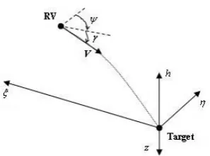
Fig 1: Geometrical definitions.

2.

PROBLEM DEFINITION

Assuming a spherical, nonrotating Earth (this assumption was made for simplicity, but a similar guidance law can be derived based on more precise equations of motion including terms due to earth rotation) and a gravitational field with g/r2, three-dimensional point mass equations of motion for the RV (Fig. 1) can be written as:

                sin -/ sin cos -/ cos cos -/ cos / / d / ) cos ) / -( ( / d / ) -sin ( / d h c 2 v c V t d dh h V t d d V t d d V a t d V r V g a t d m D mg t d V V                    (1)

where V is velocity,  is flight path angle,  is yaw angle,  is range,  is cross-range, h is altitude, t is the time variable, m is RV mass, D is drag force, ahc is horizontal acceleration command, and avc is vertical acceleration command. For the bank-to-turn control configuration (BTT):

m L a m L

avc  cos/ , hc sin/

where  is bank angle..

The guidance problem is to find acceleration commands (or equivalently , and  for BTT), which steer the vehicle to its target, subject to the state equations (1); known initial conditions, V0, 0, 0, 0, 0, and h0; and known final conditions, f, f, and hf (equivalent to a fixed target position). The solution must satisfy the following constraint:

max 2 hc 2 vc

c a a ≤ a

a   (2) The amax can be related to the limitations of angle of attack, dynamic pressure, heat transfer, loading, etc.

3.

COMPUTATIONAL ALGORITHM

3-1-Differential Flatness

Differential flatness was first introduced by Fliess and el al [22] in a differential algebraic context. The important property of flat systems is that a set of variables (equal in number to the number of inputs) can be found such that all states and inputs can be expressed in terms of those outputs and a finite number of their time derivatives without any integration procedure. More precisely, the dynamical system of the general form may be considered as [23]:

)) ( ), ( ( ) ( )) ( ), ( ( ) ( t u t x h t y t u t x f t x   

where x is the n-dimensional state vector, u is the m-dimensional input vector, y is the m-dimensional tracking output vector, f(.) and h(.) are a nonlinear functions. The system is differentially flat if a set of variables z(t)m

can be

found which are differentially independent, called flat outputs, of the form

)) ( ),..., ( ), ( ), ( ( )

(t xt ut ut u() t

z   a

such that )) ( ),..., ( ), ( ( )

(t zt zt z( )t

x x  b

)) ( ),..., ( ), ( ( )

(t zt zt z( 1) t

u _u  b

where  and  are smooth functions, z(a)(t) and z(b)(t) are respectively the a and b order time derivative of z(t).

In situations where explicit trajectory generation is required, differential flatness can be very useful: since the behavior of flat systems is determined by the flat outputs only, the trajectories can be planned in output space and then mapped to the appropriate inputs. Many authors have been used differential flatness approach to reentry problem guidance [23-26]; As it is proved in the study of Neckel and et al [27], the nonlinear model (1) is not flat if h,  and  are considered as flat outputs. To get around this problem, all studies have kept the longitudinal and lateral motions uncoupled. Therefore, only the longitudinal dynamics are inverted using altitude and curvilinear abscissa as flat outputs, the lateral guidance being ensured via a typical roll reversal technique [e.g. 24]. Decoupling has its limitations. For overcoming these limitations, choosing  and  as flat outputs and solving problem by inverse approach is proposed.

To apply this concept, the independent variable is changed from t to  in the system equations (1). (The independent variable may be any monotonous variable; Archer's study [28] would be useful for independent variable selection in RV guidance.) After that, acceleration commands are solved:

(3)            cos cos -cos cos -cos ) -/ ( 2 2 hc 2 2 vc V a V g r V a

On the other hand, with geometrical considerations,  and  are obtained: (4)     

 cos d /d , tan d /d

tan  h 

In Eq. (3), the desired trajectory shape enters through the curvature terms  and , obtained by the implicit differentiation of Eq. (4) with respect to :

                2 2 cos cos ) sin -cos

(h h

(5)

These functions introduce second derivative terms h and . Therefore, the guidance commands are related to the shape of the trajectory. An admissible trajectory must satisfy the relation, Eq. (2).

Actual acceleration a lags the acceleration command ac,

whose components are specified by Eqs. (3) and (5). For three degree-of-freedom (3DOF) simulations, noninstantaneous response could be modeled by a first-order lag:



 /

/ /

da dta ac ,

3-2-Trajectory Generation

Many methods have been used for trajectory generation [11, 16, 29, 30]; all of them having many parameters and requiring specific conditions. In this paper, the Bezier curve [31] is suggested for trajectory generation.

In view of its properties, this curve has been used in various fields of study such as computer graphics [31], robotic guidance [32, 33], airfoil design [34, 35], and trajectory optimization [36]. Mathematically, a parametric Bezier curve of order n is defined by

(6)

∑

(u BJ u

P 

where the Bezier or Bernstein basis or blending function is

i -n i i N i

n,(u) C u (1-u)

J  ,

! ) -( ! ! i N i n i n C 

and u denotes the parameter of the curve taking values in [0, 1]. So, as seen from Eq. (6), the Bezier curve is completely determined by Cartesian coordinates of the control points. The derivative of order r of a Bezier curve can be derived as:

(7)

∑

n 0 = i i r, -n i r r r ! ) -( ! ) ( d d J B r n n u P

u  

where, for i0, ,n,

r k for B B B B B , , 0 -, i 1 -k 1 + i 1 -k i k i i 0        

It is clear that the derivative of order r of a Bezier curve at one of its end points only depends on the r+1 control points nearest (and including) that end point. It follows that, at u=0:

(8) ) 2 )( 1 ( ) 0 ( ) ( ) 0 ( 0 1 2 0 1 B B B n n P B B n P        

For this problem, the parameter u is equal to the normalized range  (0)/(f 0), and the Bezier approximation of the trajectory is determined by coordinates (hi, i) of the control points Bi. With the allowable assumption n=3 for reentry trajectories, the first point B0 = (h0,0) and last point B3 = (hf, f) will be fixed. Now, the middle control points B1= (h1, 1) and B2 = (h2, 2) must be determined. In the beginning of trajectory, the second control point, B1, can be set using Eqs. (4) and (8):

3 / sec tan 3 / tan 0 0 0 1 0 0 1            h

h (9) where (f -0).

On the other hand, from Eqs. (3), (5), and (8), can be derived:

) , , , , , , ( ) , , , ( 0 0 1 2 0 1 2 2 vc 0 0 1 2 1 hc X h h h f a X f a         (10) where 2 0 1 2 0 3 0 2 2 0

1-6V cos  cos  ( 2  )/ f 2 0 1 0 1 2 0 0 1 2 0 2 0 3 2 0 0 0 0 2 0 2 / ] / ) ( ) 2 ( 2 sin 9 -) 2 -( 6 [ * cos cos -cos ) -/ (          h h h h h V g r V f     

Because ofahc ≤amax, from Eqs. (3), (5), and (8), can be written: (11) ) , , ( ≤ ≤ ) , ,

( 1 0 0 2 2 1 0 0

1 X g X

g     

Where 0 1 0 3 0 2 2 0 2 max 1 2 cos cos

6    

 _{ }   V a g , 0 1 0 3 0 2 2 0 2 max 2 2 cos cos

6    

 _{ }

 V

a

g

With a value in this boundary, ahc may be determined from Eqs. (2) and (10):

) , , , , , ( ) , , , , ,

( 1 0 2 1 0 0 2 4 1 0 2 1 0 0

3 h h X h g h h X

g         (12)

where 0 1 2 3 0 1 0 1 2 0 0 2 0 3 2 0 0 0 0 2 0 2 h c 2 max 3 -2 6 / ] / ) -)( 2 -( 2 9sin cos cos cos ) -/ ( ) -( -[ h h h h V g r V a a g               0 1 2 3 0 1 0 1 2 0 0 2 0 3 2 0 0 0 0 2 0 2 h c 2 max 4 -2 6 / ] / ) -)( 2 -( 2 9sin cos cos cos ) -/ ( ) -( [ h h h h V g r V a a g              

By selecting the third control point, B2, the initial trajectory will be generated, and the RV will follow it so long as the constraints are satisfied. When the acceleration commands exceed the maximum allowable acceleration, acceleration command saturation causes the actual values of h, , , and  to deviate from the desired values along the initial trajectory. Holding the terminal conditions fixed, Bezier control points should be continuously updated with instantaneous  values. Using C0 (position), C1 (angle), and C2 (acceleration) continuity conditions, the new trajectory's control points can be obtained automatically. Therefore, for guiding the RV, the only necessary task is to select the third control point, B2, for the initial Bezier trajectory. It must be noted that all choices in the boundaries of Eqs. (11) and (12) guarantee that the RV reaches the target while satisfying the constraints.

In the case that the final velocity orientation is constrained, a fourth-order Bezier curve is suggested (e.g., if the final velocity vector is constrained to f, and f, the B0, B1, B2, and B4 control points would be treated the same way (see [37])). The fourth control point, B3, can be set like B1:

3 / sec tan -, 3 / tan

- 3 4

4

3   f h h  f f

  

3-3-Optimal Solution

4.

SIMULATION RESULTS AND

DISCUSSION

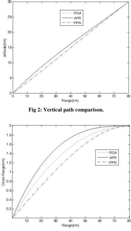
To demonstrate the effectiveness of this guidance law, it has been used in a 3DOF (point mass) simulation containing a standard atmosphere, and aerodynamic coefficients as functions of Mach number, angle of attack, and Reynolds number in tabulated form for RV model based on [46]. Results are shown in Figs.2-7 for a sample period of t=0.01s. It is understood that the optimum selection of B2 via RGA approach requires a very large computer resource. For this reason, the following approximate (near optimal) approach (APR) have been used. As first seen by Eisler and et al. [1] and can be seen in Fig. 2 by RGA approach, the optimal trajectory steers the RV to fly at higher altitudes as far as possible. This is equivalent to h2=g4, i.e. avc= amax and selection of 2 in such a manner that ahc=0 in the beginning of flight (For BTT it is equivalent to Lc=Lmax, and =180).

Table 1. Trajectory boundary conditions.

Initial Final

, km 80 0

, km 2 0

h, km 30 0

V, m s-1 4000 maximum

, deg 20 unconstrained

, deg 0 unconstrained

Also shown in these figures are the optimal trajectory (RGA) and the trajectory obtained from pure proportional navigation (PPN) with N=3 [47]. A fourth-order, fixed step, Runge-Kutta integrator is used in all simulations. The trajectory boundary conditions for the example problem are shown in Table 1. Figures 2 and 3 display the simulation flight path profiles. APR and RGA have the same vertical path, but slightly different horizontal paths, whereas PPN, which turns quickly to line up with the target. As just said, these first two simulations shift the majority of flight time to the higher altitudes, where drag is low. Therefore differences in horizontal paths and acceleration command (Fig. 4) have a very small effect on velocity profile (Fig. 7).

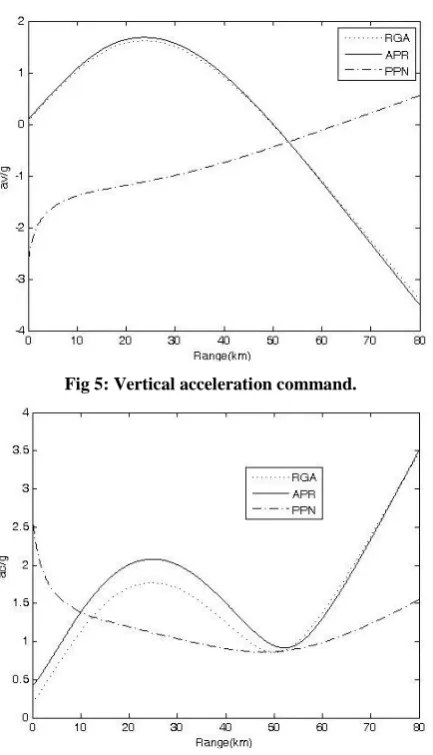
The acceleration command profiles shown in Figs. 4-6 reconfirm the turning rates between PPN and the other guidance schemes. The horizontal acceleration command profiles are shown in Fig. 4 and also show the increased turning rate applied by PPN to line up with the target. RGA initially chooses a middle ground between PPN and approximate scheme. Figures 5 and 6 display a good agreement in vertical and total acceleration command profiles for RGA and APR schemes.

Velocity-range profiles in Fig. 7 are grouped in a similar fashion to the flight profiles. Because of the altitude management in the APR and RGA guidance, the terminal velocities show small differences. The optimal velocity produced by RGA scheme is 1625 m s-1. The terminal velocity generated by APR method differs from it by about 0.3% (1620 m s-1), while the PPN solution is over 13% less (1410 m s-1). Note also that the times of flight for RGA and APR schemes are almost identical.

Uncertainties or off-nominal conditions in models characteristics have a profound effect on a guidance performance. The overall goal of guidance algorithm is the successful steering of the vehicle in spite of these

aerodynamics characteristics, and the atmospheric density. A Monte Carlo analysis was performed by introducing variations in vehicle aerodynamics (10%), atmospheric density (10%), and entry conditions (= h= 1000 m, = =1 deg, V= 10 m/s). Also the following wind profile was considered:

      

 

  

   



 





w2 w2

2

w2 w1

w1 w1

w2

w1 1 w2 2

w1 1

w1 w1

1

δ

) ( ) (

) δ ( ) δ (

) δ (

δ

h h V

V

h h h h h h

h

V V V V

V V

h h V

V Vw

where V1= 15 m/s, V2= 20 m/s, Vw1=Vw2= 5 m/s, hw1=10 km, hw2=20 km.

Finally, with a uniform distribution in uncertainties, 200 cases were conducted to assess the robustness of proposed guidance approach. The mean value and standard deviation resulted in the range were mR= -13.65 m and R= 4.24 m. These values were mC= -0.21 m and C= 0.32 m in the cross range. The scheme provides robust properties as indicated by results of Monte Carlo flight simulations. This robustness is the character of closed loop explicit guidance laws.

Fig 2: Vertical path comparison.

Fig 4: Horizontal acceleration command.

Fig 5: Vertical acceleration command.

Fig 6: Total acceleration command.

Fig 7: Velocity comparison.

5.

CONCLUDING REMARKS

A near optimal explicit guidance method was devised to obtain descent trajectories for a prescribed destination using differential flatness and inverse problem combination. The guidance commands are related to shape of trajectory, specified by a Bezier curve, to minimize the time spent in the denser parts of the atmosphere. During periods of command saturation, the instantaneous Bezier control points vary until sufficient control is available to follow the optimal trajectory. Optimal Bezier control points can be determined by using any parameter optimization method, such as Real-coded Genetic Algorithm (RGA), and implemented by an approximated logic (APR). The robustness of the algorithm in the face of worst case perturbations in the entry conditions, the aerodynamics characteristics, and the atmospheric density was examined by Monte Carlo simulation. The proposed method is characterized by the following advantages: 1) a priori satisfaction of the boundary conditions; 2) an absence of "wild" trajectories during path generation; 3) an analytical (parametric) representation of reference trajectory with minimum parameters; 4) applicability to any RV configuration, regardless of its lift-to-drag ratio or range of flight Mach number regime; 5) applicability to any control schemes (bank-to-turn or skid-to-turn), and 6) offline nominal trajectory and Time-to-Go independence. Comparison with the real coded genetic algorithm for the terminal velocity is excellent and far exceeds the pure proportional navigation solution.

6.

REFERENCES

[1] Eisler, G.R. and Hull, D.G. 1993. Guidance law for planar hypersonic descent to a point, J. of Guidance, Control, and Dynamics, V. 16, N. 2, 400-402.

[2] Eisler, G.R. and Hull, D.G. 1994. Guidance law for hypersonic descent to a point, Journal of Guidance, Control, and Dynamics, Vol. 17, No. 4, 649-54.

[3] Grälin, M.H., Telaar J., and Schottle U.M. 2004. Ascent and reentry guidance concept based on NLP-methods, Acta Astronautica, N. 55, 461-471.

[4] Shrivastava, S.K., Bhat, M.S., and Sinha, S.K. 1986. Closed-loop guidance of satellite launch vehicle- An overview, J. of the Institute of Engineers, N. 66, 62-76.

[6] Lu, P. 1993. Inverse dynamics approach to trajectory optimization for an aerospace plane. J. of Guidance, Control and Dynamics, V. 16, No. 4, 726-731.

[7] Borri, M., Bottasso, C.L., and Montelaghi, F. 1997. Numerical approach to flight dynamics. J. of Guidance, Control, and Dynamics, V. 20, No. 4, 742-747.

[8] Kato, O., Sugiura, I. 1986. An interpretation of airplane general motion and control as inverse problem. J. of Guidance, Control, and Dynamics, V. 9, No. 2, 198-204.

[9] Lane, S.H., and Stengel, R.S. 1988. Flight control design using non-linear inverse dynamics. Automatica, V. 24, 471-483.

[10]Sentoh, E., and Bryson, A.E. 1992. Inverse and optimal control for desired outputs. J. of Guidance, Control and Dynamics, V. 15, No. 3, 687-691.

[11]Hough, M.E. 1982. Explicit guidance along an optimal space curve. J. of Guidance, Control, and Dynamics, V. 12, No. 4, 495-504.

[12]Leng, G. 1998. Guidance algorithm design: a nonlinear inverse approach. J. of Guidance, Control, and Dynamics, V. 21, No. 5, 742-746.

[13]Lin, C.F., and Tsai, L.L. 1987. Analytical solution of optimal trajectory-shaping guidance. J. of Guidance, Control, and Dynamics, V. 10, No. 1, 61-66.

[14]Sinha, S.K., and Shrivastava, S.K., 1990. Optimal explicit guidance of multistage launch vehicle along three-dimensional trajectory. J. of Guidance, Control and Dynamics, V. 13, No. 3, 394-403.

[15]Taranenko, V.T., and Momdzhi, V.G. 1986. Direct Method of Modification in Flight Dynamic Problems, Moscow, Mashinostroenie Press (In Russian).

[16]Cameron, J.D.M. 1977. Explicit guidance equations for maneuvering re-entry vehicles. Proceedings of the IEEE Conference on Decision and Control, New York, USA: Inst. of Electrical and Electronics Engineers.

[17]Page, J., and Rogers, R. 1977. Guidance and control of maneuvering reentry vehicles. Proceedings of the IEEE Conference on Decision and Control, New York, USA: Inst. of Electrical and Electronics Engineers.

[18]Mortazavi, M. 2000. Trajectory Determination Using Inverse Dynamics and Reentry Trajectory Optimization, PhD thesis, Moscow Aviation Institute.

[19]Esmaelzadeh R., Naghash A., Mortazavi M. 2008. Explicit Reentry Guidance Law Using Bezier Curves. Transactions of the Japan Society for Aeronautical and Space Sciences, N. 170, 225-230.

[20]Naghash, A., Esmaelzadeh, R., Mortazavi, M., Jamilnia, R. 2008. Near Optimal Guidance Law for Descent to a Point Using Inverse Problem Approach. Aerospace Science and Technology, Vol. 12, No. 3, 241-247.

[21]Esmaelzadeh, R., Naghash, A., Mortazavi, M. 2008. Near optimal reentry guidance law using inverse problem approach. Journal of inverse problem in science and engineering, Vol. 16, No. 2, 187-198.

[22]Fliess M., L´evine J., Martin P., Rouchon P. 1995. Flatness and defect of nonlinear systems: introduction theory and examples. Int. Journal of Control, No. 61.

[23]Zerar M., Cazaurang F., Zolghadri A. 2005. LPV Modeling of Atmospheric Re-entry Demonstrator for Guidance Reentry Problem. Proceedings of the 44th IEEE Conference on Decision and Control, Spain.

[24]Morio V., Cazaurang F., Vernis P. 2009. Flatness-based hypersonic reentry guidance of a lifting-body vehicle. Control Engineering Practice, No. 17, 588-596.

[25]Sira-Ramirez H. 1999. Soft Landing on a Planet: A Trajectory Planning Approach for the Liouvillian Model. Proceedings of the American Control Conference, USA.

[26]Sun L.G.W., Zheng Z. 2009. Trajectory optimization for guided bombs based on differential flatness. Proceedings of the Chinese Control and Decision Conference.

[27]Neckel T., Talbot C., Petit N. 2003. Collocation and inversion for a reentry optimal control problem. Proceedings of the 5th International Conference on Launcher Tech.

[28]Archer, S.M., and Sworder, D.D. 1979. Selection of the guidance variable for a re-entry vehicle. J. of Guidance, Control and Dynamics, Vol. 2, No. 2, 130-138.

[29]Judd K.B., and McLain T.W. 2001. Spline based path planning for unmanned air vehicles. AIAA Guidance, Navigation, and Control Conf. & Exhibit, Canada.

[30]Shen Z. 2002. On-board three-dimensional constrained entry flight trajectory generation, PhD thesis, Iowa State University.

[31]Rogers, D.F., and Adams, J.A., 1990. Mathematical Elements for Computer Graphics, New York, McGraw-Hill, 1990.

[32]Nagatani K., Yosuke I., and Yutaka T. 2003. Sensor-based navigation for car-like mobile robots Sensor-based on a generalized Voronoi graph. Advanced Robotics, N. 17, 385-401.

[33]Zhang J., Raczkowsky J., Herp A. 1994. Emulation of spline curves and its applications in robot motion control. IEEE Conf. on Fuzzy Systems, Orlando, USA, 831-836.

[34]Myong H.S., Kyu J.L 2000. Bezier curve application in the shape optimization for transonic airfoils. the 18TH AIAA Applied Aerodynamics Conf., USA, 884-894.

[35]Venkataraman P. 1997. Unique solution for optimal airfoil design. the 15th AIAA Applied Aerodynamics Conf., USA, 205-215.

[36]Desideri J.A., Peigin S., and Timchenko S. 1999. Application of genetic algorithms to the solution of the space vehicle reentry trajectory optimization problem. INRIA Sophia Antipolice Research Report No. 3843.

[37]Rahman, T., Zhou H., Chen W. 2013. Bézier approximation based inverse dynamic guidance for entry glide trajectory. Control Conference (ASCC), 9th Asian.

[38]Betts, J.T. 1998. survey of numerical methods for trajectory optimization. Journal of Guidance, Control and Dynamics, Vol. 21, No. 2, 193-207.

Journal of Spacecraft and Rockets, Vol. 40, No. 6, 882-888.

[40]Yokoyama, N., Suzuki, S. 2005. Modified genetic algorithm for constrained trajectory optimization. J. of Guidance, Control and Dynamics, V. 28, No.1, 139-144.

[41]Deb, K. 2001. Multi-objective optimization using evolutionary algorithms, John-Wiley & Sons, Ltd., New York.

[42]Gen, M. and Cheng, R. 2000. Genetic algorithms & engineering optimization, John Wiley & Sons Inc., New York.

[43]Renders, J.M. and Flasse, S.P. 1996. Hybrid methods using genetic algorithms for global optimization. IEEE

Transactions on Systems, Man, and Cybernetics-Part B: Cybernetics, Vol. 26, No. 2, 243-258.

[44]Esmaelzadeh, R., Naghash, A. and Mortazavi, M. 2005. Hybrid trajectory optimization using genetic algorithms. Proceedings of the 1st International Conference on Modeling, Simulation and Applied Optimization, Sharjah, U.A.E.

[45]Lin, T.F., and et al. 2003. Novel approach for maneuvering reentry vehicle design. J. of Spacecraft and Rocket, V. 40, No. 5, 605-614.