Hydrol. Earth Syst. Sci., 19, 2491–2504, 2015 www.hydrol-earth-syst-sci.net/19/2491/2015/ doi:10.5194/hess-19-2491-2015
© Author(s) 2015. CC Attribution 3.0 License.
Using high-frequency water quality data to assess sampling
strategies for the EU Water Framework Directive
R. A. Skeffington1, S. J. Halliday1, A. J. Wade1, M. J. Bowes2, and M. Loewenthal3
1Dept. of Geography and Environmental Sciences, University of Reading, Reading, RG6 6DW, UK 2Centre for Ecology and Hydrology, Wallingford, Oxon., OX10 8BB, UK
3Environment Agency, Fobney Mead, Reading, RG2 0SF, UK
Correspondence to: R. A. Skeffington ([email protected])
Received: 17 December 2014 – Published in Hydrol. Earth Syst. Sci. Discuss.: 28 January 2015 Accepted: 8 May 2015 – Published: 26 May 2015
Abstract. The EU Water Framework Directive (WFD) re-quires that the ecological and chemical status of water bodies in Europe should be assessed, and action taken where possi-ble to ensure that at least “good” quality is attained in each case by 2015. This paper is concerned with the accuracy and precision with which chemical status in rivers can be mea-sured given certain sampling strategies, and how this can be improved. High-frequency (hourly) chemical data from four rivers in southern England were subsampled to simu-late different sampling strategies for four parameters used for WFD classification: dissolved phosphorus, dissolved oxy-gen, pH and water temperature. These data sub-sets were then used to calculate the WFD classification for each site. Monthly sampling was less precise than weekly sampling, but the effect on WFD classification depended on the close-ness of the range of concentrations to the class boundaries. In some cases, monthly sampling for a year could result in the same water body being assigned to three or four of the WFD classes with 95 % confidence, due to random sampling effects, whereas with weekly sampling this was one or two classes for the same cases. In the most extreme case, the same water body could have been assigned to any of the five WFD quality classes. Weekly sampling considerably reduces the uncertainties compared to monthly sampling. The width of the weekly sampled confidence intervals was about 33 % that of the monthly for P species and pH, about 50 % for dissolved oxygen, and about 67 % for water temperature. For water temperature, which is assessed as the 98th percentile in the UK, monthly sampling biases the mean downwards by about 1◦C compared to the true value, due to problems of assessing high percentiles with limited data. Low-frequency
measure-ments will generally be unsuitable for assessing standards ex-pressed as high percentiles. Confining sampling to the work-ing week compared to all 7 days made little difference, but a modest improvement in precision could be obtained by sam-pling at the same time of day within a 3 h time window, and this is recommended. For parameters with a strong diel vari-ation, such as dissolved oxygen, the value obtained, and thus possibly the WFD classification, can depend markedly on when in the cycle the sample was taken. Specifying this in the sampling regime would be a straightforward way to improve precision, but there needs to be agreement about how best to characterise risk in different types of river. These results sug-gest that in some cases it will be difficult to assign accurate WFD chemical classes or to detect likely trends using cur-rent sampling regimes, even for these largely groundwater-fed rivers. A more critical approach to sampling is needed to ensure that management actions are appropriate and sup-ported by data.
1 Introduction
each river basin and shall permit classification of water bod-ies into five classes. . . ” (EU, 2000, Annex V, Sect. 1.3). These classes are designated, in increasing order of quality, “bad”, “poor”, “moderate”, “good” and “high”. One specific aim of the directive is that all waters should be of at least “good” quality by the year 2015, though derogations from this are possible. If waters fail to meet this standard, then action must be taken to remedy the situation. Monitoring of waters and their assignment to quality classes is thus cen-tral to the operation of the WFD, though monitoring also has other objectives such as increasing system understand-ing and designunderstand-ing mitigation options. Because the quality of all waters varies both spatially and temporally, the represen-tativeness of water samples is a crucial issue. There is a large literature on the design of aquatic monitoring programmes, which invariably covers sampling problems. For instance, Hunt and Wilson (1986, Chap. 3) reviewed 386 references on water sampling up to 1986, Dixon and Chiswell (1996) found about 150 up to 1995, and more recently Strobl and Robil-lard (2008) and Horowitz (2013) have reviewed the subject further. There is general agreement in these references about the importance of defining specific objectives for monitoring. Here the WFD is reasonably specific, defining objectives for three types of monitoring, namely surveillance monitoring to establish the present status; operational monitoring aimed at those water bodies at risk of non-compliance with objectives, and investigative monitoring for establishing the reasons for non-compliance and the magnitude of accidental pollution episodes (EU, 2000, Annex V, Sect. 1.3). Both the former types have “assessment of change” as a sub-objective. More detailed guidance on sampling objectives is given in vari-ous guidance documents (e.g. EU, 2009). These are the re-sult of much discussion in expert committees, work groups, workshops, etc., but the diversity of surface waters in the EU means these can do little more than state the issues which should be taken into consideration, rather than giving spe-cific guidance.
The WFD also recognises that the variability of surface waters causes problems in classifying them and in trend de-tection. There is a trade-off between the improved precision and accuracy obtained by sampling more frequently and the increased costs incurred. The issue of sampling frequency is extensively discussed in the reviews quoted above. The WFD states “Frequencies shall be chosen so as to achieve an ac-ceptable level of confidence and precision” (EU, 2000 Annex V, Sect. 1.3.4). What is acceptable is left open, but estimates of confidence and precision have to be quoted in the River Basin Management Plans which are therefore open to pub-lic scrutiny. The WFD specifies that monitoring for physico-chemical determinands should be not less than 3 months, but leaves open the possibility that monitoring frequencies could be greater or smaller depending on expert judgement. The WFD also recognises the need to take seasonal varia-tion into account, but not, apparently, regular variavaria-tion on shorter timescales such as diurnal variation. This need is,
however, well recognised in the wider literature. Hunt and Wilson (1986, p. 52), for instance, state that where cyclic variations are of similar size to random variation, sampling
times “should be chosen so that representative sampling of
the cycle is achieved”.
The present paper uses high-frequency chemical data from four rivers in southern England to assess the accuracy and precision of the WFD classifications applied to them, and to evaluate some strategies for improving accuracy and preci-sion. The data were subsampled to simulate different sam-pling frequencies, and to simulate a variety of samsam-pling strategies. This approach has previously been used to eval-uate the influence of sampling strategy on stream concentra-tions (e.g. Kronvang and Bruhn, 1996; Bowes et al., 2009) and estimates of pollutant loading in rivers (e.g. Johnes, 2007; Cassidy and Jordan, 2011), but has not as far as we are aware been applied to WFD classifications. The paper also raises questions about the conclusions which can legiti-mately be drawn from current monitoring programmes.
2 Methods 2.1 Study sites
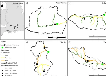
The catchments used for this study are shown in Fig. 1, and some relevant hydrological characteristics in Table 1. More detail on each site is given in the papers quoted in this sec-tion. All the rivers are affected to some extent by groundwa-ter abstractions and transfers, a common situation in southern England. The effects of these can be clearly seen in Table 1, with reduced specific flows in the Kennet and enhanced flows in The Cut due to water imports.
The upper River Kennet (Fig. 1a) was sampled at Milden-hall, some 2 km east of Marlborough (Palmer-Felgate et al., 2008). The catchment consists entirely of chalk of Creta-ceous age. The river is predominantly groundwater-fed, with a baseflow index of 0.94 (Table 1), hence a damped hy-drological response to rainfall. Land use is predominantly arable agriculture with some intensive livestock farming. The town of Marlborough (pop. ca. 8400) is the only signif-icant urban settlement. Above Marlborough sewage treat-ment works (STW), the Water Framework Directive classi-fication is “good”, deteriorating to “moderate” below (see http://maps.environment-agency.gov.uk/).
R. A. Skeffington et al.: Sampling strategies for the EU Water Framework Directive 2493
Figure 1. The four river catchments used in this study. The rivers are coloured according to their official status under the EU Water Framework
Directive (WFD), as calculated by the English Environment Agency (http://maps.environment-agency.gov.uk/). Larger towns are marked by initials: M, Marlborough; Ma, Maidenhead; B, Bracknell; A, Ascot; D, Dorchester.
Table 1. Some characteristics of the sampled rivers.
Catchment Precipitation ∗Mean Baseflow Population River area (km2) (mm yr−1) flow (m3s−1) index (2011 census)
Kennet 220 770 ca. 1.26 0.94 12 800
Enborne 148 790 1.31 0.53 18 300
The Cut 124 676 ca. 1.32 0.46 190 000
Frome 414 968 6.65 0.84 46 000
Data from the UK National River flow archive http://www.ceh.ac.uk/data/nrfa/index.html unless otherwise specified.∗Only the rivers Enborne and Frome are gauged at the sampling point. Flow in the Kennet was estimated
from gauging stations located approximately 2 km upstream. Flow in The Cut was estimated from a gauging station at Binfield (gauging 50 km2of the catchment), plus measured discharges from the sewage treatment works, plus an estimate of discharge from the lower part of the catchment based on that from the upper (Halliday et al., 2015).
The Cut (Fig. 1c) was sampled near its confluence with the River Thames at Bray (Wade et al., 2012; Halliday et al., 2015). The catchment geology is predominantly London Clay and Reading Beds (Palaeocene clays and sands), giving an impermeable catchment with a baseflow index of 0.46. The catchment population is around 190 000, mostly in the large urban centres of Bracknell and Maidenhead. Improved grassland covers 30 % of the catchment and 26 % is classed as arable, mostly in the northern half, and woodland occu-pies 15 %, mostly in the south. River flows are substantially increased by abstraction from the Thames for drinking wa-ter (Halliday et al., 2015) and its subsequent release through the STWs, increasing the specific runoff (Table 1). The WFD classification is mostly “poor”, being “moderate” only in the
upper reaches above the major conurbations. Note the river is called “The Cut”; hence “The” is capitalised throughout.
[image:3.612.136.458.404.483.2]2.2 High-frequency water sampling
Methods for collecting high-frequency water chemistry data varied somewhat between rivers: they are summarised here and are described in more detail in the papers cited be-low. Sampling of the River Enborne is described in Wade et al. (2012) and Halliday et al. (2014). Sampling began on 1 November 2009 and finished on 29 February 2012. Sam-pling frequency was hourly. A YSI 6600 multi-parameter sonde was used to measure a standard suite of parameters, including dissolved oxygen, pH and water temperature. A bankside mains-powered instrument, the Systea Micromac C, was used to make hourly measurements of total reactive phosphorus (TRP). The instrument uses the phosphomolyb-denum blue complexation method on an unfiltered sample, hence TRP is an operationally defined measurement, pre-dominantly comprised of orthophosphate (PO4)and readily hydrolysable P species.
The River Kennet at Mildenhall was sampled from Jan-uary 2004 to November 2006 and used the same instrumen-tal set-up as the Enborne, as described by Palmer-Felgate et al. (2008).
The Cut was sampled from April 2010 to February 2012 (Wade et al., 2012; Halliday et al., 2015). Sampling fre-quency was hourly and measurements of dissolved oxy-gen, pH and water temperature were made by a YSI multi-parameter sonde as above. Phosphorus species were mea-sured using a Hach Lange Phosphax Sigma which uses phosphomolybdenum blue complexation to measure TRP as above, and also total phosphorus (TP) by acid persulfate digestion after heating to 140◦C, at a pressure of 2.5 bar (359 kPa), followed by phosphomolybdenum blue complex-ation. There was no filtration step in either analysis.
The River Frome at East Stoke was sampled as described by Bowes et al. (2009) between 1 February 2005 and 31 Jan-uary 2006, as part of a much longer, lower-frequency study (Bowes et al., 2011). Samples of river water (500 mL) were taken from approximately the mid depth of the river using an automatic water sampler (Montec Epic, model 1011). Sam-pling frequency varied from two to four times per day during dry periods and up to eight samples per day during periods of rainfall. A total of 1358 samples were taken over the 1 year monitoring period. Total phosphorus was determined in the laboratory by digesting the sample with acidic potassium per-sulfate in an autoclave at 121◦C, then reacting with acidic ammonium molybdate reagent to produce phosphomolybde-num blue complex (Murphy and Riley, 1962). Soluble reac-tive phosphorus (SRP) was determined by filtering river wa-ter samples through a 0.45 µm cellulose nitrate membrane, and analysing for phosphate as above.
2.3 Statistical analysis
As the determination of the WFD status of a water is based on annual means, the data sets were divided into annual
sub-sets: 2010 and 2011 for the Enborne; 2004 and 2005 for the Kennet; 2011 for The Cut; and 2005 for the Frome. A stan-dard set of descriptive statistics was then calculated for all the data sets, including those required for WFD determina-tions in the UK, which are the mean for P and pH; the 10th percentile for dissolved oxygen; and the 98th percentile for water temperature. The analysis in this paper is restricted to these four variables. Each of the high-frequency annual data sets was then resampled using two different sampling fre-quencies and five different sampling strategies, to create a series of ten sampling scenarios. Sampling frequency was ei-ther monthly or weekly. Within each of these, the strategies were (with abbreviations in brackets) the following:
– sampling at any time (ANY);
– sampling on any day of the week, but restricted to normal working hours, defined as between 09:00 and 17:59 UTC (AW9-18);
– sampling on Monday to Friday only, and also restricted to normal working hours (MF9-18). This is the com-monest sampling approach used by the regulatory agen-cies;
– sample collection on any day, but restricted to a 3 h win-dow between 09:00 and 11:59 UTC (AW9-12); – sample collection restricted to Monday to Friday and
also restricted to a 3 h window between 09:00 and 11:59 UTC (MF9-12).
Each of these re-sampling strategies was applied to each data set using the MATLAB function datasample (Mathworks, 2014). This was set up to sample at random from the appro-priate hourly time series using a uniform distribution. Only one sample was taken from a given month or week, to repli-cate a real sampling programme. The data sets were resam-pled 1000 times, each generating a secondary data set which represents a set of samples which might have been collected if the given sampling strategy had been implemented. There are thus 1000 implementations of each sampling strategy, which were used to generate statistics showing the resulting distributions of measurements and the WFD classifications which would have been obtained. In particular, the means and 95 % confidence limits on the means were calculated and are used in the following analysis. The 95 % confidence limits were calculated as the 2.5th and 97.5th percentiles of the dis-tribution of means generated by the 1000 trials – this is the percentile bootstrap confidence interval (Davison and Hink-ley, 1997; Sect. 5.3), which will simply be referred to in this paper as the confidence interval (CI).
3 Results and discussion
R. A. Skeffington et al.: Sampling strategies for the EU Water Framework Directive 2495
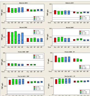
Figure 2. Means and 95 % confidence intervals for phosphorus species generated by resampling from high-frequency data. First five columns:
monthly sampling; remaining five: weekly sampling. Red bars – at any date or time; green – working hours (09:00–17:59) only; blue – 09:00–11:59 only. AW – on any day of the week; MF – Monday to Friday only. Horizontal lines represent Water Framework Directive class boundaries where applicable, from the bottom: High/Good; Good/Moderate; Moderate/Poor. Note the different scale for The Cut. P species are defined in Sect. 2.2: TRP – total reactive phosphorus; SRP – soluble reactive phosphorus; TP – total phosphorus.
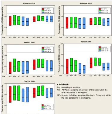
water temperature – given different sampling strategies. The five bars on the left of each graph represent monthly sam-pling; those on the right, weekly sampling. Within each of these the sampling strategies represent (from left to right) the ANY; AW9-18; MF9-18; AW9-12; and MF9-12 sampling strategies (see previous paragraph). The boundaries between different river quality classes in the UK implementation of the WFD are also shown where appropriate. The statistics plotted are those used in the UK for the WFD: means for pH and P species; the 10th percentile for dissolved oxygen; and the 98th percentile for water temperature.
3.1 Monthly versus weekly sampling
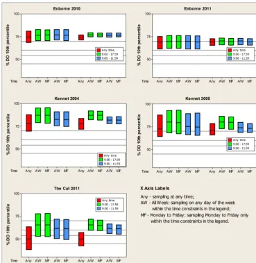
Figure 3. Mean 10th percentiles and 95 % confidence intervals for dissolved oxygen generated by resampling from high-frequency data. First
five columns: monthly sampling; remaining five: weekly sampling. Horizontal lines represent Water Framework Directive class boundaries – from the top: High/Good; Good/Moderate; Moderate/Poor; Poor/Bad.
contained entirely within the moderate class. Similarly, the 95 % CI for MF9-18 sampling of TRP on The Cut covers 247 µg P L−1(480–727), whereas the corresponding 95 % CI for weekly sampling is only 70 µg P L−1(546–616), though all samples are in the “poor” WFD class. The width of the weekly sampled confidence intervals was about 33 % that of the monthly for P species and pH (Figs. 2 and 4), about 50 % for dissolved oxygen (Fig. 3) and about 67 % for temperature (Fig. 5). Whether the improvement of precision of weekly sampling makes any difference to the possible range of WFD classes depends on the closeness of the range of concentra-tions to the class boundaries. For instance, monthly sampling of temperature is less precise than weekly (Fig. 5), but this makes no difference to the WFD classification except on The Cut, whereas for P species (Fig. 2) the difference is consid-erable.
R. A. Skeffington et al.: Sampling strategies for the EU Water Framework Directive 2497
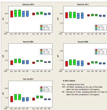
Figure 4. Means and 95 % confidence intervals for pH generated by resampling from high-frequency data. First five columns: monthly
sampling; remaining five: weekly sampling. The WFD class is uniformly “high” (pH>6.60).
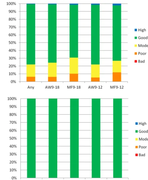
sampling and 89 % for weekly sampling (Fig. 6). Assuming DO concentrations stayed the same for 5 years, the probabil-ity of the classification being correct in every year is only 4 % (0.525)with monthly sampling, whereas it is 54 % (0.895)
with weekly sampling. The potential for generating spuri-ous “trends” in the WFD classification due to purely random sampling effects is obvious, if the sampling frequency is not great enough. For TRP on the Kennet (Fig. 7), weekly sam-pling always produces the correct classification of “good”, whereas with monthly sampling the classification is cor-rect only 65–75 % of the time. Proportions of other clas-sifications are “moderate”, 16–20 %; “poor”, 5–11 %; and “high”, 0–2 %, indicating the considerable uncertainty and wide range of possible classifications if the sampling fre-quency is not high enough. These considerations apply when the confidence intervals of the mean re-sampled concentra-tions crosses one or more WFD class boundaries – inspec-tion of Figs. 2–5 shows where this occurs. For some cases,
e.g. pH (Fig. 4), class boundaries are not crossed and any sampling strategy always gives the same classification.
Figure 5. Mean 98th percentiles and 95 % confidence intervals for water temperature generated by resampling from high-frequency data.
First five columns: monthly sampling; remaining five: weekly sampling. Horizontal line represents the Water Framework Directive class boundary between “high” (<20◦C) and “good”.
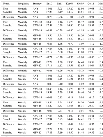
and sampling strategy, “true” being defined as the temper-ature calculated from all the measured data for the particu-lar frequency, strategy and river. Table 2 shows that monthly sampling is underestimating water temperatures by about 1◦C, sometimes more, whereas weekly sampling overesti-mates less consistently, by about 0.1◦C. These differences arise from the methods used to interpolate the 98th percentile temperature. When there are not many measurements (as in the monthly samples here), a systematic bias is likely as well as wide confidence intervals. The problems involved in the estimation of percentiles used as water quality standards are extensively discussed by Ellis and Lacey (1980), who note that the confidence limits are likely to be very wide for high (or low) percentiles and depend markedly on the underly-ing distributions of the measured values. The adoption of a 98th percentile as a standard was probably intended to apply to continuously measured temperature data where the large
number of data points reduces both random error and sys-tematic bias in estimation of the percentile. Use of a high percentile as a standard with spot measurements, which are typically fewer in number, needs to be more critically evalu-ated.
3.2 Diurnal sampling precision
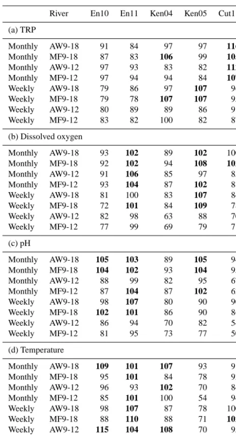
One aim of this paper is to investigate whether restricting the times at which samples are taken would improve the precision of the estimates for the chemical variables. This can be measured by comparing the height of each bar in Figs. 2–5 with the bar corresponding to unrestricted sam-pling (“ANY”). Table 3 shows a quantitative measure of this, i.e. 95 % CI(s)/95 % CI(Any)expressed as a percentage, where
95 % CI(s) is the 95 % confidence interval for a particular
strategy and 95 % CI(Any) is the 95 % CI for sampling at
R. A. Skeffington et al.: Sampling strategies for the EU Water Framework Directive 2499
Table 2. Sampled and true 98th percentile temperatures for the rivers and sampling strategies.
Temp. Frequency Strategy En10 En11 Ken04 Ken05 Cut11 Mean
True Monthly ANY 18.01 17.05 15.20 15.80 19.08 17.03 Sampled Monthly ANY 17.28 16.19 14.19 14.51 18.17 16.07
Difference Monthly ANY −0.73 −0.86 −1.01 −1.29 −0.91 −0.96
True Monthly AW9-18 18.40 17.16 15.70 16.32 20.01 17.52 Sampled Monthly AW9-18 17.59 16.38 14.90 15.14 18.97 16.59
Difference Monthly AW9-18 −0.81 −0.78 −0.80 −1.18 −1.04 −0.92
True Monthly MF9-18 18.36 17.74 15.50 16.30 20.01 17.58 Sampled Monthly MF9-18 17.53 16.38 14.80 15.21 18.89 16.56
Difference Monthly MF9-18 −0.83 −1.36 −0.70 −1.09 −1.12 −1.02
True Monthly AW9-12 17.88 16.86 14.00 14.40 18.81 16.39 Sampled Monthly AW9-12 17.17 16.08 13.67 13.60 17.98 15.70
Difference Monthly AW9-12 −0.71 −0.78 −0.33 −0.80 −0.83 −0.69
True Monthly MF9-12 17.79 17.38 13.90 14.40 18.98 16.49 Sampled Monthly MF9-12 17.14 16.12 13.54 13.65 18.04 15.70
Difference Monthly MF9-12 −0.65 −1.26 −0.36 −0.75 −0.94 −0.79
True Weekly ANY 18.01 17.05 15.20 15.80 19.08 17.03
Sampled Weekly ANY 18.01 17.15 15.24 15.82 19.42 17.13
Difference Weekly ANY 0.00 0.10 0.04 0.02 0.34 0.10
True Weekly AW9-18 18.40 17.16 15.70 16.32 20.01 17.52 Sampled Weekly AW9-18 18.39 17.29 15.84 16.40 20.16 17.62
Difference Weekly AW9-18 −0.01 0.13 0.14 0.08 0.15 0.10
True Weekly MF9-18 18.36 17.74 15.50 16.30 20.01 17.58 Sampled Weekly MF9-18 18.29 17.43 15.63 16.31 20.30 17.59
Difference Weekly MF9-18 −0.07 −0.31 0.13 0.01 0.29 0.01
True Weekly AW9-12 17.88 16.86 14.00 14.40 18.81 16.39 Sampled Weekly AW9-12 17.94 16.95 14.49 14.41 19.13 16.58
Difference Weekly AW9-12 0.06 0.09 0.49 0.01 0.32 0.19
True Weekly MF9-12 17.79 17.38 13.90 14.40 18.98 16.49 Sampled Weekly MF9-12 17.85 17.19 14.30 14.44 19.32 16.62
Difference Weekly MF9-12 0.06 −0.19 0.40 0.04 0.34 0.13
Temperatures in◦C. Abbreviations for the rivers are, respectively (Enborne, 2010, 2011; Kennet, 2004, 2005), The Cut 2011.
Strategy abbreviations: AW9-18, all week, working hours (09:00 to 17:59); MF9-18, Monday to Friday, working hours; AW9-12, all week, 09:00 to 11:59; and MF9-12, Monday to Friday, 09:00 to 11:59. The final column is the mean across all the rivers.
precision of the estimates in 71 % of cases – those where it does not do so are highlighted in the table. The most con-sistent improvements in precision are obtained using the 3 h sampling strategies (AW9-12 and MF9-12) for TRP, DO and pH with weekly sampling. Monthly sampling shows a sim-ilar pattern but is less consistent. In general, the 3 h strate-gies improve the precision more than the full working hours strategies (AW9-18 and MF9-18) – the average CI is 88 % of unrestricted for the 9–12 strategies versus 95 % for the
Figure 6. The probability that sampling dissolved oxygen on The
Cut for 1 year would put the river into a given WFD class,
(a) monthly sampling, and (b) weekly sampling. Strategy labels:
Any – at any time; AW9-18 – all week, working hours (09:00 to 17:59); MF9-18 – Monday to Friday, working hours; AW9-12 – all week, 09:00 to 11:59; MF9-12 – Monday to Friday, 09:00 to 11:59.
four chemical variables, and thus a more accurate estimate of the WFD class.
3.3 Different sampling strategies lead to different estimates of variables
It is clear from Figs. 2 to 5 that different sampling strategies give different estimates for the variables being considered. Apart from the differences in water temperature between monthly and weekly sampling referred to in Sect. 3.1, these are largely due to diel variations in processes affecting the variables. It is well known that DO has a strong diel variation due to the balance between photosynthesis and respiration, with low DO concentrations at night when there is no photo-synthesis and high concentrations during the day when pho-tosynthesis is active. This explains the patterns seen in Fig. 3, when the AW/MF9-18 strategies have higher DO concentra-tions than the average for the entire 24 h (ANY), and the AW/MF9-12 strategies are intermediate (as DO concentra-tions are generally higher in the afternoon). The patterns are most pronounced on The Cut, which has a very strong diel DO cycle (Wade et al., 2012; Halliday et al., 2015), and least on the Enborne, where heavy riparian shading due to
decid-Figure 7. The probability that sampling TRP on the River Kennet
for 1 year would put the river into a given WFD class, (a) monthly sampling, and (b) weekly sampling. Strategy labels: Any – at any time; AW9-18, all week, working hours (09:00 to 17:59); MF9-18, Monday to Friday, working hours; AW9-12, all week, 09:00 to 11:59; and MF9-12, Monday to Friday, 09:00 to 11:59.
uous trees restricts a strong diel DO cycle to the early spring (Halliday et al., 2014). The same cycle can be seen in the pH values (Fig. 4), where higher pH in the AW/MF9-18 samples is due to lower carbonic acid concentrations during the day because of photosynthetic uptake of carbon. Likewise, the prevalence of high water temperatures is lower in the morn-ing than for the whole day, or even the full 24 h (Fig. 5). Phos-phorus species have a less obvious pattern (Fig. 2), though there is a suggestion that MF values are slightly higher than AW values, reflecting a different outflow pattern from sewage treatment works between weekday and weekend (see Halli-day et al., 2014).
[image:10.612.309.547.66.356.2]R. A. Skeffington et al.: Sampling strategies for the EU Water Framework Directive 2501
Table 3. 95 % confidence intervals for each strategy as a percentage
of the 95 % CI for sampling at any time.
River En10 En11 Ken04 Ken05 Cut11
(a) TRP
Monthly AW9-18 91 84 97 97 116
Monthly MF9-18 87 83 106 99 105
Monthly AW9-12 97 93 83 82 112
Monthly MF9-12 97 94 94 84 107
Weekly AW9-18 79 86 97 107 96
Weekly MF9-18 79 78 107 107 95
Weekly AW9-12 80 89 89 86 91
Weekly MF9-12 83 82 100 82 87
(b) Dissolved oxygen
Monthly AW9-18 93 102 89 102 100
Monthly MF9-18 92 102 94 108 102
Monthly AW9-12 91 106 85 97 85
Monthly MF9-12 93 104 87 102 88
Weekly AW9-18 81 100 83 107 84
Weekly MF9-18 72 101 84 109 78
Weekly AW9-12 82 98 63 88 70
Weekly MF9-12 77 99 69 79 71
(c) pH
Monthly AW9-18 105 103 89 105 94
Monthly MF9-18 104 102 93 104 95
Monthly AW9-12 88 99 82 95 67
Monthly MF9-12 87 104 87 102 63
Weekly AW9-18 98 107 80 90 90
Weekly MF9-18 102 101 86 90 86
Weekly AW9-12 86 94 70 82 54
Weekly MF9-12 81 95 73 77 50
(d) Temperature
Monthly AW9-18 109 101 107 93 91
Monthly MF9-18 95 101 84 78 93
Monthly AW9-12 96 93 102 70 84
Monthly MF9-12 85 101 100 54 94
Weekly AW9-18 98 107 87 78 100
Weekly MF9-18 88 110 88 71 102
Weekly AW9-12 115 104 108 70 95
Weekly MF9-12 117 110 108 69 92
Abbreviations for the rivers are, respectively (Enborne, 2010, 2011; Kennet, 2004, 2005), The Cut 2011; AW9-18, all week, working hours (09:00 to 17:59); MF9-18, Monday to Friday, working hours; AW9-12, all week, 09:00 to 11:59; and MF9-12, Monday to Friday, 09:00 to 11:59. Percentages greater than 100 are highlighted in bold font.
throughout the 24 h period, including low DO concentrations during the night. Conversely it could be argued that since the boundaries between the WFD classes are derived in the UK from statistical associations between chemical parame-ters and biological quality based on sampling at conventional times, i.e. during working hours, then the correct classifica-tion is “good”. Whether “good” is a reasonable representa-tion may depend on the diel dynamics of DO at the particu-lar site. The Cut is a productive stream with both high photo-synthesis and respiration rates – DO concentrations can fall to as little as 27 % at night (Wade et al., 2012; Halliday et al., 2015). The Enborne in 2011 would also have been
classi-fied as “good”, but the magnitude of diel fluctuations is much smaller, with night-time DO concentrations no lower than 60 % (Halliday et al., 2014). Clearly The Cut is much more at risk of deleterious effects due to anoxia than the Enborne, but the daytime sampling regime does not register this dif-ference very strongly (Fig. 3). If the issue is low night-time DO concentrations, and the measurements are available be-cause the site is being continuously monitored, then it would seem more logical to use measurements made at night as the standard. The Cut might however be seen as an extreme case given its high STW load, and comparing the working day and anytime means and CIs in Fig. 3 shows that working day sampling is a better representation of the full range of DO concentrations on the Enborne than The Cut, with the Ken-net intermediate. Based on this sample of three rivers, it may be that daytime sampling for DO is not a good measure of risk for rivers with high respiration rates due to organic load-ing and/or high rates of primary production. This would need further investigation on more sites. What is not satisfactory, however, is that it is possible to obtain such widely differ-ing WFD classifications because the sampldiffer-ing time is not de-fined. Defining a sampling time as part of the assessment pro-cedure would be a straightforward process and reduce some of the uncertainty being discussed here, as previously sug-gested for The Cut by Halliday et al. (2015).
3.4 Differences between years
the greater variation in most concentrations in 2010 observ-able in Figs. 2–5. In general, the range in concentrations is determined by individual flow events which are not appar-ent in annually aggregated statistics, but this study illustrates that such differences do occur and will add to the variation observed.
4 Wider discussion
This study shows that for these four rivers, the WFD class cannot be assigned with 95 % confidence for a number of variables and sampling strategies. Taking the strategy most commonly used in practice, MF9-18, the WFD class cannot be assigned for monthly sampling of phosphorus on the En-borne in 2010 and 2011 and the Kennet in 2004; dissolved oxygen on the Enborne in 2011, the Kennet in 2005 and The Cut in 2011; and water temperature on The Cut in 2011. For weekly sampling, the WFD class cannot be assigned for dis-solved oxygen on the Enborne in 2011 and The Cut in 2011, and temperature on The Cut in 2011. Clearly, weekly sam-pling generates less ambiguity, and this matches the conclu-sions of Johnes (2007) that monthly sampling gave highly uncertain load estimates for a variety of British rivers, in-cluding the Enborne. In contrast, the WFD class can be as-signed unambiguously for pH on all rivers and temperature in most (all “high”) and phosphorus on The Cut (“poor”), whatever the sampling strategy. Where the sample mean is close to a class boundary (as for dissolved oxygen on the Enborne 2010), then consistent assignment to a single class is unlikely, but this should not be a major issue as long as the potential size of the confidence intervals is realised when drawing conclusions. Of most concern are situations where the confidence interval crosses several classes, as with dis-solved oxygen on The Cut, which can be assigned to four WFD classes with 95 % confidence given monthly sampling, as opposed to two or three classes with weekly sampling. It seems clear that if the aim is to identify WFD classes it would be better to spend limited resources on monitoring dissolved oxygen than pH in these rivers. This sort of judgement should be made in the light of technical knowledge and considering the objectives of the monitoring programme. For instance, all these rivers are fed by well-buffered calcareous groundwater and monitoring shows the pH to be well above the high/good boundary. A change of WFD status for pH is thus unlikely and occasional monitoring (e.g. twice a year) would suffice. The same considerations might apply to P concentrations on The Cut, which are unlikely to drop below “poor” in view of the high P load from sewage treatment works, except that here the WFD objectives specify that P concentrations should be reduced in an attempt to improve the classification. Hence more frequent monitoring is justified even though the clas-sification is likely to remain “poor” for the foreseeable fu-ture, and it becomes relevant that the 95 % confidence inter-val for monthly sampling is around 250 µg P L−1as opposed
to 70 µg P L−1for weekly sampling. For detection of likely trends, weekly sampling will be required. This differentiated approach to monitoring is suggested in the WFD. In practice, sampling effort may not be affected much if more frequent samples have to be taken from the same site in any case, but analytical effort may be reduced given that different determi-nands are analysed using different equipment.
The results show that there is little difference between sampling Monday to Friday or during the whole week. Dif-ferences can be seen in Figs. 2–5, but they are generally small in magnitude and not consistent in direction. Phosphorus is the determinand for which differences might be most likely, as the pattern of sewage treatment works output differs some-what between weekdays and weekends (e.g. Halliday et al., 2014), but this is not apparent in Fig. 2. On the other hand, re-stricting sampling to the 3 h period between 09:00 and 11:59 leads to an improvement in precision for TRP, dissolved oxy-gen and pH, especially with weekly sampling (Table 3). The improvement is modest, amounting to a narrowing of the 95 % confidence interval by about 13 % for P, 20 % for dis-solved oxygen and 25 % for pH, for weekly samples, but it is consistent. For monthly samples the corresponding figures are 6, 6 and 12 % respectively, and the changes are not com-pletely consistent in direction. For 98th percentile water tem-perature, there is no improvement in precision from restrict-ing samplrestrict-ing times. The biggest improvements are shown by the determinands with the strongest diel variation (pH and dissolved oxygen), but are apparent for P as well. These im-provements in precision seem worthwhile, so restricting the sampling time to a 3 h window seems a useful strategy, as it would be easy and cheap to implement.
haz-R. A. Skeffington et al.: Sampling strategies for the EU Water Framework Directive 2503 ards in this area”. The conclusion for estimating the WFD
limits is that the 98th percentile criterion should only be used where there are sufficient values to calculate a percentile, and cannot be done with spot sampled values at frequencies of weekly or greater.
One of the implications of the results in this paper is that the precision of sampling needs to be taken into account when designing mitigation strategies or other management interventions. For instance, managers should be discouraged from basing mitigation plans on non-compliance of one loca-tion in one year, in circumstances when the non-compliance could simply be due to sampling error. This will require a critical case-by-case look at each location and sampling strat-egy.
This study has also shown the need to define more pre-cisely what a sample taken for WFD monitoring is meant to represent. Different WFD classifications can be obtained by regular sampling at different times of day, especially for variables with a strong diel variation, such as dissolved oxy-gen. This is surely an unsatisfactory situation, and it would be better to define a relatively narrow sampling time range to standardise this. There also needs to be some debate about whether a daytime sample for dissolved oxygen adequately represents the risk of anoxia occurring in all types of river, given the variety of behaviour exhibited by the Enborne and The Cut. Similar considerations apply to seasonal sampling, though are not covered in this paper. For instance, Rozemei-jer et al. (2014) criticised the use of summer-only sampling for assessing nutrient losses from agriculture to surface water and groundwater.
This study is based on an illustrative but restricted sam-ple of four rivers, and so must be applied with caution else-where. For instance, in the international context, these rivers are rather small (Table 1), though typical of rivers to which the WFD is applied in the UK. The conclusions may not be appropriate for much larger rivers – for instance, Liu et al. (2014) used an objective method to optimise sampling frequencies on the Xiangjiang River in China, concluding that adequate characterisation could be obtained by sam-pling at intervals varying between every 2 months and every 6 months. The Xiangjiang River, however, is a major tribu-tary of the Yangtze, draining an area of 85 000 km2, and sam-pling less frequently than once a month may be appropriate here as larger rivers will tend to have slower responses. Nad-deo et al. (2013) suggested that for some rivers in southern Italy, of about the size of the Frome in this study or slightly larger, sampling frequencies could be reduced in some cases to less than once a month without affecting the WFD clas-sification. However, neither of these studies considered sam-pling frequencies greater than monthly, assuming implicitly that monthly sampling gives the “correct” value. As shown in the present paper for these English rivers, this is not necessar-ily the case: a conclusion also supported in the context of load estimation by the work of Johnes (2007). The other relevant characteristic of the four rivers in the present study is their
high baseflow index. This will reduce the temporal variabil-ity of most variables and hence increase sampling precision for a given sampling frequency. If the present methodology was applied to flashier rivers such as those studied by Cas-sidy and Jordan (2011), the confidence limits observed would probably be even wider.
5 Conclusions
Overall, a more critical attitude needs to be taken towards wa-ter sampling in support of the WFD in rivers such as these. For many parameters, routine monthly sampling is unlikely to be able to assign a classification accurately or to detect trends unless they are very large. However, for some param-eters, such as pH in this case, monthly sampling is unneces-sarily frequent and possibly a waste of resources. The wide confidence intervals observed even for weekly sampling in some cases imply that there is a real possibility of identify-ing deleterious “trends” which do not really exist and wast-ing resources trywast-ing to correct them, or alternatively failwast-ing to identify genuine water quality reductions and thus not tak-ing the necessary improvement actions. This is particularly so given differences between years which are most proba-bly driven by varying hydrological conditions. The precision and accuracy of measurements can be improved by specify-ing a samplspecify-ing time interval, but a realistic assessment of the uncertainty attached to any given WFD classification seems essential before taking management action.
Acknowledgements. We would like to thank the Natural
Environ-ment Research Council for funding the monitoring of the rivers Frome and Kennet; the Engineering and Physical Sciences Re-search Council for funding the LIMPIDS project (EP/G019967/1) as part of which the Enborne and The Cut were monitored; and L. Palmer-Felgate, E. Gozzard, J. Newman, C. Roberts, L. Armstrong, S. Harman, and H. Wickham for providing the field and laboratory support that produced the Kennet, Cut and Enborne data sets.
Edited by: B. Kronvang
References
Bowes, M. J., Leach, D. V., and House, W. A.: Seasonal nutrient dy-namics in a chalk stream: the River Frome, Dorset, UK, Sci. To-tal Environ., 336, 225–241, doi:10.1016/j.scitotenv.2004.05.026, 2005.
Bowes, M. J., Smith, J. T., and Neal, C.: The value of high-resolution nutrient monitoring: A case study of the River Frome, Dorset, UK, J. Hydrol., 378, 82–96, doi:10.1016/j.jhydrol.2009.09.015, 2009.
of the River Frome (UK) from 1965 to 2009: Is phosphorus mit-igation finally working?, Sci. Total Environ., 409, 3418–3430, doi:10.1016/j.scitotenv.2011.04.049, 2011.
Cassidy, R. and Jordan, P.: Limitations of instantaneous water qual-ity sampling in surface-water catchments: comparison with near-continuous phosphorus time-series data, J. Hydrol., 405, 182– 193, 2011.
Davison, A. C. and Hinkley, D. V.: Bootstrap Methods and their Applications, Cambridge Series in Statistical and Probabilistic Mathematics, Cambridge University Press Cambridge, 1997. Dixon, W. and Chiswell, B.: Review of aquatic monitoring
pro-gram design, Water Res., 30, 1935–1948, doi:10.1016/0043-1354(96)00087-5, 1996.
Ellis, M. A. and Lacey, R. F.: Sampling; defining the task and plan-ning the scheme, Water Pollut. Control., 79, 452–467, 1980. EU: Directive 2000/60/EC of the European Parliament and of the
Council of 23 October 2000 establishing a framework for Com-munity action in the field of water policy, Official Journal of the European Communities, L327, 1–70, 2000.
EU: Common implementation strategy for the Water Framework Directive (2000/60/EC). Guidance document No. 19: guidance on surface water chemical monitoring under the Water Frame-work Directive, Luxembourg Technical Report 2009-025, 2009. Halliday, S. J., Skeffington, R. A., Bowes, M. J., Gozzard, E.,
New-man, J. R., Loewenthal, M., Palmer-Felgate, E. J., Jarvie, H. P., and Wade, A. J.: The water quality of the River Enborne, UK: observations from high-frequency monitoring in a rural, lowland river system, Water, 6, 150–180, 2014.
Halliday, S. J., Skeffington, R. A., Wade, A. J., Bowes, M. J., Goz-zard, E., Newman, J. R., Loewenthal, M., Palmer-Felgate, E. J., and Jarvie, H. P.: High-frequency water quality monitoring in an urban catchment: hydrochemical dynamics, primary production and implications for the Water Framework Directive, Hydrol. Process., doi:10.1002/hyp.10453, in press, 2015.
Horowitz, A. J.: A review of selected inorganic surface water quality-monitoring practices: are we really measuring what we think, and if so, are we doing it right?, Environ. Sci. Technol., 47, 2471–2486, 2013.
Hunt, D. T. E. and Wilson, A. L.: The chemical analysis of water: general principles and techniques, 2nd Edn., Royal Society of Chemistry, London, 1986.
Johnes, P.: Uncertainties in annual riverine phosphorus load esti-mation: impact of load estimation methodology, sampling fre-quency, baseflow index and catchment population density, J. Hy-drol., 332, 241–258, 2007.
Kronvang, B. and Bruhn, A.: Choice of sampling strategy and es-timation method for calculating nitrogen and phosphorus trans-port in small lowland streams, Hydrol. Process., 10, 1483–1501, 1996.
Liu, Y., Zheng, B., Wang, M., Xu, Y., and Qin, Y.: Optimization of sampling frequency for routine river water quality monitoring, Sci. China Chem., 57, 772–778, 2014.
MATLAB: available at: http://www.mathworks.co.uk/products/ matlab/, last access: 20 September 2014.
Murphy, J. and Riley, J.: A modified single solution method for the determination of phosphate in natural waters, Anal. Chim. Acta, 27, 31–36, 1962.
Naddeo, V., Scannapieco, D., Zarra, T., and Belgiorno, V.: River wa-ter quality assessment: Implementation of non-parametric tests for sampling frequency optimization, Land Use Pol., 30, 197– 205, 2013.
Palmer-Felgate, E. J., Jarvie, H. P., Williams, R. J., Mortimer, R. J. G., Loewenthal, M., and Neal, C.: Phosphorus dynamics and pro-ductivity in a sewage-impacted lowland chalk stream, J. Hydrol., 351, 87–97, doi:10.1016/j.jhydrol.2007.11.036, 2008.
Rozemeijer, J. C., Klein, J., Broers, H. P., van Tol-Leenders, T. P., and van der Grift, B.: Water quality status and trends in agriculture-dominated headwaters; a national monitoring net-work for assessing the effectiveness of national and European manure legislation in The Netherlands, Environ. Monitor. As-sess., 186, 8981–8995, 2014.
Strobl, R. O. and Robillard, P. D.: Network design for water quality monitoring of surface freshwaters: A review, J. Environ. Man-age., 87, 639–648, doi:10.1016/j.jenvman.2007.03.001, 2008. UK National River Flow Archive: available at: http://www.ceh.ac.
uk/data/nrfa/index.html, last access: 14 September 2014. Wade, A. J., Palmer-Felgate, E. J., Halliday, S. J., Skeffington,